Optimal Operation and Market Integration of a Hybrid Farm with Green Hydrogen and Energy Storage: A Stochastic Approach Considering Wind and Electricity Price Uncertainties

Abstract

In recent years, growing interest has emerged in investigating the integration of energy storage and green hydrogen production systems with renewable energy generators. These integrated systems address uncertainties related to renewable resource availability and electricity prices, mitigating profit loss caused by forecasting errors. This paper focuses on the operation of a hybrid farm (HF), combining an alkaline electrolyzer (AEL) and a battery energy storage system (BESS) with a wind turbine to form a comprehensive HF. The HF operates in both hydrogen and day-ahead electricity markets. A linear mathematical model is proposed to optimize energy management, considering electrolyzer operation at partial loads and accounting for degradation costs while maintaining a straightforward formulation for power system optimization. Day-ahead market scheduling and real-time operation are formulated as a progressive mixed-integer linear program (MILP), extended to address uncertainties in wind speed and electricity prices through a two-stage stochastic optimization model. A bootstrap sampling strategy is introduced to enhance the stochastic model’s performance using the same sampled data. Results demonstrate how the strategies outperform traditional Monte Carlo and deterministic approaches in handling uncertainties, increasing profits up to 4% per year. Additionally, a simulation framework has been developed for validating this approach and conducting different case studies.

1. Introduction

The integration of renewable energy sources in electrical systems has increased significantly in recent years [1]. Nonetheless, the intermittent availability of these sources presents challenges in terms of grid stability. A potential solution to this issue is the use of energy storage systems (ESSs) [2]. Lithium batteries are the most promising ESS technology due to their energy density and reduced costs [3].

Another possibility to consider is to utilize electricity for green hydrogen production [4]. This can be achieved by means of an electrolyzer, which uses electrical energy to produce hydrogen by splitting water molecules. Alkaline electrolyzers (AELs) are considered to be the most mature technology within their field [5].

These devices conform a system that can participate in both electricity and hydrogen markets. Modeling techniques should accurately address the components of such a system. Moreover, their control strategies need to take into account uncertainties caused by renewable sources and electricity price variability. Addressing these aspects has the potential to enhance the system’s profitability.

The current literature offers a range of techniques for ESS modeling. Authors in [6] present a classification of such techniques. This work considers the energy reservoir model, as recommended by the authors for energy system optimization.

In contrast, the literature on AEL modeling is more scarce. Work in [7] presents a mathematical model that considers efficiencies and operating temperature. A model that incorporates operation states and the transition times between them is proposed in [8].

The aforementioned models are often incorporated into an optimization program with an objective function that governs the system’s techno-economic goals. This optimization program may be linear or nonlinear depending on the chosen formulations. It is called stochastic if uncertainties are considered and deterministic if they are not.

In a two-stage stochastic optimization problem, the first stage involves making decisions based on the forecasted values of uncertain parameters. A Monte Carlo simulation is used to assess several realizations of the uncertain parameters in the form of scenarios. The second stage updates the solution using the uncertain parameter realizations [9].

The literature has addressed the use of hydrogen in energy systems with different stochastic operating approaches. A stochastic model for microgrid optimization with the incorporation of hydrogen systems is presented in [10]; however, this work does not consider the participation in a hydrogen market. A risk-averse approach for hydrogen storage and wind generation system is proposed in [11], in which hydrogen is used solely for energy storage. Authors in [12] present a model predictive control (MPC) process for dealing with forecast deviations, and this work considers an islanded microgrid in which hydrogen is used for long-term storage. Two control layers, one for day-ahead and one for the real-time market, are proposed in [13] for a microgrid that also considers hydrogen consumers. On the other hand, this work is focused on a plant connected to a large electrical system.

In this paper, a simulation framework of a hybrid farm (HF) consisting of a wind turbine coupled with an ESS and an AEL is developed. The HF participates in the hydrogen and day-ahead electricity markets. This framework is used in different case studies with historical data in order to obtain insights into future hydrogen market and supply chain scenarios and into their influence on optimal plant configurations.

The model presented here is formulated as a mixed-integer linear program (MILP), which is well-suited for control simulations; hence, this approach is considered in this work. A new AEL model is presented, addressing partial load degradation or oxygen contamination, which is something not previously addressed in the literature.

A progressive optimization model for day-ahead market bidding and real-time operation is proposed. The use of bootstrap sampling in the second-stage costs is proposed. This approach allows for a more robust evaluation of the candidates’ solutions using the same data. Results show how this technique yields a better outcome than the most common Monte Carlo simulation approach. The proposed technique outperforms Monte Carlo simulation methods from the literature.

The contributions of this work can be summarized as follows:

• A simple but accurate linear AEL model is proposed, including degradation mechanisms and partial load effects for power system simulations and optimization, which tend to be neglected in the literature.
• A stochastic optimization algorithm is presented for day-ahead electricity market scheduling to deal with price and renewable production uncertainties, which outperforms existing stochastic and deterministic approaches while using the same input data.
• The presented model is used in a simulation framework for studying future hydrogen market and supply chain scenarios and their effect on hybrid plant configurations. This analysis highlights the practical applications of the proposed model.

This paper is structured as follows. In Section 2, the mathematical modeling of the HF and its components is presented. The optimization models for day-ahead market commitment and real-time control are proposed in Section 3. Section 4 presents the stochastic optimization method proposed in this work. Section 5 presents the simulation framework for validating the proposed stochastic approach, along with the results and discussion of different case studies. Lastly, conclusions and future work are explored in Section 6.

2. Plant Components Modeling

In this section, the mathematical formulation of the battery energy storage system (BESS) and AEL models is presented. These models are subsequently integrated into an HF and coordinated with a wind turbine. The resulting HF is connected to the grid, enabling electricity market participation.

Energy generated by the wind farm can be stored by the BESS, used by the AEL, or sold on the electricity market. The BESS can also purchase energy in this market, and the AEL can also use stored energy. Hydrogen is sent to the hydrogen market or to an off-taker, as is illustrated in Figure 1.

The physical characteristics of the components are formulated as mixed-integer linear program constraints. This is a powerful mathematical tool that enables the integration of discrete decision variables. These discrete variables are well-suited for modeling the charging/discharging states of a BESS or the operational stages of an AEL. Furthermore, linear optimization is robust and well-suited for large-scale simulations.

The section progresses by first introducing the mathematical formulation of the BESS model, followed by the AEL model, and concluding with the introduction of the plant model.

2.1. Battery Energy Storage System

An electrochemical battery is a device that utilizes reduction–oxidation (redox) reactions to convert and store electrical energy in the form of chemical energy. This process involves the transfer of electrons between two materials, resulting in the generation of an electric current that flows through an external circuit. The redox reactions that drive this process occur within the cells of the battery, which are designed to facilitate the efficient conversion of energy [14].

The purpose of a BESS within an HF is to store energy generated by the renewable source for later use. This stored energy can be traded on the market when prices are favorable or utilized to compensate for deviations in energy generation. The integration of a BESS into an HF provides increased flexibility in renewable generator operation.

The most important part of a BESS model is the physical system, which is the electrochemical battery. Available modeling techniques in the literature vary primarily in their level of complexity and precision. Models that offer a more detailed representation of the electrochemical processes also come with higher computational burden, which affect the efficiency of long-term simulations [6].

Authors in [15] have established a classification of different BESS models. In this work, the energy reservoir model has been chosen. They are the most efficient and robust for energy management applications and extended simulations.

The input variable for these models is the charge/discharge power over a specific time period. It is assumed that such power is constant throughout the period.

The degradation of an electrochemical battery, which leads to reduced performance, can be caused by both time and usage [16]. Modeling this process is important for long-term battery performance prediction.

Degradation by usage is influenced by the depth of discharge (DOD) [17]. Circulated current is also an important factor [18]. Lastly, ambient temperature also affects this process [19]. State of health (SOH) is a widely used indicator of battery performance, defined as the proportion of available capacity to its nominal value [20]:

$$SOH=\frac{Ca{p}_{Av}}{Ca{p}_{Nom}},$$

(1)

where SOH is the state of health in per unit (pu), $Ca{p}_{Av}$ is the currently available capacity, and $Ca{p}_{Nom}$ is the nominal capacity, both in MWh.

The degradation model chosen in this work is based in the influence of DOD. This model is compatible with an energy reservoir BESS model and helps keep the linearity of the MILP model. Figure 2 depicts the relationship between the DOD and the number of lifetime cycles. This figure illustrates the number of cycles the BESS can provide during its useful life depending on its DOD, indicating how shorter cycles can extend it.

The loss of SOH during a specific optimization period can be computed considering the number of cycles the BESS is able to perform at a certain DOD during its lifetime as:

$$\Delta SO{H}_{BESS}=\sum _{c=1}^2\frac{1}{N_{cycles}\left(DO{D}_c\right)}.$$

(2)

The number of cycles until replacement, $N_{cycles}\left(DO{D}_c\right)$, for a new BESS can be estimated by utilizing a given DOD. This is calculated for each cycle c. This is illustrated in Figure 2. The variation in state of health ($SO{H}_{BESS}$), measured in per unit, that results from this can be translated into a cost through the use of the units-of-production method described in [22].

The optimization problem’s constraints delimit the solution space to the physical limitations of the device. These constraints are as follows:

• The BESS cannot be charged above its nominal power, as represented by the equation

  $$P_{ch}\left(t\right)\le P_{nom}·ND\left(t\right),$$

  (3)

  where $P_{ch}\left(t\right)$ is the charging power during hour t in MW, $P_{nom}$ is the nominal power in MW, and ND(t) is a boolean variable that is equal to 1 when the BESS is not discharging at time t.
• The BESS cannot discharge above its nominal power, as represented by the equation

  $$P_{dis}\left(t\right)\le P_{nom}·NC\left(t\right),$$

  (4)

  where $P_{dis}\left(t\right)$ is the discharging power during hour t in MW, $P_{nom}$ is the nominal power in MW, and NC(t) is a boolean variable that is equal to 1 when the BESS is not charging at time t.
• Charging power is always positive, as represented by the equation

  $$P_{ch}\left(t\right)\ge 0.$$

  (5)
• Discharging power is also always positive, as represented by the equation

  $$P_{dis}\left(t\right)\ge 0.$$

  (6)
• The BESS cannot be charged and discharged simultaneously, as represented by the equation

  $$NC\left(t\right)+ND\left(t\right)\le 1.$$

  (7)
• The resulting BESS power at period t is computed for convenience as

  $$P_{Bat}\left(t\right)=P_{Dis}\left(t\right)-P_{Ch}\left(t\right).$$

  (8)
• The energy stored at the end of the period equals the amount stored at the end of the previous hour and the charged/discharged energy considering efficiencies, as represented by the equation

  $$E\left(t\right)=E(t-1)+\left(P_{ch}\left(t\right)·{\xi }_{Ch}-\frac{P_{dis}\left(t\right)}{{\xi }_{Dis}}\right),$$

  (9)

  where E(t) is the stored energy at the end of hour t in MWh, ${\xi }_{Ch}$ is the charging efficiency as a percentage, and ${\xi }_{Dis}$ is the discharging efficiency as a percentage.
• The SOC at any given time must be between the boundaries $SO{C}_{min}$ and $SO{C}_{max}$.
• The SOC at $t=0$, $SO{C}_{init}$, is set by the user for the first day of simulation, but it inherits its value from the final value of the previous day for multiple-day simulations.
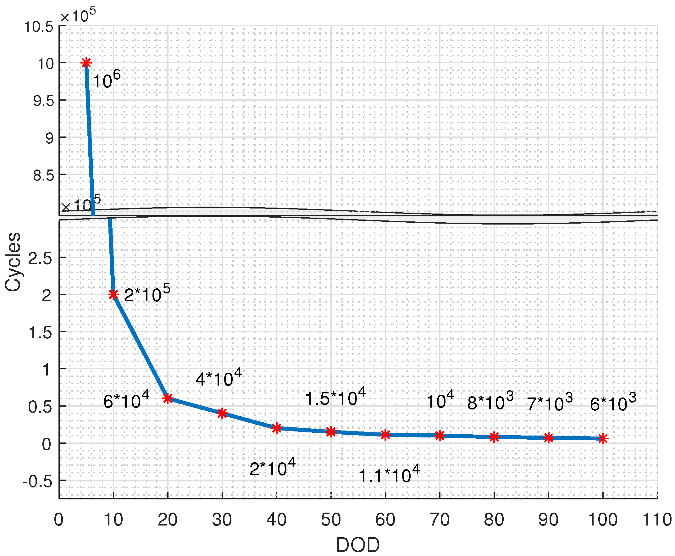
• The BESS daily degradation cost is computed as follows:

  $$De{g}_{cost,BESS}=\Delta SO{H}_{BESS}·K_{BESS},$$

  (10)

  where $De{g}_{cost,BESS}$ is the daily BESS degradation cost in EUR, and $K_{BESS}$ is the BESS replacement cost in EUR. The use of $K_{BESS}$ for computing a cost from battery degradation creates an optimization problem for amortizing a future BESS replacement.

2.2. Alkaline Electrolyzer

An AEL is a device that uses an alkaline electrolyte to split water into hydrogen and oxygen. The device is composed of an anode, cathode, and an ion-conductive membrane. When an electric voltage is applied across the electrodes, the water molecules at the anode are oxidized, releasing oxygen gas and protons. These protons then migrate through the diaphragm to the cathode, where they combine with electrons to form hydrogen gas [5].

Hydrogen is a valuable energy vector, with the potential for use as fuel for transportation or as an energy source for industrial applications. Since an AEL can convert electrical energy into this material, it allows for the integration of renewable energy plants into hydrogen markets. This provides a revenue stream for these energy generators [23]. When electricity prices are low, green hydrogen can be produced with generated energy or by purchases on the market.

The literature on AEL modeling is limited in comparison to the literature on BESS. A common approach is the use of current–voltage models, as first proposed by Ulleberg in [7]. However, these models are not efficient for long-range simulations due to their nonlinear nature and excessive complexity.

Authors in [24] introduce a model for mixed-integer dynamic optimization with a high degree of nonlinearity. In [25], the nonlinearities caused by the relationship between the modeling of heat production and electrolysis are dealt with. The framework proposed by authors in [25] uses an auxiliary advanced AEL model to update a fixed electrolysis efficiency in order to avoid nonlinearities and improve accuracy.

A linear formulation, suitable for MILP, is presented in [8]. This model incorporates operational states and startup times, which are very important in alkaline electrolyzers. The authors studied the effect of variable wind energy on power-to-hydrogen using a fluctuating wind energy source.

The model presented in this work is linear, its input variable is active power, and its output is hydrogen flow. The proposed model, which is an extension of the formulation presented in [8], considers degradation caused by usage and start/stop cycles. The effect of partial loads in $O_2$ purity is also incorporated.

Authors in [26] argue that the deterioration of the electrolyte is a result of the dissolution of elements, as well as the detachment and coalescence of catalysts. The degradation process results in a decline in efficiency, as reported in [27].

Nevertheless, there is a lack of empirical data for examining the AEL operation’s impact on this aging process. This makes the incorporation of degradation into AEL modeling less common. A fixed rate of 1% efficiency loss per year is considered in [28]. Authors in [27] follow a similar strategy.

The degradation model proposed in this work follows a semi-empirical approach, which gives an approximation of operation impact on loss of useful life. To quantify the degradation caused by intermittent operation, a start/stop cycle counter is utilized, as a limited number of cycles have been reported in [29]. Additionally, a working hours model is taken into account, recognizing that the loss of efficiency is also proportional to the limited lifetime hours, as reported in reference [30].

This semi-empirical model integrates manufacturer’s data about useful life into short-term operation analysis. As with the BESS model, the lost of useful lifetime by operation is computed using the units-of-production method [22]:

$$\Delta Lif{e}_{AEL}\left(t\right)=\frac{Hours\left(t\right)}{EO{L}_{hours}}+\frac{Cycles\left(t\right)}{EO{L}_{cycles}},$$

(11)

where:

• $Lif{e}_{AEL}\left(t\right)$: AEL remaining useful lifetime t (pu);
• Hours(t): Hours of operation during time period t;
• $EO{L}_{hours}$: Lifetime hours;
• Cycles(t): Start/stop cycles performed during time period t;
• $EO{L}_{cycles}$: Start/stop lifetime cycles.

Finally, the effect of partial loads on operation is considered. Hydrogen purity in oxygen decreases at lower current densities. This leads to the formation of explosive gases, as reported in [31]. After reaching a 2% $H_2$ concentration in $O_2$, the AEL is shut down as a safety measure.

In the approach outlined in [8], a minimal load threshold is established to control the purity of hydrogen in oxygen. This approach does not consider the contamination process at variable loads, which results in a less flexible operation. In this work, empirical data from [31] are used to develop an oxygen contamination model.

The results obtained by experiments conducted by authors in are depicted in Figure 3. As demonstrated in [31], at 25% of rated power, the 2% safety limit is reached in less than one hour. It is worth noting that this process is not reversible; once the limit is reached, the AEL needs to be shut down for purging. The oxygen contamination model proposed in this work computes the level of hydrogen purity based on the operational conditions, formulated as follows:

$$\Delta H_2\left(h\right)=\left\{\begin{array}{cc}3.5-5·P\left(h\right)\hfill & \mathrm{if}0.3\le P\left(h\right)\le 0.7\hfill \\ 0\hfill & \mathrm{if}P\left(h\right)>0.7\hfill \end{array}\right.,$$

(12)

where:

• $\Delta H_2\left(h\right)$: Hydrogen contamination growth during hour h (pu);
• P: AEL input power during hour h (pu).

Figure 3. Relationship between oxygen contamination and active power [31].

Figure 3. Relationship between oxygen contamination and active power [31].

The current approach employs the electrolyzer’s input power as a decision variable. The device generates hydrogen only at nominal pressure and temperature conditions [8]. Reaching and maintaining such conditions requires energy. In the absence of this energy, the device begins to cool, ultimately reaching a fully cold state. Consequently, the system’s operational modes are defined as follows:

• On mode: The AEL is producing hydrogen and operating at nominal conditions.
• Idle mode: Nominal conditions are maintained, but the AEL is not producing hydrogen.
• Off mode: The AEL is not generating hydrogen, and no energy is being applied to maintain nominal conditions, resulting in a gradual cooling until reaching a fully cold state.

These modes can be added to the formulation to increase the electrolyzer model’s accuracy by considering its operational behavior [32,33]. Transitioning from Off mode to On mode necessitates a starting energy proportional to the discrepancy between the electrolyzer’s current pressure and temperature and the conditions required for hydrogen production [34]. Both Off and Idle modes entail active power consumption, although power usage during Off mode is minimal. In this work, such power consumption is neglected.

As with the BESS model, the optimization constraints align with the physical limitations of the device, limiting the solution space. These constraints are outlined as follows:

• The total electrolyzer power output for each time period is derived from the sum of the various operating modes:

  $$P_{on}\left(t\right)+P_{idle}\left(t\right)+P_{start}\left(t\right)=P_{AEL}\left(t\right),$$

  (13)

  where $P_{on}\left(t\right)$ is the power employed in producing hydrogen during hour t in MW, $P_{idle}\left(t\right)$ is the power consumed in the Idle mode during hour t in MW, $P_{start}\left(t\right)$ is the cold starting power consumed during time period t in MW, and $P_{AEL}\left(t\right)$ is the total power consumption during hour t in MW.
• Binary variables are used to determine the AEL operation mode at each hour, and only one mode is allowed at a time:

  $${\pi }_{on}\left(t\right)+{\pi }_{off}\left(t\right)+{\pi }_{idle}\left(t\right)=1,$$

  (14)

  where ${\pi }_{on}\left(t\right)$ is the binary variable for On mode, ${\pi }_{off}\left(t\right)$ is the binary variable for Off mode, and ${\pi }_{idle}\left(t\right)$ is the binary variable for Idle mode. Each binary variable takes value 1 when its respective mode is enabled.
• An additional mode is used to define the cooling process, which appears only when the AEL is off:

  $$Cool\left(t\right)\le {\pi }_{off}\left(t\right),$$

  (15)

  where $Cool\left(t\right)$ is a binary variable that defines Cool mode, in which AEL temperature and pressure slowly decrease since it is shut down. It equals 1 when its temperature and pressure state has become colder.
• The pressure and temperature state of the electrolyzer is updated at each hour as follows:

  $$\tau \left(t\right)=\tau \left(t-1\right)+\upsilon \left(t\right)·t_{off}-Cool\left(t\right),$$

  (16)

  where $\tau \left(t\right)$ is the state at the end of hour t; this variable is limited between 0 and $t_{off}$. The variable $t_{off}$ is the number of hours it takes to get fully cold when off, and $\upsilon \left(t\right)$ is the fraction of the starting power required for a cold start.
• Whenever the electrolyzer is off, its temperature and pressure decrease until they reach the fully cold state:

  $$\left\{\begin{array}{c}Cool\left(t\right)\le \frac{\tau \left(t-1\right)}{t_{off}}+1\hfill \\ Cool\left(t\right)\ge \frac{\tau \left(t-1\right)}{t_{off}}-1+{\pi }_{off}\left(t\right)\hfill \end{array}\right.,$$

  (17)

  where the value 1 in the first term prevents the binary variable $Cool\left(t\right)$ from reaching a value of 0 until $\frac{\tau \left(t-1\right)}{t_{off}}$ is 0.
• Idle mode’s hourly power consumption is defined as:

  $$P_{idle}={\pi }_{idle}\left(t\right)·P_{idle},$$

  (18)

  where $P_{idle}$ is the hourly power consumption during Idle mode in MW.
• On mode’s hourly power consumption is limited as:

  $$P_{on,min}·{\pi }_{on}\left(t\right)\le P_{on}\left(t\right)\le P_{on,max}·{\pi }_{on}\left(t\right),$$

  (19)

  where $P_{on,min}$ and $P_{on,max}$ are the minimum and maximum AEL On mode’s active powers, respectively, in MW.
• The cold start power factor is defined as:

  $$\upsilon \left(t\right)\le \frac{t_{off}\left(t\right)-\tau \left(t-1\right)}{t_{off}}.$$

  (20)
  This factor, bounded between 0 and 1, represents how far the AEL is from reaching an operational state. If 1, it needs the full cold start power.
• The cold start power consumption is defined as:

  $$P_{start}\left(t\right)=\upsilon \left(t\right)·t_{start}·AE{L}_{Pmax},$$

  (21)

  where $P_{start}\left(t\right)$ is the AEL starting power in MW, $t_{start}$ is the cold start time in hours, and $AE{L}_{Pmax}$ is the maximum electrolyzer power in MW. This equation models the starting power consumption and considers that less power is required if the AEL is not completely cold when a cold start takes place.
• The hydrogen generation process is defined as:

  $$Q\left(t\right)=P_{on}·\frac{AE{L}_{eff}}{HHV},$$

  (22)

  where $Q\left(t\right)$ is the hydrogen flow during hour t in kg, $AE{L}_{eff}$ is the AEL efficiency in pu, and $HHV$ is the hydrogen high heating value in kg/MWh.
• The operation cost of the AEL, defined by the degradation models described above, is formulated as:

  $$De{g}_{Cost,AEL}\left(t\right)=\left(\frac{{\pi }_{on}\left(t\right)}{EO{L}_{hours}}+\frac{{\pi }_{off}(t-1)+{\pi }_{on}\left(t\right)+{\pi }_{idle}\left(t\right)-1}{EO{L}_{cycles}}\right)·K,$$

  (23)

  where $De{g}_{Cost,AEL}\left(t\right)$ is the degradation cost during hour t in EUR, and K is the electrolyzer replacement cost in EUR. The first term of the sum represents the degradation caused by operational hours of usage, and the second term is the degradation caused by on/off operational cycles.
• The oxygen contamination process is formulated as:

  $$imp\left(t\right)=imp\left(t-1\right)+cont\left(t\right)-2·purg\left(t\right),$$

  (24)

  where $imp\left(t\right)$ is the oxygen impurity level at the end of hour t in %, $cont\left(t\right)$ is the oxygen contamination during hour t in %, and $purg\left(t\right)$ is a binary variable that defines the AEL purging.
• The Purging mode is enabled when no $H_2$ is being produced:

  $$purg\left(t\right)\le {\pi }_{off}\left(t\right)+idle\left(t\right).$$

  (25)
  An inequality constraint is applied to allow for the possibility of Off and Idle modes to be non-zero when no purge is in progress. This scenario occurs, for instance, when the AEL is in a clean state and does not intend to generate hydrogen, enabling the Off or Idle binary variables to have a value of 1.
• When oxygen contamination reaches 2%, the AEL is shut down:

  $$imp\left(t-1\right)-{\pi }_{off}\left(t\right)\le 2.$$

  (26)
• Purging mode is disabled when the contamination value reaches 0:

  $$purg\left(t\right)\le imp(t-1).$$

  (27)
• A piecewise constraint is used to regulate the contamination process, derived from (12):

  $$cont\left(t\right)=\left\{\begin{array}{cc}0\hfill & \mathrm{if}\frac{P_{on}\left(t\right)}{AE{L}_{Pmax}}<0.3\hfill \\ 3.5-5·\frac{P_{on}\left(t\right)}{AE{L}_{Pmax}}\hfill & \mathrm{if}0.3\le \frac{P_{on}\left(t\right)}{AE{L}_{Pmax}}\le 0.7\hfill \\ 0\hfill & \mathrm{if}\frac{P_{on}\left(t\right)}{AE{L}_{Pmax}}>0.7\hfill \end{array}\right..$$

  (28)

2.3. Plant Model

The plant model illustrated in Figure 1 combines the previously formulated model constraints. Additional ones define the interactions between the plant components.

The system operates within the hydrogen and electricity markets. Energy generated by the wind turbine can be sent to the AEL, the BESS, and the grid. The BESS can supply energy to both the AEL and the grid. The AEL can receive energy from all other agents.

These additional constraints are used to determine the aforementioned interactions. Active powers during each hourly period are considered constant; thus, active power can be treated as energy. These constraints are defined as follows:

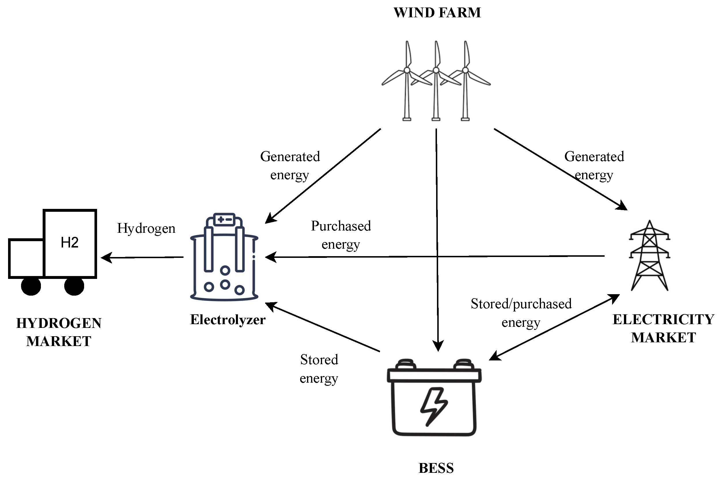
• The power generated by the wind farm is defined as:

  $$P_{gen}\left(t\right)=P_{WTG,BESS}\left(t\right)+P_{WTG,Grid}\left(t\right)+P_{WTG,AEL}\left(t\right)+P_{WTG,Curt}\left(t\right),$$

  (29)

  where $P_{gen}\left(t\right)$ is the generated power during hour t in MW, $P_{WTG,BESS}\left(t\right)$ is the generated power used by the BESS during hour t in MW, $P_{WTG,Grid}\left(t\right)$ is the generated power sent to the grid during hour t, $P_{WTG,AEL}\left(t\right)$ is the generated power sent to the AEL during hour t in MW, and $P_{WTG,Curt}\left(t\right)$ is the curtailed power during hour t in MW.
• The BESS discharging power is divided as follows:

  $$P_D\left(t\right)=P_{BESS,Grid}\left(t\right)+P_{BESS,AEL}\left(t\right),$$

  (30)

  where $P_{BESS,Grid}\left(t\right)$ is the BESS power sent to the grid during hour t in MW, and $P_{BESS,AEL}\left(t\right)$ is the BESS power sent to the AEL during hour t.
• The AEL power flow is defined as follows:

  $$P_{AEL}\left(t\right)=P_{BESS,AEL}\left(t\right)+P_{Grid,AEL}\left(t\right)+P_{WTG,AEL}\left(t\right).$$

  (31)

3. Mathematical Programming Models for Day-Ahead Market Bidding and Real-Time Control

The constraints from the previous section are applied in two optimization models. The first one consists of generating day-ahead electricity market commitments using wind speed electricity price forecasts while also generating hydrogen. The second model aims to reduce deviations in market commitments caused by forecast errors and to produce hydrogen from surplus electricity. This is illustrated in Figure 4.

In this section, the formulations of the objective functions of both models are introduced. As an example, the operation for a single day is shown. In this work, Cbc solver has been used in the optimization algorithm with a tolerance of ${10}^{-7}$.

3.1. Day-Ahead Market Bidding

This optimization model receives as inputs the hourly prices forecasts and the wind speed forecast. This model generates hourly day-ahead market commitments. Its objective function is formulated as follows:

$$\begin{array}{c}\mathrm{maximize}\sum _{t=1}^{24}[{\pi }_{el,fore}\left(t\right)·\left(P_{WTG,Grid}\left(t\right)+P_{BESS,Grid}\left(t\right)-P_{Grid,BESS}\left(t\right)-P_{Grid,AEL}\left(t\right)\right)\hfill \\ \hfill +{\pi }_{H2}·Q\left(t\right)-De{g}_{Cost,AEL}\left(t\right)]-De{g}_{Cost,BESS},\end{array}$$

(32)

where ${\pi }_{el,fore}\left(t\right)$ is the hourly forecasted electricity price in EUR/MWh, and ${\pi }_{H2}$ is the hydrogen price in EUR/kg. As can be seen, the objective function has two terms: one for the operation in the electricity market and the other for the operation in the hydrogen market.

3.2. Real-Time Operation

An optimization model is used to allocate resources to minimize deviation and maximize revenues by also producing hydrogen. An additional constraint, which calculates deviation costs, needs to be added to this model:

$$De{v}_{Costs}\left(t\right)=[P_{Com,DM}\left(t\right)-\left(P_{WTG,Grid}\left(t\right)-P_{BESS,Grid}\left(t\right)\right)]·\lambda ·{\pi }_{el,real}\left(t\right),$$

(33)

where $P_{Com,DM}\left(t\right)$ is the day-ahead market power commitment for hour t in MW, ${\pi }_{el,real}\left(t\right)$ is the real electricity price for hour t in EUR/MWh, and $\lambda$ is the deviation cost factor for hour t. The objective function of this optimization problem is formulated as follows:

$$maximize\sum _{t=1}^{24}[{\pi }_{H2}·Q\left(t\right)-De{v}_{Costs}\left(t\right)]-De{g}_{cost}\left(t\right).$$

(34)

The primary objective at this stage is to optimize profits through the implementation of measures aimed at minimizing deviation costs and utilizing surplus energy for the production of hydrogen.

4. Two-Stage Stochastic Optimization Algorithm

A two-stage stochastic problem is developed using the aforementioned optimization models. This section provides an overview of these stochastic algorithms and their application. The standard Monte Carlo simulation approach is presented. Afterwards, an algorithm based on bootstrap sampling is proposed.

4.1. Two-Stage Stochastic Optimization Overview

This mathematical framework involves making decisions in two stages. In the first stage, a decision is made by solving the optimization problem based on the available information. This can be done by using a deterministic forecast as input, and the solution generated is called the candidate solution [35].

Then, the outcome of the candidate solution is evaluated in the second stage. At this stage, the cost of the decisions made in the first are computed using the realization of the uncertain parameters. The best solution is evaluated using both the expected benefits in the first stage and the cost in the second one. The optimization model aims to reduce the cost of the second-stage decisions while selecting the candidate solution with the highest first-stage benefits.

Two-stage optimization problems can be used in EMS applications [9]. In this work, the first stage involves the day-ahead optimization, while the second stage is the real-time operation. It is common to employ sets of scenarios to generate different candidates and evaluate their second-stage costs under different situations [36].

4.2. Monte Carlo Approach

Monte Carlo simulation is a statistical method that utilizes random sampling to generate multiple sets of possible outcomes for a given problem [37]. This method is particularly useful in two-stage stochastic optimization, as it allows for the estimation of the probability of the outcome of the first-stage decisions.

The scenarios, generated using historical data in the forecasting model, are used to obtain a probability density function of the realization of the uncertain parameters. A set of 10 wind speed and electricity price scenarios for 25 March 2020 is shown in Figure 5, for both wind speed and electricity prices. This number of scenarios is employed because a higher number would exponentially increase computational burden.

For each combination of scenarios, a candidate solution is generated using the day-ahead optimization model. Therefore, in the first stage, 100 candidate solutions are generated. The power commitments of each candidate solution are sent to the real-time optimization model.

The real-time optimization is solved for each candidate solution under each wind and price scenario. The costs of each candidate under each combination of scenarios are calculated as follows:

$$Cost{(i,j)}_x=De{v}_{Costs}(i,j)+\Delta E_{Ben}(i,j),$$

(35)

where $Cost{(i,j)}_x$ represents the second-stage costs under wind speed scenario j and electricity price scenario i for candidate solution x in EUR. $De{v}_{Costs}(i,j)$ are the deviation costs in EUR, and $\Delta E_{Ben}(i,j)$ is the difference between expected and real electricity market benefits in EUR.

A sample of 100 second-stage costs is generated for each candidate solution. Figure 6 illustrates an example.

As can be seen, negative costs result from certain combinations of scenarios, indicating more energy was available than expected. The accuracy of Monte Carlo-based stochastic algorithms depends on the number of simulations, so a large number of simulations should be performed to reduce uncertainty in the results. This stochastic optimization problem can be formulated as follows [38]:

$$max{E}_1\left(S\right)-CVa{R}_{1-\beta }\left(E_2\left(S\right)\right),$$

(36)

where $E_1\left(S\right)$ are the expected benefits for candidate solution S in EUR, and $CVa{R}_{1-\beta }\left(E_2\left(S\right)\right)$ is the conditional value-at-risk of the second-stage costs for candidate solution S in EUR for the confidence interval $\beta$, which has been set to 95%, a common choice in stochastic problems.

The current implementation faces a challenge in regards to increasing the number of available samples. Each sample requires solving an additional optimization problem, and therefore, for 100 candidate solutions, 10,000 optimization problems must be solved for each day. This can result in the requirement to solve one million optimization problems in order to obtain 1000 samples for 1000 candidate solutions, which may render the problem computationally infeasible due to the amount of computational time required, especially considering that this model runs online.

4.3. Bootstrapping Approach

Bootstrapping is a re-sampling method that allows us to estimate parameters using sampled data [39]. It is used when the sampling process is difficult, such as in clinical studies [40]. It is also used when the available input data are scarce, which is the common case in some forecasting applications [41].

This method involves re-sampling the original population randomly, thereby generating a new sample. A statistical quantity of the new sample is calculated, such as the mean. By repeating this process, a distribution of estimates is obtained, which can be used to calculate variability measures.

Bootstrapping is often computationally simpler than Monte Carlo. Additionally, it can provide more accurate estimates when the sample size is small or the distribution is not normal. Also, obtaining a confidence interval of a statistical quantity allows for a more robust approach with a smaller population of samples.

In this application, the mean of the re-samples is used in the bootstrap process. The original population is re-sampled 10,000 times, and repetition is allowed. An example of a bootstrap sample for the second-stage costs is shown in Figure 7.

As can be seen, this distribution presents a more normal shape. The formulation presented in (36) can be adapted to this approach as follows:

$$max{E}_1\left(S\right)-CVa{R}_{1-\beta }\left(E_2\left(\overline{S}\right)\right),$$

(37)

where $CVa{R}_{1-\beta }\left(E_2\left(\overline{S}\right)\right)$ is the conditional value-at-risk of the second-stage cost means for candidate solution S in EUR for the confidence interval $\beta$. A 95% confidence interval is used in this case.

5. Simulation Framework and Results

A demonstration of the introduced model is presented in this section. Afterwards, the simulation framework for evaluating the performance of the proposed optimization method is described. Different simulation scenarios are run on the same plant model, and in each case, a different approach for generating day-ahead market commitments is considered. Results under each approach are presented and compared. The key performance indicators considered are the earnings for both electricity and hydrogen markets.

5.1. Single-Day Demonstration

This subsection presents a demonstration of the formulated plant model operation for 25 March 2020. The demonstration employs a deterministic forecast of electricity prices and generated power as input for the day-ahead stage. The power commitments are subsequently input into the real-time optimization problem, the primary objective of which is to minimize deviation resulting from forecasting errors.

The plant’s component parameters are introduced in

Table 1. Plant parameters.

Parameter	Value	Parameter	Value
AEL Nominal Power	1 MW	AEL Cooling Time	5 h
AEL Minimum Power	0.3 MW	Hydrogen HHV	0.0394 kg·MW
AEL Efficiency	75%	AEL Idle Mode Power	0.04 MW
AEL Replacement Cost	500 EUR/kW	BESS Capacity	10 MWh
AEL Lifetime	100,000 h	BESS Nominal Power	2.5 MW
AEL Lifetime Cycles	50,000	BESS Efficiency	90%
AEL Cold Start Time	12 min	BESS Replacement Cost	50 EUR/KWh

.

Historical electricity prices in DKK are used as input for the forecasting model. The authors in [42] statistically show that a SARIMA with order $(2,1,3){(1,0,1)}_{24}$ is appropriate for forecasting such prices, and the same order is used here. The previous 100 days of hourly electricity prices are used as training data.

Hourly wind speed data, obtained from the Merra-2 Database [43] located in Brande, Denmark, are used as input for wind speed prediction. In its first stage, a SARIMA model is used to generate a deterministic forecast of wind speed, which is then computed as wind power using the curve of the Siemens SWT-3.0-113 wind turbine generator. The SARIMA model has an order of $(2,0,1){(2,0,3)}_{12}$. Wind speed data from the previous five days are used as training data.

In Figure 8, deterministic forecasts for price and wind speed on 25 March 2020 are shown. This day has been selected arbitrarily for illustration purposes. The figure shows that forecast errors grow over time, with electricity prices overestimated in later hours and wind speed underestimated for this specific day.

The inputs for the day-ahead scheduling optimization problem are the predicted wind and electricity prices, as shown in Figure 8. The optimal solution is depicted in Figure 9, which shows the hourly active power from the plant components and the power exchanges with the grid.

The electrolyzer starts at full power later in the first hour by taking cold start power from the grid and runs at full power all day. The battery schedules an arbitrage operation using the price spread. When electricity prices are low, some power generated from the wind turbine is sent to the electrolyzer for hydrogen production.

The hourly commitments generated in this stage are sent to the real-time stage. The optimization problem takes as input the real electricity prices, as well as the wind speed from day and day-ahead hourly power commitments. Figure 10 illustrates these results.

The optimization problem uses the BESS to cover deviations since real generated power is lower than expected (as shown in Figure 8). Wind turbine generated power is stored during low electricity price hours, when deviation costs are low, and released by the BESS during price peaks at the end of the day. Hydrogen production is kept constant during the day.

5.2. Case Studies

Different case studies are performed with the simulation framework. The simulation is run from 1 January 2020 to 31 December 2020. AEL and BESS states at the end of a day are considered as the initial state for the next one. For simplicity, perfect price and wind power foresight are assumed.

5.2.1. Hydrogen Price Effects on Market Participation

The plant participates in two different markets, but future hydrogen prices are uncertain. The first case study examines the effects of various hydrogen prices. Figure 11 illustrates the accumulated benefits at the end of the year attained in both electricity and hydrogen markets.

The figure shows that the hydrogen market benefits become noticeable only when hydrogen prices exceed 1.5 EUR per kg. As the hydrogen prices increase further, the plant starts to use more energy for hydrogen production and, as a result, the electricity market participation decreases. When the hydrogen price reaches 3.5 EUR/kg, the benefits from the hydrogen market surpass the ones from the electricity market. It is remarkable how the benefits of hydrogen market start to appear only after a certain threshold.

5.2.2. Hydrogen Price Effects on Different Hydrogen Off-Taker Scenarios

Various green hydrogen supply chain configurations exist. One option involves a pipeline infrastructure, where the plant unloads the produced hydrogen in real time [44]. Another option, particularly in the case of remote plant locations such as offshore locations, involves the storage of hydrogen in a tank, which is unloaded periodically using trucks or vessels [45], adding an extra constraint to green hydrogen production.

In this case study, different tank capacities and different tank unloading schedules are evaluated, and scenarios of low and high hydrogen prices are considered. Moreover, the scenario of a hydrogen pipeline is also evaluated. Figure 12 illustrates the accumulated benefits at the end of the year in each case.

Results demonstrate how the pipeline scenario yields the best results. Increasing tank unloading regularity permits operating with smaller tanks. This constraint needs to be carefully considered when sizing the plant in order to obtain the best balance between unloading schedule and tank capacity. This requirement is present in both low-price and high-price scenarios; however, the presence of a pipeline clearly demonstrates better results in any case.

5.2.3. Hydrogen Price Effects Depending on AEL Grid Connections

The AEL interacts with the electricity market, as shown in Figure 1, enabling the purchase of energy from the market to produce hydrogen when electricity prices are low. The final case study examines the impact of the plant’s participation in both markets at different hydrogen prices.

A base case is considered in which hydrogen market participation is disabled, and therefore benefits are only obtained from the electricity market. Two options for hydrogen market participation are evaluated: one in which the AEL is connected to the grid and another in which it is disconnected from the grid, so its input power is only obtained from wind production. Accumulated benefits in each case are illustrated in Figure 13.

Results indicate that, at low hydrogen prices, enabling hydrogen market participation increases plant outcome only when the AEL is disconnected from the grid. AEL interaction with the electricity market only yields better results when hydrogen prices approach 3 EUR/kg, indicating that only high hydrogen prices justify the connection to the grid.

5.3. Stochastic Algorithm Comparison

In order to compare the proposed stochastic optimization model, a simulation framework of the plant participating in hydrogen and day-ahead electricity markets is developed, and a hydrogen price of 4 EUR/kg is considered. The plant component parameters are the ones depicted in Table 1.

Four different simulation scenarios are considered:

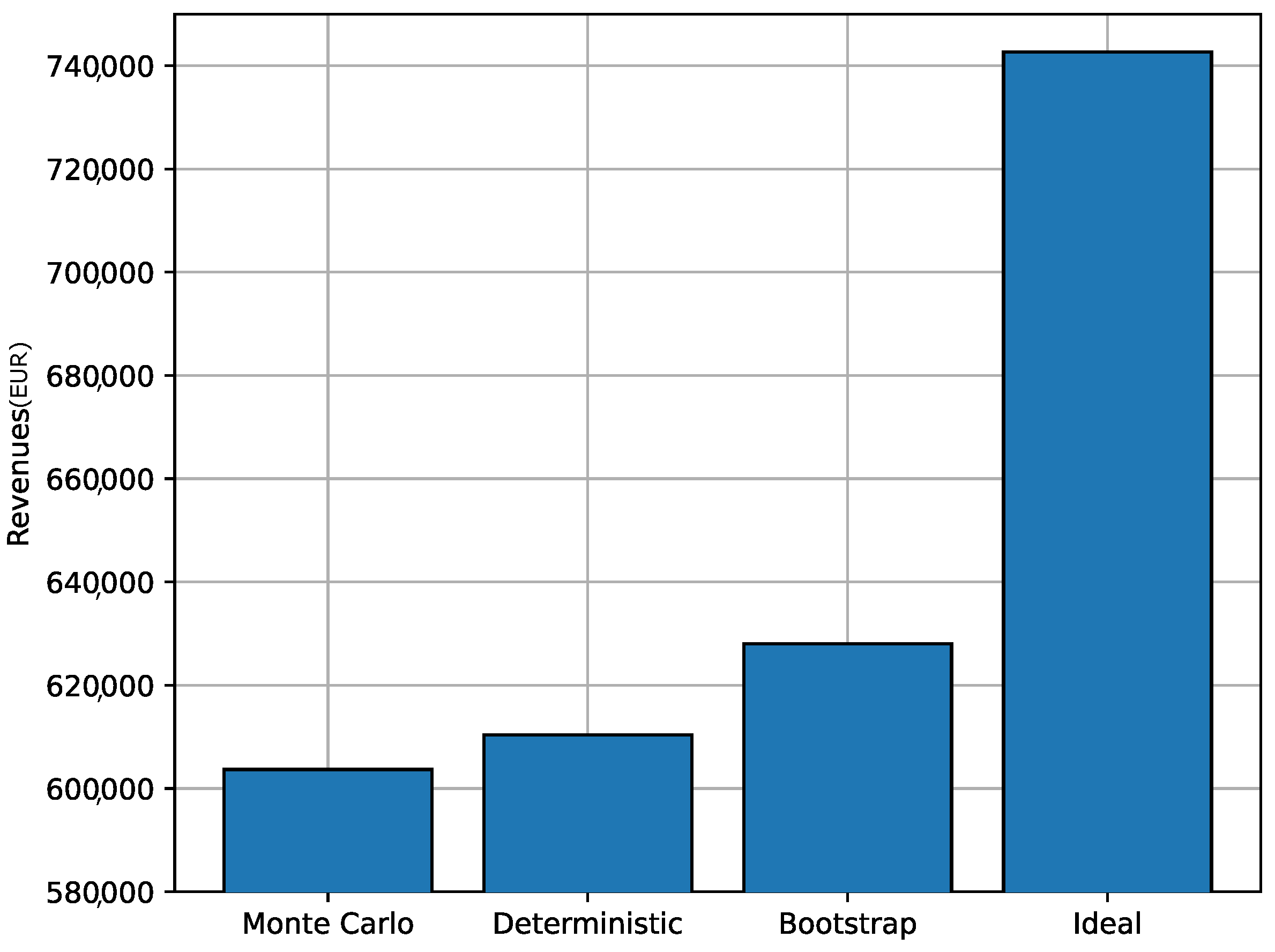
• Ideal scenario: The plant receives perfect wind speed and electricity price forecasts.
• Stochastic Monte Carlo scenario: The Monte Carlo algorithm is used for day-ahead commitment generation.
• Stochastic Bootstrap scenario: The proposed bootstrap algorithm is used for day-ahead commitment generation.
• Deterministic scenario: A direct approach that considers deterministic forecasts.

The simulation is run from 1 January 2020 to 31 December 2020. The revenues have been calculated using historical prices in DKK for each day. The total revenues for each simulation case are presented in Figure 14.

The Deterministic method of utilizing direct predictions surpasses the utilization of the conventional Monte Carlo technique. This can be caused by the low amount of available scenarios. The strategy that has been proposed, incorporating bootstrap sampling, demonstrates superior results compared to both the Monte Carlo and Deterministic approaches.

6. Conclusions and Future Work

A mathematical optimization model has been proposed for the integration of an AEL, a BESS, and a wind turbine generator. This model takes into account the effect of partial loading into the AEL oxygen phase, as well as the degradation effects for both the AEL and the BESS. A linear formulation has been proposed to ensure its efficiency in EMS optimization applications.

The effect of wind speed and energy price uncertainties has been addressed with the proposal of a two-stage stochastic optimization model. The state-of-the-art Monte Carlo approach has been compared to a novel bootstrap-based algorithm. A simulation framework has been developed to evaluate the performance of the proposed algorithm.

A comparison between a classical Monte Carlo approach and the proposed bootstrapping implementation demonstrates how this algorithm yields a better outcome than the use of a Monte Carlo strategy using the same data. This can be useful for online applications, in which computational time is a constraint for continuous operation.

Case studies of different plant configurations and hydrogen supply chain structures have been studied. Results demonstrate how, at low hydrogen prices, plant configuration must be carefully addressed in order to obtain optimal income. Moreover, AEL interactions with the electrical market are detrimental at low hydrogen prices.

In future work, the authors propose an extension of this algorithm for intra-day market participation. The BESS participation in frequency response services is also suggested. Also, it is considered that some limitations, such as testing longer time frames or different electricity markets, could be considered for future research.

References

- Renewable Capacity Statistics 2023. 2023. Available online: https://www.irena.org/Publications/2023/Mar/Renewable-capacity-statistics-2023 (accessed on 21 January 2024).
- Kalair, A.; Abas, N.; Saleem, M.S.; Kalair, A.R.; Khan, N. Role of energy storage systems in energy transition from fossil fuels to renewables. Energy Storage 2021, 3, e135. [Google Scholar] [CrossRef]
- Dogger, J.D.; Roossien, B.; Nieuwenhout, F.D.J. Characterization of Li-Ion Batteries for Intelligent Management of Distributed Grid-Connected Storage. IEEE Trans. Energy Convers. 2011, 26, 256–263. [Google Scholar] [CrossRef]
- Abbasi, T.; Abbasi, S. ‘Renewable’ hydrogen: Prospects and challenges. Renew. Sustain. Energy Rev. 2011, 15, 3034–3040. [Google Scholar] [CrossRef]
- Bodner, M.; Hofer, A.; Hacker, V. H2 generation from alkaline electrolyzer. WIREs Energy Environ. 2015, 4, 365–381. [Google Scholar] [CrossRef]
- Reniers, J.M.; Mulder, G.; Ober-Blöbaum, S.; Howey, D.A. Improving optimal control of grid-connected lithium-ion batteries through more accurate battery and degradation modelling. J. Power Sources 2018, 379, 91–102. [Google Scholar] [CrossRef]
- Ulleberg, Ø. Modeling of advanced alkaline electrolyzers: A system simulation approach. Int. J. Hydrogen Energy 2003, 28, 21–33. [Google Scholar] [CrossRef]
- Varela, C.; Mostafa, M.; Zondervan, E. Modeling alkaline water electrolysis for power-to-x applications: A scheduling approach. Int. J. Hydrogen Energy 2021, 46, 9303–9313. [Google Scholar] [CrossRef]
- Roald, L.A.; Pozo, D.; Papavasiliou, A.; Molzahn, D.K.; Kazempour, J.; Conejo, A. Power systems optimization under uncertainty: A review of methods and applications. Electr. Power Syst. Res. 2023, 214, 108725. [Google Scholar] [CrossRef]
- Eghbali, N.; Hakimi, S.M.; Hasankhani, A.; Derakhshan, G.; Abdi, B. Stochastic energy management for a renewable energy based microgrid considering battery, hydrogen storage, and demand response. Sustain. Energy Grids Netw. 2022, 30, 100652. [Google Scholar] [CrossRef]
- Yu, D.; Wang, J.; Li, D.; Jermsittiparsert, K.; Nojavan, S. Risk-averse stochastic operation of a power system integrated with hydrogen storage system and wind generation in the presence of demand response program. Int. J. Hydrogen Energy 2019, 44, 31204–31215. [Google Scholar] [CrossRef]
- Abdelghany, M.B.; Al-Durra, A.; Zeineldin, H.; Hu, J. Integration of cascaded coordinated rolling horizon control for output power smoothing in islanded wind–solar microgrid with multiple hydrogen storage tanks. Energy 2024, 291, 130442. [Google Scholar] [CrossRef]
- Abdelghany, M.B.; Al-Durra, A.; Daming, Z.; Gao, F. Optimal multi-layer economical schedule for coordinated multiple mode operation of wind–solar microgrids with hybrid energy storage systems. J. Power Sources 2024, 591, 233844. [Google Scholar] [CrossRef]
- McMurry, J.; Fay, R.C.; Robinson, J.K. Chemistry; Pearson: London, UK, 2015. [Google Scholar]
- Rosewater, D.M.; Copp, D.A.; Nguyen, T.A.; Byrne, R.H.; Santoso, S. Battery Energy Storage Models for Optimal Control. IEEE Access 2019, 7, 178357–178391. [Google Scholar] [CrossRef]
- Barré, A.; Deguilhem, B.; Grolleau, S.; Gérard, M.; Suard, F.; Riu, D. A review on lithium-ion battery ageing mechanisms and estimations for automotive applications. J. Power Sources 2013, 241, 680–689. [Google Scholar] [CrossRef]
- Maheshwari, A.; Paterakis, N.G.; Santarelli, M.; Gibescu, M. Optimizing the operation of energy storage using a non-linear lithium-ion battery degradation model. Appl. Energy 2020, 261, 114360. [Google Scholar] [CrossRef]
- Cao, J.; Harrold, D.; Fan, Z.; Morstyn, T.; Healey, D.; Li, K. Deep Reinforcement Learning-Based Energy Storage Arbitrage With Accurate Lithium-Ion Battery Degradation Model. IEEE Trans. Smart Grid 2020, 11, 4513–4521. [Google Scholar] [CrossRef]
- Ouyang, D.; Weng, J.; Chen, M.; Liu, J.; Wang, J. Experimental analysis on the degradation behavior of overdischarged lithium-ion battery combined with the effect of high-temperature environment. Int. J. Energy Res. 2020, 44, 229–241. [Google Scholar] [CrossRef]
- Doerffel, D.; Sharkh, S.A. A critical review of using the Peukert equation for determining the remaining capacity of lead-acid and lithium-ion batteries. J. Power Sources 2006, 155, 395–400. [Google Scholar] [CrossRef]
- Cheng, S.; Liu, Y.H.; Hesse, H.; Naumann, M.; Truong, C.; Jossen, A. A PSO-Optimized Fuzzy Logic Control-Based Charging Method for Individual Household Battery Storage Systems within a Community. Energies 2018, 11, 469. [Google Scholar] [CrossRef]
- Wang, Y.; Zhou, Z.; Botterud, A.; Zhang, K.; Ding, Q. Stochastic coordinated operation of wind and battery energy storage system considering battery degradation. J. Mod. Power Syst. Clean Energy 2016, 4, 581–592. [Google Scholar] [CrossRef]
- Oliveira, A.M.; Beswick, R.R.; Yan, Y. A green hydrogen economy for a renewable energy society. Curr. Opin. Chem. Eng. 2021, 33, 100701. [Google Scholar] [CrossRef]
- Niaz, H.; Liu, J. A Mixed Integer Dynamic Optimization Approach for a Hybrid-Stand Alone Solar and Wind Powered Alkaline Water Electrolyser for Renewable Hydrogen. In 31st European Symposium on Computer Aided Process Engineering; Türkay, M., Gani, R., Eds.; Elsevier: Amsterdam, The Netherlands, 2021; Volume 50, pp. 1285–1291. [Google Scholar]
- Huang, C.; Zong, Y.; You, S.; Træholt, C. Economic model predictive control for multi-energy system considering hydrogen-thermal-electric dynamics and waste heat recovery of MW-level alkaline electrolyzer. Energy Convers. Manag. 2022, 265, 115697. [Google Scholar] [CrossRef]
- Lafforgue, C.; Zadick, A.; Dubau, L.; Maillard, F.; Chatenet, M. Selected Review of the Degradation of Pt and Pd-based Carbon-supported Electrocatalysts for Alkaline Fuel Cells: Towards Mechanisms of Degradation. Fuel Cells 2018, 18, 229–238. [Google Scholar] [CrossRef]
- David, M.; Ocampo-Martínez, C.; Sánchez-Peña, R. Advances in alkaline water electrolyzers: A review. J. Energy Storage 2019, 23, 392–403. [Google Scholar] [CrossRef]
- Ali Khan, M.H.; Daiyan, R.; Han, Z.; Hablutzel, M.; Haque, N.; Amal, R.; MacGill, I. Designing optimal integrated electricity supply configurations for renewable hydrogen generation in Australia. iScience 2021, 24, 102539. [Google Scholar] [CrossRef] [PubMed]
- Brauns, J.; Turek, T. Alkaline Water Electrolysis Powered by Renewable Energy: A Review. Processes 2020, 8, 208. [Google Scholar] [CrossRef]
- Schmidt, O.; Gambhir, A.; Staffell, I.; Hawkes, A.; Nelson, J.; Few, S. Future cost and performance of water electrolysis: An expert elicitation study. Int. J. Hydrogen Energy 2017, 42, 30470–30492. [Google Scholar] [CrossRef]
- Fang, R.; Liang, Y. Control strategy of electrolyzer in a wind-hydrogen system considering the constraints of switching times. Int. J. Hydrog. Energy 2019, 44, 25104–25111, Special Issue on International Conference on Novel Functional Materials 2018. [Google Scholar] [CrossRef]
- Shehzad, M.F.; Abdelghany, M.B.; Liuzza, D.; Glielmo, L. Modeling of a Hydrogen Storage Wind Plant for Model Predictive Control Management Strategies. In Proceedings of the 2019 18th European Control Conference (ECC), Naples, Italy, 25–28 June 2019; pp. 1896–1901. [Google Scholar]
- Abdelghany, M.B.; Al-Durra, A. A coordinated model predictive control of grid-connected energy storage systems. In Proceedings of the 2023 American Control Conference (ACC), San Diego, CA, USA, 31 May–2 June 2023; pp. 1862–1867. [Google Scholar]
- Matute, G.; Yusta, J.; Beyza, J.; Correas, L. Multi-state techno-economic model for optimal dispatch of grid connected hydrogen electrolysis systems operating under dynamic conditions. Int. J. Hydrogen Energy 2021, 46, 1449–1460. [Google Scholar] [CrossRef]
- Ruszczynski, A.; Shapiro, A. Handbooks in OR & MS, Vol. 10; Elsevier Science B.V.: Amsterdam, The Netherlands, 2003. [Google Scholar]
- Qiu, H.; Gu, W.; Liu, P.; Sun, Q.; Wu, Z.; Lu, X. Application of two-stage robust optimization theory in power system scheduling under uncertainties: A review and perspective. Energy 2022, 251, 123942. [Google Scholar] [CrossRef]
- Harrison, R.L. Introduction to Monte Carlo Simulation. AIP Conf. Proc. 2010, 1204, 17–21. [Google Scholar] [PubMed]
- Lan, P.; Han, D.; Zhang, R.; Xu, X.; Yan, Z. Optimal portfolio design of energy storage devices with financial and physical right market. Front. Energy 2021, 16, 95–104. [Google Scholar] [CrossRef]
- Efron, B.; Tibshirani, R. An Introduction to the Bootstrap; Chapman & Hall/CRC: Boca Raton, FL, USA, 1993. [Google Scholar]
- Rosenfeld, J.P.; Donchin, E. Resampling (bootstrapping) the mean: A definite do. Psychophysiology 2015, 52, 969–972. [Google Scholar] [CrossRef] [PubMed]
- Hasni, M.; Aguir, M.; Babai, M.; Jemai, Z. Spare parts demand forecasting: A review on bootstrapping methods. Int. J. Prod. Res. 2019, 57, 4791–4804. [Google Scholar] [CrossRef]
- McHugh, C.; Coleman, S.; Kerr, D.; McGlynn, D. Forecasting Day-ahead Electricity Prices with A SARIMAX Model. In Proceedings of the 2019 IEEE Symposium Series on Computational Intelligence (SSCI), Xiamen, China, 6–9 December 2019; pp. 1523–1529. [Google Scholar] [CrossRef]
- Global Modeling and Assimilation Office. inst3_3d_asm_Cp: MERRA-2 3D IAU State, Meteorology Instantaneous 3-Hourly (p-coord, 0.625x0.5L42), Version 5.12.4. 2015. Available online: https://gmao.gsfc.nasa.gov/reanalysis/MERRA-2/data_access/ (accessed on 21 November 2022).
- Ball, M.; Wietschel, M. The future of hydrogen—Opportunities and challenges. Int. J. Hydrogen Energy 2009, 34, 615–627. [Google Scholar] [CrossRef]
- Seo, Y.; Park, H.; Lee, S.; Kim, J.; Han, S. Design concepts of hydrogen supply chain to bring consumers offshore green hydrogen. Int. J. Hydrogen Energy 2023, 48, 15126–15142. [Google Scholar] [CrossRef]