Article

Evaluating the Accuracy of Contour Ridgeline Positioning for Soil Conservation in the Northeast Black Soil Region of China

1
School of Geography and Environment, Liaocheng University, Liaocheng 252059, China
2
Liaocheng Innovative High Resolution Data Technology Co., Liaocheng 252059, China
3
Northeast Institute of Geography and Agroecology, Chinese Academy of Sciences, Harbin 150081, China
*
Author to whom correspondence should be addressed.
Sustainability 2024, 16(8), 3106; https://doi.org/10.3390/su16083106
Submission received: 29 February 2024 / Revised: 29 March 2024 / Accepted: 7 April 2024 / Published: 9 April 2024
(This article belongs to the Section Soil Conservation and Sustainability)

Abstract

:
The Northeast black soil region is China’s vital commercial grain base. However, severe soil erosion on slope farmland poses a significant threat to this region’s sustainable agricultural productivity. The transition from traditional downslope ridging to contour ridging (briefly referred to as “contour ridging”) is one of the primary sustainable measures for preventing soil erosion on slope farmland. By integrating high-precision Digital Elevation Models (DEMs) and design standards, ArcMap can plan the orientation and position of contour ridgelines and estimate the reduction in soil erosion on slope farmland after implementing contour ridging. Therefore, the degree of discrepancy between the designed and implemented positions of the contour ridgelines directly affects the effectiveness of contour ridging and the precision in evaluating its impacts and benefits. This study aims to assess the position accuracy of contour ridgelines designed by ArcMap 10.5 (here after ArcMap) using high-precision DEMs obtained from unmanned aerial vehicles (UAV). For this purpose, three fields where contour ridging had already been implemented were selected in the Sanjiang Plain of Heilongjiang Province, China. CORS RTK was used to measure the XYZ coordinates of verification points along implemented ridges precisely. Those measured coordinates were compared with the designed ridgeline positions to analyze the positional discrepancies between the designed and implemented ridgelines. The results indicated the following: (1) The average slope gradient along contour ridgelines measured in the field (0.5~0.6°) was relatively close to that along the ridgelines designed using ArcMap (0.6°), and the elevation changes along most of the contour ridgelines showed a pattern of being higher in the middle and lower on both sides. (2) The positional offset between most of the measured and designed ridgelines was less than the width of a single ridge (1.3 m), and the median offset was one-third of the width of a single ridge. (3) The positional offset caused by the movement of ridging machinery could be larger than the offset resulting from the baseline setup, and verification points with larger positional offsets were often located at the edges of the plots as well as turns of the ridgelines. Therefore, during the designing ridgelines process, the turns should be made as smooth as possible. During ridging, reducing the speed at these turns to minimize errors and maintain the accuracy of the ridgeline was recommended. The findings of this study can provide a scientific basis to improve contour ridging design and effect prediction in slope farmland to control soil erosion and enhance agricultural sustainability.

Graphical Abstract

1. Introduction

The Northeast Black Soil Region noted for its fertile chernozem, is crucial in ensuring China’s food security [1]. It contributes one-third of the country’s commercial grain supply, acting as a stabilizing force for national food security [2]. However, over a century of intensive exploitative management and lack of proper conservation [3] have led to severe degradation of the black soil, posing a threat to the country’s food security. The average thickness of the black soil layer in this region has decreased from 60–80 cm in the 1950s to 20–40 cm today [4]. Erosion of 30 cm from the black soil topsoil can result in a nearly 50% decrease in soybean yield [5]. Additionally, (shallow) gullies mainly developed in slope farmland in this region, causing fragmentation of the arable land and efficiency reduction of agricultural machinery [6,7]. Therefore, preventing and controlling soil and water erosion in the slope farmland [8] of the Black Soil Region is essential for preserving the black soil and enhancing sustainable grain production capacity.
Traditional downslope ridging is the primary cultivation measurement on the slope farmland in the Northeast black soil region of China. Although this measurement can quickly drain rainwater and melting snow runoff from slope farmland [9], the resulting “ridge-gully” system also accelerates soil erosion [10]. Adjusting traditional downslope ridging to contour or cross-slope ridging (from now on referred to as “contour ridging”) is an essential measure for managing soil erosion in slope farmland [11]. The benefits of contour ridging in preventing soil and water erosion, increasing soil organic matter content [12], and reducing non-point source pollution [13] have been validated through runoff plots and field experiments across various soil types and erosion-prone areas [14,15]. Compared with other slope farmland soil conservation measures such as subsoiling or crop rotation, contour farming could maintain agricultural productivity without additional agricultural machinery, making it an appropriate soil conservation strategy for slope farmland in this region. Considering its significant benefits and low investment requirements, the government has listed contour ridging as an essential measurement for black soil conservation.
Although the many advantages of contour ridging have been confirmed, improper design of this measurement could lead to more severe soil erosion than traditional downslope ridging [16,17]. Contour ridging works by intercepting surface runoff and delaying runoff generation on slope farmland, thus controlling soil loss caused by runoff erosion. However, its drainage effectiveness is weaker than downslope ridging, making it prone to water accumulation [18]. Due to variations in the micro-topography of slope farmland, an unreasonable design might create low points along the contour ridges. These low points can lead to waterlogging in autumn, reducing harvest efficiency [19]. During heavy rainfall, excessive water accumulation can cause overland flow and ridge breakage [20]. Hence, rational design is critical to ensure contour ridging works properly.
Most previous studies on contour ridging have focused on runoff plots, around 100 square meters in size [14,21]. Due to their small size, these plots typically have flat terrain with primarily straight-line contour ridging, making it easier to design the position and orientation of all ridgelines and achieve an ideal form of contour ridging. However, slope farmland in fields is larger in scale (several tens of hectares or more) and has uneven terrain, making implementing contour ridging within slope farmland more challenging. Most of the literature on field contour ridging focuses on post-implementation ecological benefits [22,23], with fewer reports on the design and effectiveness of contour ridging implementation.
The traditional design process for the baseline in contour ridging in northeast China usually applies a total station or RTK (Real Time Kinematic) to collect surface elevation data. This data, combined with the elevation change rules along the baseline, is used to design baseline locations. Ground markers or flags are placed at regular intervals (such as every 15 m) to establish the baseline. Once this layout process is complete, ridging machinery equipped with a navigation system travels along the baseline to acquire data on its direction. Subsequently, the navigation system guides the ridging process, allowing all farming activities to be performed parallel to that baseline. During the traditional design phase of the baseline, topographical maps or Digital Elevation Models (DEMs) of the slope farmland are used as reference data. Their primary purpose is to provide the general direction of the baseline. However, the traditional design process for contour ridging only calculates the primary direction of the contour ridges and the gradient along the baseline, neglecting the elevation changes and gradients along ridges within the remaining area in the field. This oversight can lead to low points within the remaining area due to minor undulations in the terrain, resulting in impractical contour ridging designs. The geographic information system software platform, such as ArcMap, has a feature for translating (or shifting) linear features, which allows the baseline to be moved at set intervals within the remaining area of the slope farmland [24,25]. The high-precision DEM obtained by drones can reflect the fine elevation of the Earth's surface [26]; thus, using multi-temporal DEMs from drones to investigate the soil erosion process has been widely applied [27,28]. Combined with the slope farmland’s Digital Elevation Model (DEM), the software can calculate the elevation changes and gradients along the shifted contour ridges. The slope gradient along the ridge would be reduced when traditional downslope ridging is converted to contour ridging. The reduction in slope gradient along the ridge can be calculated from high-precision DEM and changes in ridge direction, and this reduction can also represent the magnitude of soil erosion reduction. However, these shifted contour ridges may not align with their implemented positions after ridging by navigation-equipped machinery. The discrepancy between the implemented position and the simulated position of the ridgelines may affect the estimation of soil erosion reduction after the implementation of contour ridging [29].
This study aims to evaluate the position accuracy of contour ridgelines designed by ArcMap using high-precision DEMs obtained from unmanned aerial vehicles (UAV). For this purpose, three slope farmlands where contour ridging had already been implemented were selected in the Sanjiang Plain of Heilongjiang Province, China. The coordinates of verification points along these ridges were measured to evaluate the discrepancies between the implemented and designed positions of the contour ridgelines. The findings of this study can help improve the design process for contour ridging to avoid impractical designs and provide technical support for the broad application of contour ridging in the slope farmland of the Northeast Black Soil Region.

2. Materials and Methods
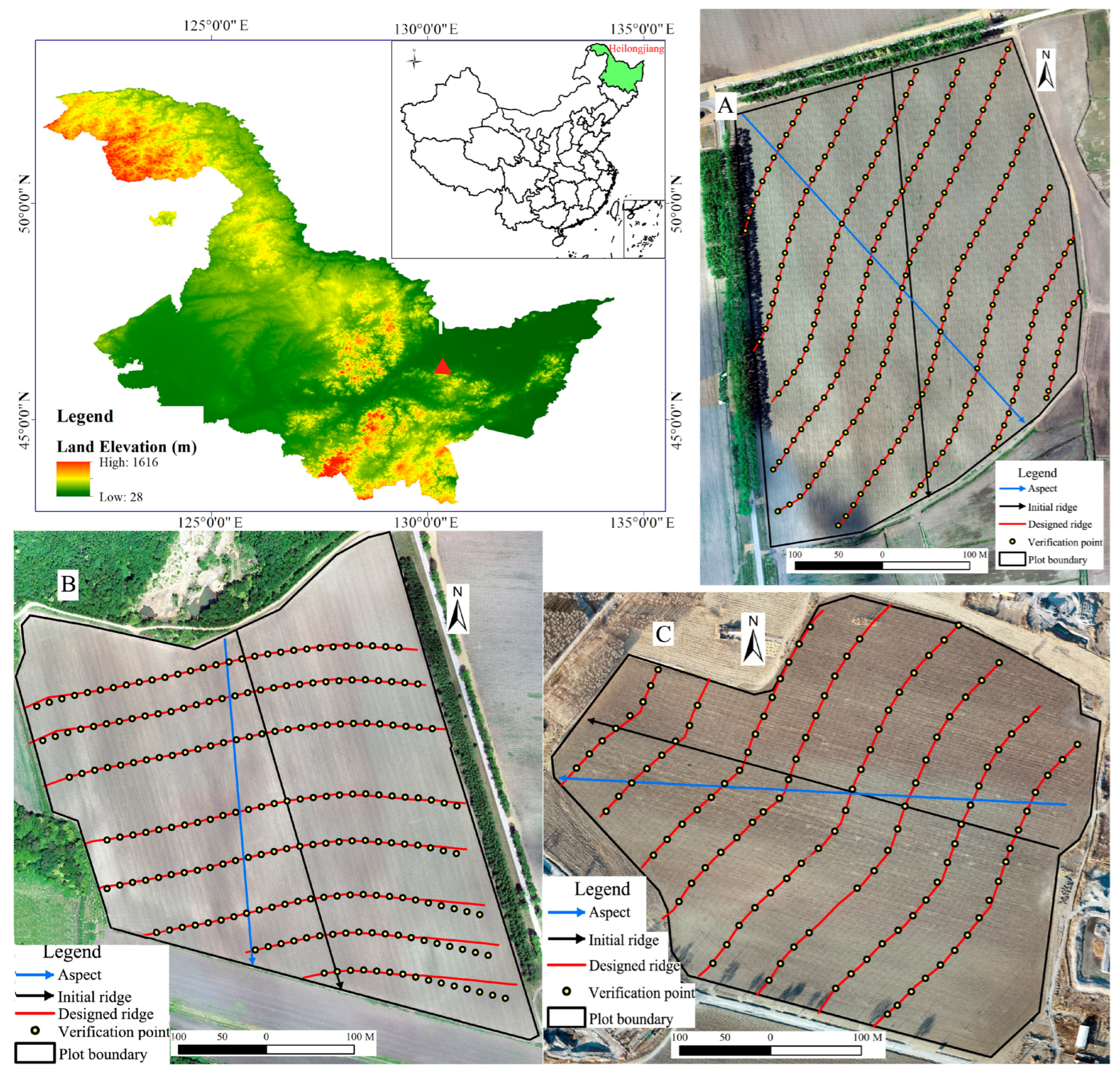
2.1. Study Area

The slope farmland plots for contour ridging are located at Beixing Farm and Shuangyashan Farm in the northeastern part of the Sanjiang Plain in Heilongjiang Province, China (Figure 1). These three plots are identified as A, B, and C, with geographic coordinates at E 131.466 and N 46.198, E 131.419 and N 46.153, and E 131.388 and N 46.588, respectively. Their areas are 17.3, 19.8, and 20.2 hectares, with natural slope gradients of 2.5°, 3.0°, and 3.0°, respectively (Table 1). All three plots were initially under traditional downslope ridging. Aspect and initial ridge orientations of these three plots were as follows: Plot A had a southeast-facing slope with ridges higher in the north and lower in the south, Plot B had a south-facing slope with ridges higher in the north and lower in the south, and Plot C had a west-facing slope with ridges higher in the east and lower in the west. Therefore, all these slope farmlands met the natural slope gradient and ridge orientation requirements for contour ridging in the black soil region. The slope gradient along the downslope ridge for these three slope farmlands was 1.3°, 2.6°, and 2.7°, respectively.

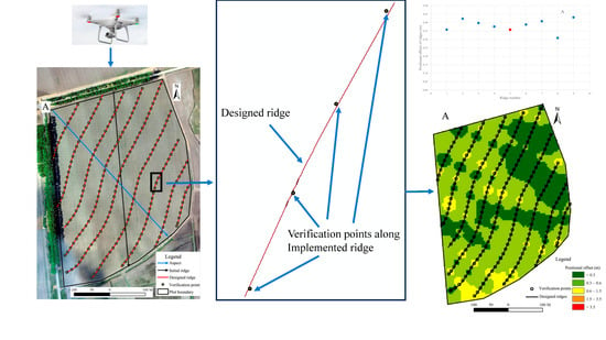
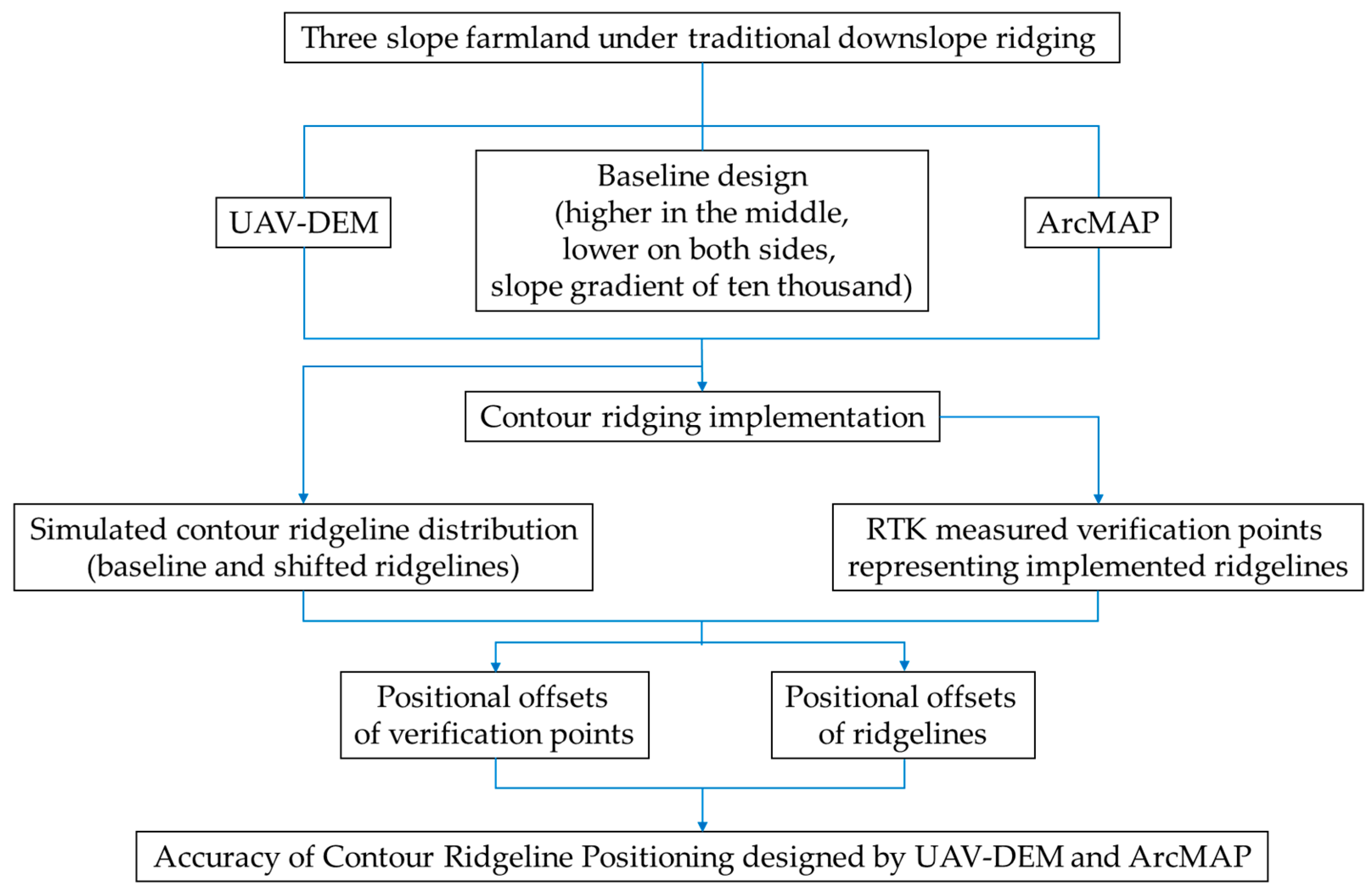
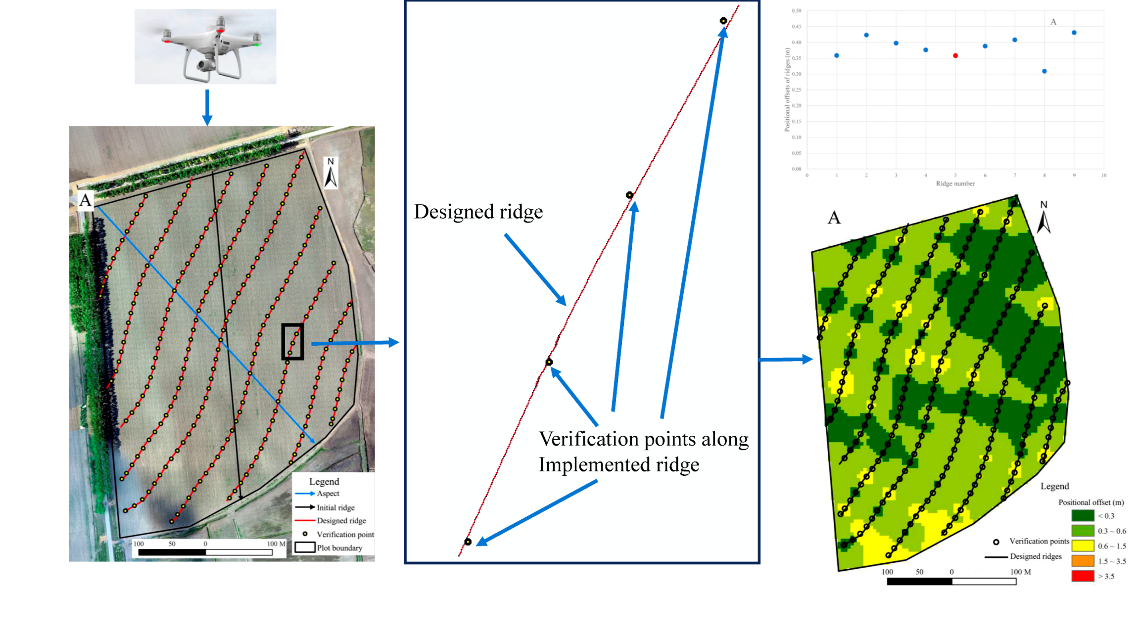
2.2. Design and Implementation of Contour Ridging

Considering the benefits of rapid drainage of spring meltwater to raise the surface temperature and facilitate seed germination in the region, this study opted to design contour ridges with appropriate gradients along the ridge direction. Previous studies have shown that black soil with gentle slope tops yields higher production [30]. Consequently, the baseline design adopted a configuration that was higher in the middle and lower on the sides. This design shortened the length of the concentrated flow slopes and potentially increased yield. Combining the “Code for design of water and soil conservation engineering (GB 51018-2014 [31])” with the field conditions of soil erosion in this region, the study ultimately established a baseline configuration that was higher in the middle, lower on both sides, with a slope gradient of ten thousandths along ridge direction.
After harvest in November 2022, the DJI Phantom 4 RTK drone was utilized to obtain DEM with a resolution of 3 cm for these three slope farmlands (Figure 2). Once this DEM was imported into ArcMap, one of the two intersection points where the longest contour line crossed the plot’s boundary was randomly selected as the initial point. From the initial point, XYZ coordinates of ground points were obtained at 15 m intervals, continuing until reaching the other side of the slope farmland. The coordinates of these ground points were calculated based on the elevation values from the DEM and the elevation changes along the baseline (higher in the middle, lower on both sides, with a slope gradient of ten thousandths along the ridge direction), as well as point interval of 15 m. After the baseline design was completed, vector data of points along the baseline were imported into the CHCNAV RTK notebook. Utilizing the CORS network RTK mode, flags were placed every 15 m on the ground within farmland based on the coordinates of ground points. The line formed by these flags represented the baseline. Ridging machinery with a navigation system was applied to travel along the baseline to record its trajectory. Then, the navigation system guided the ridging machine to perform parallel ridging. The ridging machine had three rows, each 50 inches wide. The Trimble CFX-750 model navigation device was used for Plots A and B, while the Qianyun QY210 model navigation device was employed for Plot C.

2.3. Data Collection

Within each slope farmland, nine contour ridges, including the baseline (eight ridges for plot 3), were selected as verification lines for verifying the accuracy of the contour ridgeline positions. These ridgelines were evenly distributed across the corresponding slope farmland area. Along each ridgeline, a point was selected every 15 m as a verification point. The verification point’s coordinates (XYZ) were measured using the CHCNAV RTK in a fixed solution state (10 mm + 1 ppm horizontally and 20 mm + 1 ppm vertically). During measurement, the bottom of the RTK pole was placed in the middle of the furrow on the ground and kept level. Since the RTK pole might penetrate the topsoil under its weight, ensuring that the bottom of the RTK pole remained on the surface of the topsoil was important, thereby guaranteeing the elevation measurements represent the surface elevation. The designed ridgelines and the verification points were based on the WGS84 planar coordinate system. In total, 223 verification points from nine contour ridges on plot A, 204 verification points from nine ridges on plot B, and 118 verification points from eight ridges on plot C were measured.

2.4. Data Analysis

The difference between the implemented ridgelines’ positions and the designed ridgelines’ positions reflects the accuracy of designing contour ridging using ArcMap software. The XYZ coordinates measured along the ridgelines represent the field positions of the implemented ridges, and the designed ridgelines’ position could be obtained by replicating and shifting the designed baseline to the measured ridgelines in ArcMap. Taking Plot A as an example, the designed baseline in ArcMap was copied and shifted to overlay the measured ridgelines. A total of eight designed contour ridgelines were replicated and moved. Including the baseline, this study will assess the differences between the designed and field positions of nine ridgelines in plot A.
The slope gradient between adjacent verification points on the same ridge line was calculated based on their elevation change and interval (about 15 m). The slope gradient along each contour ridgeline was calculated by averaging the slope gradients of all verification points on that ridge.
Using the ‘Near’ function in the ArcMap software, the distance from each verification point along the implemented contour ridge to the corresponding position on the designed ridge was calculated. This distance was considered as the positional offset value of the corresponding verification point. The average offset value of all verification points on each ridge was then calculated, representing the average positional offset for that ridge.
The frequency distribution of these offset values was analyzed, and spatial distribution maps of the offsets were generated to examine their spatial characteristics. Besides, the study quantified the average offset for individual contour ridges and analyzed the spatial variation characteristics of these offset values.

3. Results

3.1. Slope Gradient along Contour Ridgelines

Results showed that there were no significant differences in the average slope gradient along contour ridgelines among the three slope farmlands, which were 0.54° ± 0.08°, 0.62° ± 0.07°, and 0.54° ± 0.06°, respectively (Table 2). Although contour ridging could only design the gradient along the baseline, the measured slope gradient along implemented ridges was marginally different from the designed value (ten thousandths, approximately 0.57°). This indicates that the designed slope gradient along the baseline could approximately represent the average slope gradient along other contour ridges. On the other hand, although the average value of the measured slope gradients was closely aligned with the designed value, there was still some variation between the measured and designed slope gradients. Across all ridgelines in the three farmlands, the minimum measured slope gradient was 0.4°, and the maximum was 0.8°. This range indicates that the measured slope gradient along contour ridgelines fell within a 40% range above and below the design values of 0.57°.

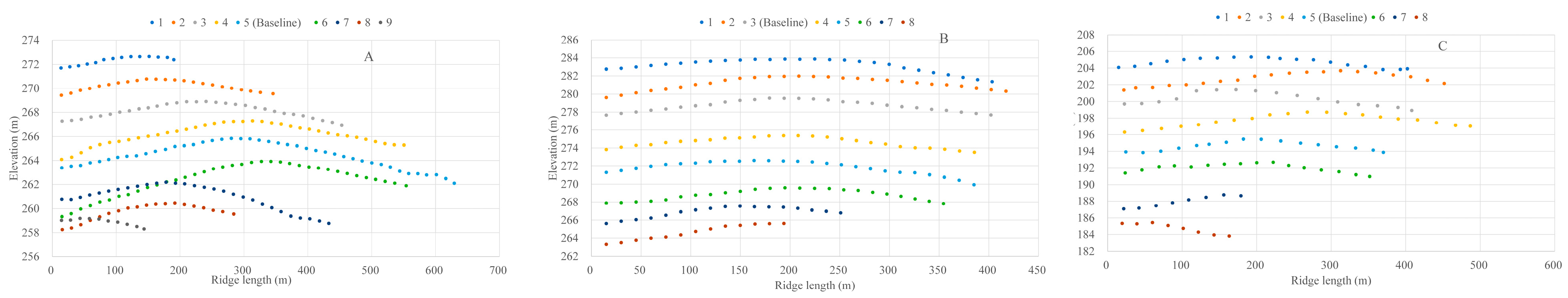
3.2. Elevation Variation along Contour Ridgelines

Based on the elevation values of verification points along individual ridges, elevation changes along the ridges in the three farmlands were created (Figure 3). Most contour ridges were higher in the middle and lower on the sides, consistent with the baseline design (Ridge 5 in plot A, Ridge 3 in plot B, and Ridge 4 in plot C). Some measured ridges exhibited a trend of being higher on one side, such as Ridge 8 in Plot B and Ridge 8 in Plot C. However, the elevation changes along the implemented ridgelines did not completely match those of the designed baseline. For some implemented ridgelines, the highest elevation points were not located precisely in the middle of the ridgeline, such as ridges 6 and 7 in plot A, ridge 7 in plot B, and ridge 2 in plot C.

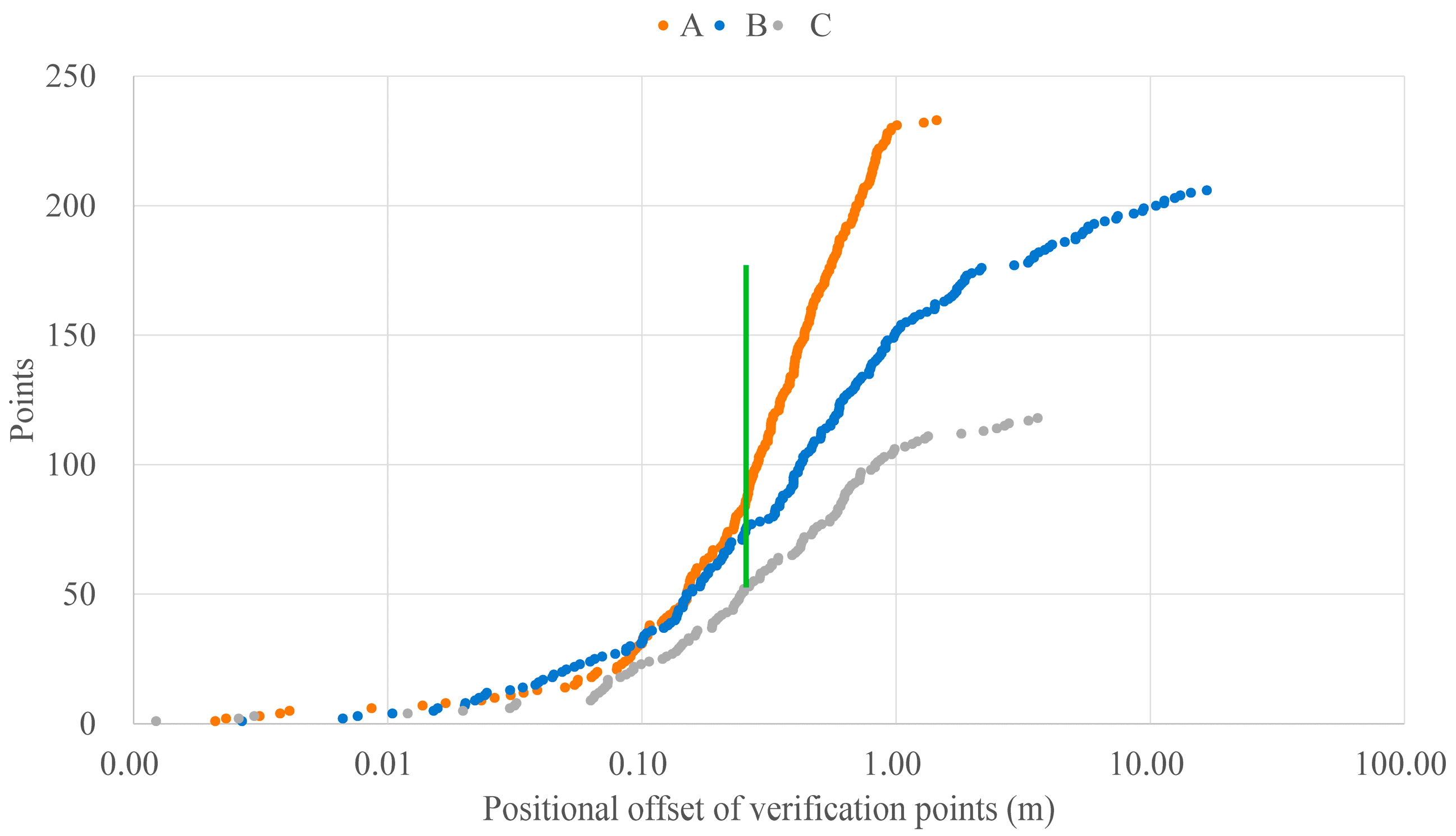
3.3. Statistical Analysis of Verification Point Positional Offsets

The average offset values of the verification points for the three farmlands were 0.38 ± 0.03, 1.11 ± 0.38, and 0.52 ± 0.12 m, respectively (Table 3), with plot B significantly larger than plots A and C. There was no significant difference between plots A and C. Given that the maximum offset value of verification points in plot B (16.69 m) was substantially larger than those in plot A (1.45 m) and plot C (3.61 m), it implied that some verification points in plot B could exhibit significantly larger offset values. Therefore, the median value could be more appropriate for describing the distribution of offset data. Compared to the average values, the median offsets of verification points in the three plots were relatively similar at 0.32, 0.43, and 0.31 m, respectively. This indicated that 50% of the verification points in each plot had offsets less than 0.32, 0.43, and 0.31 m.
Since the design and implementation processes of contour ridging were consistent across the three plots, further investigation was required into why the offset values for verification points in plot B were significantly larger than those values in plots A and C. Considering that the maximum offset value in plot B (16.69 m) substantially surpassed the range of offset values in plots A and C (1.45 and 3.61 m), a new dataset was created by extracting verification points from plot B with offset values less than the maximum value of 3.61 m observed in plot C. This revised dataset, named B-Corrected, retained 180 points out of the original 204 points. Statistical analysis revealed significant differences in the offset data of plot B before and after the correction. After the correction, the offset values of the verification points in plot B did not significantly differ from those in plots A and C.
Due to the significantly larger maximum (16.69 m) and average (1.11 m) offset values of verification points in plot B compared to plots A and C, a frequency distribution with a logarithmic x-axis was utilized to examine the data distribution of substantial offset values (Figure 4). Most verification points had offset values less than 0.4 m (indicated by the green vertical line), aligning with the median values in Table 3. In plot B, the offset values of verification points displayed a long-tail distribution. The number of points within the 0 to 2.2 m offset range was 176, accounting for 87% of the total, while only 30 points fell in the 2.2 to 16.7 m offset range, representing 13%. This pattern indicated that a small proportion of the verification points in plot B had substantial offset values, significantly skewing the overall distribution.

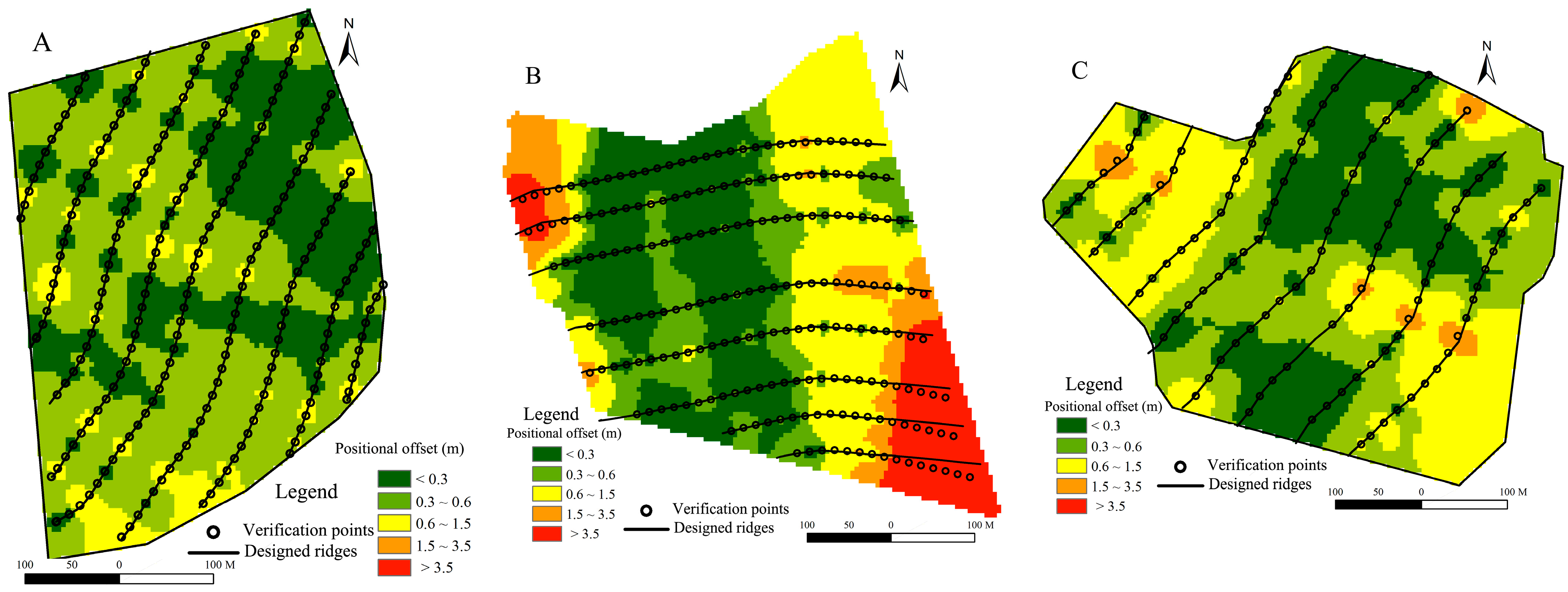
3.4. Spatial Distribution of Verification Point Positional Offsets

For each of the three farmlands, the offset values of the verification points were interpolated using the inverse distance method within their respective areas. Since the median offset values for plots A and C were slightly larger than 0.3 m and the average values were less than 0.6 m, and considering the presence of significantly larger offset points in plot B, a five-tier color grading was established for depicting offset magnitudes (Figure 5): the minimum median offset value among all three plots (0.3 m), the more considerable average value between plots A and C (0.6 m), the maximum value in plot A (1.5 m), the maximum value in plot C (3.6 m), and the maximum value in plot B (16.7 m). In this scheme, the deeper the color, the larger the offset value. Most of the verification point offsets for these three plots were under 1.5 m. For plot A, verification point offsets between 0 and 0.3 m, 0.3 and 0.6 m, 0.6 and 1.5 m occupied 25%, 64%, and 11% of total points, respectively. Such values of plot C were 32%, 31%, and 29%, respectively, and the left 9% were between 1.5 and 3.5 m. For plot B, around one-third of the total points’ offsets were larger than 1.5 m.
These interpolated values were then overlaid with the designed ridgelines to analyze the spatial distribution pattern of the verification points’ offset values. Figure 5 also demonstrates a spatial distribution pattern for verification points with larger offsets. In plot B, the points with the largest offsets (indicated by the darkest color) were all located at the edges of the plot (Figure 5B), meaning these points had larger positional offsets than the maximum values found in plots A and C (3.6 m). Combining this with Section 2.3, it was evident that the presence of these extreme outlier verification points was why the positional offsets of verification points in plot B were significantly larger than those in plots A and C. In the three plots, areas with the same color were continuously spread, indicating that verification points with similar offsets were predominantly clustered. At the same time, a small number of patchy areas were dispersed in a dotted pattern. By comparing the color of these spotty patches with the surrounding areas, it was evident that these patches, typically surrounded by lighter-colored areas, represent verification points with larger offsets than their neighboring regions. The correlation of the larger offset patches with the corresponding ridgelines indicated that these dispersed dot-like patches with larger offsets were typically located at the turns of the contour ridgelines. On the other hand, within each farmland, areas with larger offsets (indicated by darker colors) were predominantly along the edges of the respective regions. This suggests that verification points with larger offsets were also more commonly found at the edges of these regions. Given that the designed baseline was situated in the middle of the slope farmland, the offset of verification points tended to decrease as they approached the center of the farmland or the designed baseline.

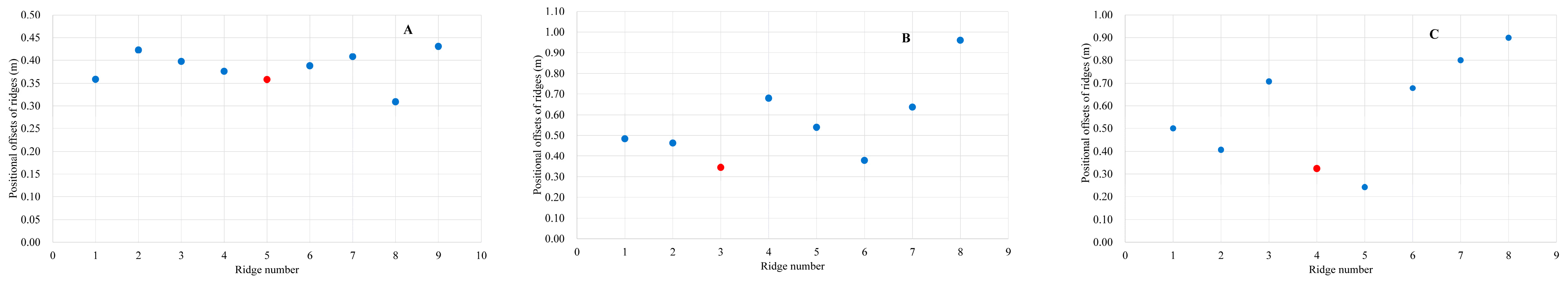
3.5. Positional Offsets of Ridgelines

The average offset value for each ridgeline was calculated by averaging the offset values of verification points along the ridgeline. This average value was used to represent the positional offset of that ridgeline. A dot distribution chart of ridgeline positional offsets was created, following the spatial arrangement of the implemented ridgelines with the baseline in the middle and successive ridgelines extending on either side. Figure 6 demonstrates a distribution trend of ridgeline offsets being lower in the middle and higher on both sides, indicating that the positional offset of the ridgelines increases with distance from the baseline. Several ridgelines in plot C, including ridges 6, 7, and 8, exhibited significant positional offsets. However, the short length of these ridgelines did not significantly affect the average ridgeline offset. Moreover, there was a notable variation in ridgeline positional offsets across different plots. For instance, ridgeline offsets in plot A ranged from 0.3 to 0.5 m, while plot C ranged from 0.2 to 1.0 m.

4. Discussion

4.1. Soil and Water Conservation Effects of Contour Ridging

Contour ridging primarily mitigates soil erosion by reducing the gradient along the ridgelines. Therefore, the percentage reduction in slope gradient along the ridgeline is a crucial indicator of the effectiveness of contour ridging implementation [32]. In this study, the slope gradient along ridges of the three slope farmland decreased from 1.3°, 2.6°, and 2.7° to 0.54°, 0.62°, and 0.54° respectively. This represents a 58%, 76%, and 80% decrease in slope gradient along ridgeline within these three farmlands (see Table 4), which indicates that the soil conservation benefits increased by at least 50% after implementing contour ridging. As runoff in slope farmland flows along the ridges’ direction, the slope gradient reduction due to contour ridging significantly lowers the surface runoff velocity. The decrease in runoff velocity reduces sediment’s carrying and transporting capacity by runoff, thus diminishing topsoil erosion, increasing sediment deposition, and mitigating the spatial heterogeneity of nutrients caused by nutrient loss with sediment-laden runoff [33]. The reduction in slope gradient along the ridge also implies that surface runoff would be difficult to discharge, which may cause waterlogging within slope farmland. Given that soybeans are susceptible to waterlogging [34], contour ridging might be more appropriate for corn. Additionally, for soils with low infiltration rates, such as vertosols, increasing the slope gradient along ridge to enhance the capacity for surface runoff discharge is advised; for soils with high infiltration rates, such as sandy soils, decrease the ridge orientation slope to reduce the capacity for surface runoff discharge could be appropriate.
Empirical or process-based soil erosion estimation models [35], such as RUSLE (Revised Universal Soil Loss Equation) and WEPP (Water Erosion Prediction Project), are the primary methods for assessing the benefits of soil conservation measures at slope farmland. These models can evaluate the soil conservation benefits of contour ridging by modifying the gradient along ridges. Since this paper’s primary focus was on the ridgelines’ positional offsets, direct measurements or model calculations of soil loss intensity were not applied. This study utilized existing research on soil erosion in the Northeast Black Soil Region’s slope farmland to estimate the intensity of soil erosion after contour ridging in these plots. Dai et al.’s [36] results from runoff plots in the black soil region showed that soil erosion on downslope ridge farmland was 1094 t/km2·a. Zhu et al.’s [37] soil loss model simulations for slope farmland indicated an average soil erosion of 709 t/km2·a. Both studies reported soil loss intensities exceeding 700 t/km2·a for slope farmland. Considering the soil conservation factor for contour ridging of 0.2 in this study, it could be inferred that after implementing contour ridging, the soil erosion intensity on slope farmland could be approximately 150 t/km2·a. The current national standard for soil loss tolerance (T) in the black soil region of Northeast China was empirically determined at 200 t/km2·a [38], and the result from 21 black soil types in this region indicated a range of soil loss tolerance from 68 t/km2·a to 358 t/km2·a. This variability highlighted the diverse soil erosion characteristics within the region. Therefore, it could be inferred that the soil erosion intensity resulting from contour ridging in this study was close to the permissible soil loss range for the region. Investigation of 290 observations of crop yields from topsoil removal experiments worldwide demonstrated that a horizon depth of 25 cm may be a threshold for sustainable soil productivity in eroded soils [39]. Given that the average depth of black topsoil is less than 30 cm due to serious soil erosion [40], contour ridging could be crucial for sustainable agriculture in Northeast China because it could ensure agricultural yield while reducing soil erosion intensity to soil loss tolerance.

4.2. Positional Offset of Contour Ridging Ridgelines

Despite the reduced slope gradient along ridgeline demonstrated that contour ridging effectively mitigated soil erosion in slope farmland, a discrepancy existed between the implemented and designed positions of the ridgelines. Results indicated that the three farmlands’ median positional offset of verification points was 0.3 to 0.4 m, approximately one-third of one ridge width. Verification points with larger offsets were primarily distributed along the edges of slope farmland and at the turning points of the ridgelines. The positioning of baseline markers and the navigation-guided ridging by the machinery were two distinct phases in the implementation of contour ridging. Consequently, the positional offsets of the verification points could be the result of these two processes. Due to most of the navigation software on sale in northeast China currently not supporting the import function for designed ridgelines, manual baseline setup methods were needed. The baseline markers were positioned using CORS RTK in a fixed solution state, ensuring a positioning error of less than 2 cm. The navigation devices in the ridging machinery utilized GPS or BeiDou satellite signals, typically achieving accuracy with an error of less than 5 cm [41]. After recording the baseline information by traveling along the baseline points, the ridging machinery performed ridging parallel to the baseline, relying on navigation guidance. Various technical factors, including navigation positioning, path planning, and motion control, influenced the accuracy of the ridging trajectory of machinery [42,43]. Although the navigation device calculates and guides the movement trajectory of the ridging machinery based on the baseline position and ridging width, the long-distance work could lead to positional error accumulation [44]. This error accumulation made it challenging to maintain accuracy over extended periods. Thus, relative to the baseline marker setup, the navigation process during ridging was likely the leading cause for the increasing offset observed with larger distances from the baseline.
Currently, many agricultural machinery navigation devices in China are retrofitted systems, predominantly using electric power steering, which has inherent steering slack and is less precise. If the curvature of the ridgeline was too sharp, it could lead to a delay in steering control relative to the navigational position [45], causing the path of the agricultural machinery to diverge from the navigational guidance. Therefore, during the phases of baseline design and the placement of marker points, it was essential to ensure that the curvature of turns was kept within a specific limit and as smooth as possible.

4.3. Impact on the Baseline Setup of Contour Ridging

The implementation process of contour ridging includes designing the baseline, setting up the baseline, and ridging guided by navigation. Importing the baseline coordinate data into the layout equipment was needed during the baseline setup. Then, marker points were placed on the ground at certain intervals, and the line connecting these points represented the position of the baseline. The layout equipment for setting up the baseline is influenced by factors such as the equipment’s portability, ease of use, and precision. Typically, the higher the accuracy of the layout equipment, the lower its portability and ease of use. Additionally, the acquisition cost and expertise required for operating the equipment tend to increase with higher precision. Traditional surveying equipment like total stations or level instruments could offer millimeter-level accuracy in layout precision, but their setup and measurement processes are complex and time-consuming. Satellite-based differential GPS surveying devices, such as base station-dependent RTK and network-based CORS RTK, can achieve centimeter-level accuracy. However, using these devices generally involves tasks like setting coordinate zones and converting formats, requiring a certain level of professional knowledge from the operators. With the development of the BeiDou Satellite Navigation System [46], it now offers users dynamic decimeter-level high-precision positioning capabilities. Devices capable of sub-meter and decimeter-level positioning also feature good portability and ease of use, like BeiDou Probe. In this study, CHCNAV RTK was utilized in connection with Qianxun’s FindCM high-precision positioning service, which offered centimeter-level positioning accuracy. However, the positional offset of the baseline after implementation still reached a decimeter level, ranging between 20 to 30 cm. If the offset of verification points set using decimeter-level positioning devices were similar to the offsets observed in this study, it would significantly reduce the equipment cost and enhance the efficiency of marker placement. Consequently, future research could figure out the offset values associated with baseline setup using decimeter-level positioning devices.

4.4. Recommendations for Navigation-Based Ridging

The agricultural machinery navigation system computes the operational routes within defined areas based on the baseline position information and ridging width recorded by the system [47], thereby guiding the movement of the machinery. The accuracy of navigation devices and the operator’s driving habits influence the machinery’s movement accuracy [48]. Although most navigation devices in the agricultural sector have a precision of ±2.5 cm along straight lines, the field navigation accuracy may exceed this designed value because the machinery follows a curved path during contour ridging. Communicating with the agricultural machinery operators revealed that a few navigation devices with stable signals could maintain stability within 2.5 cm. However, the accuracy of most navigation devices can reach up to 5 cm, especially with large turning angles on the ridgelines, which could lead to overlapping between two adjacent ridgelines. Reducing the driving speed appropriately could often improve movement accuracy when ridgeline turning angles were large, thereby reducing the offset at turning points. Additionally, due to accumulative errors, gaps or overlaps between adjacent ridgelines often emerged after completing the ridging of several dozen lines. In such cases, the most recently completed ridgeline could be used as a new baseline and re-entered into the navigation system. Then, using this ridgeline as the baseline, navigational ridging could be conducted for the remaining areas yet to be ridged. Although re-establishing a baseline and then ridging cannot eliminate the error, it can reduce the occurrence of gaps or overlaps between adjacent ridgelines.

4.5. Implications for Future Works

The spatial distribution of the baseline, as well as simulated ridgelines, were obtained using ArcGIS and high-precision DEM in this research. Indeed, the spatial distribution of slope gradient along contour ridgelines could also be obtained based on the spatial distribution of these simulated ridgelines. The research revealed that the positional offsets of ridgelines varied within the slope farmland. Consequently, discrepancies between the measured and simulated values of slope gradient along contour ridgelines might exist and exhibit spatial heterogeneity. The effect of spatial variability of slope gradient along contour ridgelines on the redistribution of soil moisture, nutrients, and sediments needs to be further demonstrated. Besides, investigating the impact of the discrepancies between the measured and simulated values of slope gradient along contour ridgelines on the model simulations of the aforementioned processes is worth exploring.

5. Conclusions

(1)
Designing contour ridgelines using ArcMap can effectively estimate the effect of implemented contour ridging. The average measured slope gradient along ridgelines (0.5~0.6°) closely matches the designed value (0.6°), representing a 50% to 70% reduction compared to the original slope gradient along traditional downslope ridging. Regarding elevation changes along the ridgelines, most of the measured ridgelines were consistent with the designed baseline, being higher in the middle and lower on both sides, which shortened the length of overland flow on the slope;
(2)
At the field scale, the average positional offset between the contour ridgelines designed using ArcMap and the implemented ridgelines is less than a single ridge width (1.3 m wide). The median offset is only one-third of a single ridge width. Additionally, the error contributed by the movement of the ridging machinery may be larger than the error of the baseline setup;
(3)
The larger the distance from the baseline, the larger the positional offset between the measured and designed ridgelines. Besides, the positional offset between the measured and designed ridgelines is notably larger at the turning points. Therefore, the turns should be made as smooth as possible when designing ridgelines. During ridging, reducing the speed at these turns is recommended to minimize errors and maintain the accuracy of the ridging path.

Author Contributions

H.L. and C.S. designed the research; W.Z. and J.W. processed and analyzed the data; J.W. and X.G. collected the data; H.L. wrote the paper. All authors have read and agreed to the published version of the manuscript.

Funding

This study was founded by the Strategic Priority Research Program of the Chinese Academy of Sciences (XDA28100403); Doctoral Startup Foundation of Liaocheng University (318052031).

Institutional Review Board Statement

Not applicable.

Informed Consent Statement

Not applicable.

Data Availability Statement

Summarized data are presented and available in this manuscript, and the rest of the data used and/or analyzed are available from the corresponding author on reasonable request.

Conflicts of Interest

Author Hao Li was employed by the company Liaocheng Innovative High Resolution Data Technology Co. The remaining authors declare that the research was conducted in the absence of any commercial or financial relationships that could be construed as a potential conflict of interest.

References

  1. Wang, H.; Zhang, C.; Yao, X.; Yun, W.; Ma, J.; Gao, L.; Li, P. Scenario simulation of the tradeoff between ecological land and farmland in black soil region of Northeast China. Land Use Policy 2022, 114, 105991. [Google Scholar] [CrossRef]
  2. Gong, H.; Meng, D.; Li, X.; Zhu, F. Soil degradation and food security coupled with global climate change in northeastern China. Chin. Geogr. Sci. 2013, 23, 562–573. [Google Scholar] [CrossRef]
  3. Zhang, P. Revitalizing old industrial base of Northeast China: Process, policy and challenge. Chin. Geogr. Sci. 2008, 18, 109–118. [Google Scholar] [CrossRef]
  4. Wang, Z.; Liu, B.; Wang, X.; Gao, X.; Liu, G. Erosion effect on the productivity of black soil in Northeast China. Sci. China Ser. D Earth Sci. 2009, 52, 1005–1021. [Google Scholar] [CrossRef]
  5. Sui, Y.; Liu, X.; Jin, J.; Zhang, S.; Zhang, X.; Herbert, S.J.; Ding, G. Differentiating the early impacts of topsoil removal and soil amendments on crop performance/productivity of corn and soybean in eroded farmland of Chinese Mollisols. Field Crops Res. 2009, 111, 276–283. [Google Scholar] [CrossRef]
  6. Li, H.; Cruse, R.M.; Liu, X.; Zhang, X. Effects of topography and land use change on gully development in typical Mollisol region of Northeast China. Chin. Geogr. Sci. 2016, 26, 779–788. [Google Scholar] [CrossRef]
  7. Zhang, S.; Han, X.; Cruse, R.M.; Zhang, X.; Hu, W.; Yan, Y.; Guo, M. Morphological characteristics and influencing factors of permanent gully and its contribution to regional soil loss based on a field investigation of 393 km2 in Mollisols region of northeast China. CATENA 2022, 217, 106467. [Google Scholar] [CrossRef]
  8. Liu, X.B.; Zhang, X.Y.; Wang, Y.X.; Sui, Y.Y.; Zhang, S.L.; Herbert, S.J.; Ding, G. Soil degradation: A problem threatening the sustainable development of agriculture in Northeast China. Plant Soil Environ. 2010, 56, 87–97. [Google Scholar] [CrossRef]
  9. Fan, H.; Hou, Y.; Xu, X.; Mi, C.; Shi, H. Composite Factors during Snowmelt Erosion of Farmland in Black Soil Region of Northeast China: Temperature, Snowmelt Runoff, Thaw Depths and Contour Ridge Culture. Water 2023, 15, 2918. [Google Scholar] [CrossRef]
  10. Wang, L.; Zheng, F.; Zhang, X.J.; Wilson, G.V.; Qin, C.; He, C.; Liu, G.; Zhang, J. Discrimination of soil losses between ridge and furrow in longitudinal ridge-tillage under simulated upslope inflow and rainfall. Soil Tillage Res. 2020, 198, 104541. [Google Scholar] [CrossRef]
  11. Xin, Y.; Liu, G.; Xie, Y.; Gao, Y.; Liu, B.; Shen, B. Effects of soil conservation practices on soil losses from slope farmland in northeastern China using runoff plot data. CATENA 2019, 174, 417–424. [Google Scholar] [CrossRef]
  12. Gathagu, J.N.A.A.; Mourad, K.A.; Sang, J.J.W. Effectiveness of contour farming and filter strips on ecosystem services. Water 2018, 10, 1312. [Google Scholar] [CrossRef]
  13. Geng, R.; Yin, P.; Sharpley, A.N. A coupled model system to optimize the best management practices for nonpoint source pollution control. J. Clean. Prod. 2019, 220, 581–592. [Google Scholar] [CrossRef]
  14. Jia, L.; Zhao, W.; Zhai, R.; An, Y.; Pereira, P. Quantifying the effects of contour tillage in controlling water erosion in China: A meta-analysis. CATENA 2020, 195, 104829. [Google Scholar] [CrossRef]
  15. Saggau, P.; Kuhwald, M.; Duttmann, R. Effects of contour farming and tillage practices on soil erosion processes in a hummocky watershed. A model-based case study highlighting the role of tramline tracks. CATENA 2023, 228, 107126. [Google Scholar] [CrossRef]
  16. Wei, W.; Chen, D.; Wang, L.; Daryanto, S.; Chen, L.; Yu, Y.; Lu, Y.; Sun, G.; Feng, T. Global synthesis of the classifications, distributions, benefits and issues of terracing. Earth-Sci. Rev. 2016, 159, 388–403. [Google Scholar] [CrossRef]
  17. Morgan, R.P.C. Soil Erosion and Conservation; John Wiley & Sons: Hoboken, NJ, USA, 2009. [Google Scholar]
  18. Yu, P.; Yang, T.; Zhang, Z.; Zhou, X.; Qi, Z.; Yin, Z.; Li, A. Soil and water conservation effects of different tillage measures on phaeozems sloping farmland in northeast China. Land Degrad. Dev. 2024, 35, 1716–1733. [Google Scholar] [CrossRef]
  19. Farahani, S.; Fard, F.; Asoodar, M. Effects of contour farming on runoff and soil erosion reduction: A review study. Elixir Agric. 2016, 101, 44089–44093. [Google Scholar]
  20. Laflen, J.M.; Highfill, R.E.; Amemiya, M.; Mutchler, C.K. Structures and Methods for Controlling Water Erosion. In Soil Erosion and Crop Productivity; John Wiley & Sons: Hoboken, NJ, USA, 1985; pp. 431–442. [Google Scholar]
  21. Chen, X.; Liang, Z.; Zhang, Z.; Zhang, L. Effects of Soil and Water Conservation Measures on Runoff and Sediment Yield in Red Soil Slope Farmland under Natural Rainfall. Sustainability 2020, 12, 3417. [Google Scholar] [CrossRef]
  22. Scholand, D.; Schmalz, B. Deriving the Main Cultivation Direction from Open Remote Sensing Data to Determine the Support Practice Measure Contouring. Land 2021, 10, 1279. [Google Scholar] [CrossRef]
  23. Thompson, A.; Sudduth, K. Terracing and Contour Farming. In Precision Conservation: Geospatial Techniques for Agricultural and Natural Resources Conservation; John Wiley & Sons: Hoboken, NJ, USA, 2017; pp. 151–163. [Google Scholar]
  24. Guo, W.J.; Maas, S. Terrace Layout Design Utilizing Geographic Information System and Automated Guidance System. Appl. Eng. Agric. 2012, 28, 31–38. [Google Scholar] [CrossRef]
  25. Guo, W. Application of Geographic Information System and Automated Guidance System in Optimizing Contour and Terrace Farming. Agriculture 2018, 8, 142. [Google Scholar] [CrossRef]
  26. Pineux, N.; Lisein, J.; Swerts, G.; Bielders, C.L.; Lejeune, P.; Colinet, G.; Degré, A. Can DEM time series produced by UAV be used to quantify diffuse erosion in an agricultural watershed? Geomorphology 2017, 280, 122–136. [Google Scholar] [CrossRef]
  27. Kou, P.; Xu, Q.; Yunus, A.P.; Ju, Y.; Guo, C.; Wang, C.; Zhao, K. Multi-temporal UAV data for assessing rapid rill erosion in typical gully heads on the largest tableland of the Loess Plateau, China. Bull. Eng. Geol. Environ. 2020, 79, 1861–1877. [Google Scholar] [CrossRef]
  28. Wang, R.; Sun, H.; Yang, J.; Zhang, S.; Fu, H.; Wang, N.; Liu, Q. Quantitative Evaluation of Gully Erosion Using Multitemporal UAV Data in the Southern Black Soil Region of Northeast China: A Case Study. Remote Sens. 2022, 14, 1479. [Google Scholar] [CrossRef]
  29. Shi, Z.H.; Cai, C.F.; Ding, S.W.; Wang, T.W.; Chow, T.L. Soil conservation planning at the small watershed level using RUSLE with GIS: A case study in the Three Gorge Area of China. CATENA 2004, 55, 33–48. [Google Scholar] [CrossRef]
  30. Zhang, S.; Jiang, L.; Liu, X.; Zhang, X.; Fu, S.; Dai, L. Soil nutrient variance by slope position in a Mollisol farmland area of Northeast China. Chin. Geogr. Sci. 2016, 26, 508–517. [Google Scholar] [CrossRef]
  31. GB 51018-2014; Code for Design of Soil and Water Conservation Engineering. Ministry of Housing and Urban Rural Development of the People’s Republic of China: Beijing, China, 2014.
  32. Panagos, P.; Borrelli, P.; Meusburger, K.; van der Zanden, E.H.; Poesen, J.; Alewell, C. Modelling the effect of support practices (P-factor) on the reduction of soil erosion by water at European scale. Environ. Sci. Policy 2015, 51, 23–34. [Google Scholar] [CrossRef]
  33. Ricci, G.F.; Jeong, J.; De Girolamo, A.M.; Gentile, F. Effectiveness and feasibility of different management practices to reduce soil erosion in an agricultural watershed. Land Use Policy 2020, 90, 104306. [Google Scholar] [CrossRef]
  34. Li, S.; Xie, Y.; Liu, G.; Wang, J.; Lin, H.; Xin, Y.; Zhai, J. Water Use Efficiency of Soybean under Water Stress in Different Eroded Soils. Water 2020, 12, 373. [Google Scholar] [CrossRef]
  35. Tiwari, A.K.; Risse, L.M.; Nearing, M.A. Evaluation of WEPP and its comparison with USLE and RUSLE. Trans. ASAE 2000, 43, 1129–1135. [Google Scholar] [CrossRef]
  36. Dai, T.; Wang, L.; Li, T.; Qiu, P.; Wang, J. Study on the Characteristics of Soil Erosion in the Black Soil Area of Northeast China under Natural Rainfall Conditions: The Case of Sunjiagou Small Watershed. Sustainability 2022, 14, 8284. [Google Scholar] [CrossRef]
  37. Zhu, Y.; Li, W.; Wang, D.; Wu, Z.; Shang, P. Spatial Pattern of Soil Erosion in Relation to Land Use Change in a Rolling Hilly Region of Northeast China. Land 2022, 11, 1253. [Google Scholar] [CrossRef]
  38. Duan, X.; Xie, Y.; Liu, B.; Liu, G.; Feng, Y.; Gao, X. Soil loss tolerance in the black soil region of Northeast China. J. Geogr. Sci. 2012, 22, 737–751. [Google Scholar] [CrossRef]
  39. Zhang, L.; Huang, Y.; Rong, L.; Duan, X.; Zhang, R.; Li, Y.; Guan, J. Effect of soil erosion depth on crop yield based on topsoil removal method: A meta-analysis. Agron. Sustain. Dev. 2021, 41, 63. [Google Scholar] [CrossRef]
  40. Liu, L.; Zhang, K.; Zhang, Z.; Qiu, Q. Identifying soil redistribution patterns by magnetic susceptibility on the black soil farmland in Northeast China. CATENA 2015, 129, 103–111. [Google Scholar] [CrossRef]
  41. Drenjanac, D.; Tomic, S.; Agüera, J.; Perez-Ruiz, M. Wi-Fi and Satellite-Based Location Techniques for Intelligent Agricultural Machinery Controlled by a Human Operator. Sensors 2014, 14, 19767–19784. [Google Scholar] [CrossRef]
  42. Mousazadeh, H. A technical review on navigation systems of agricultural autonomous off-road vehicles. J. Terramech. 2013, 50, 211–232. [Google Scholar] [CrossRef]
  43. Shalal, N.; Low, T.; McCarthy, C.; Hancock, N.H. A Review of autonomous navigation systems in agricultural environments. In Proceedings of the SEAg 2013: Innovative Agricultural Technologies for a Sustainable Future, Barton, Australia, 22–25 September 2013. [Google Scholar]
  44. Qiangwen, F.; Liu, Y.; Liu, Z.; Li, S.; Guan, B. High-accuracy SINS/LDV Integration for Long-distance Land Navigation. IEEE/ASME Trans. Mechatron. 2018, 23, 2952–2962. [Google Scholar]
  45. Corno, M.; Panzani, G.; Roselli, F.; Giorelli, M.; Azzolini, D.; Savaresi, S. An LPV Approach to Autonomous Vehicle Path Tracking in the Presence of Steering Actuation Nonlinearities. IEEE Trans. Control Syst. Technol. 2020, 29, 1766–1774. [Google Scholar] [CrossRef]
  46. Li, R.; Zheng, S.; Wang, E.; Chen, J.; Feng, S.; Wang, D.; Dai, L. Advances in BeiDou Navigation Satellite System (BDS) and satellite navigation augmentation technologies. Satell. Navig. 2020, 1, 12. [Google Scholar] [CrossRef]
  47. Yun, C.; Kim, H.-J.; Jeon, C.-W.; Gang, M.; Lee, W.S.; Han, J.G. Stereovision-based ridge-furrow detection and tracking for auto-guided cultivator. Comput. Electron. Agric. 2021, 191, 106490. [Google Scholar] [CrossRef]
  48. Radocaj, D.; Plaščak, I.; Heffer, G.; Jurišić, M. A Low-Cost Global Navigation Satellite System Positioning Accuracy Assessment Method for Agricultural Machinery. Appl. Sci. 2022, 12, 693. [Google Scholar] [CrossRef]
Figure 1. Location of study area ((A,B) are located at Beixing Farm, and (C) is located at Shuangyashan farm).
Sustainability 16 03106 g001
Figure 2. Flowchart of contour ridging design and positional accuracy evaluation.
Sustainability 16 03106 g002
Figure 3. Elevation variation along contour ridges of three farmlands ((A), plot A, (B), plot B, (C), plot C; the ridge line numbers correspond to the ridgelines from south to north in Figure 1. The ridgeline numbered as 1st in plot B in Figure 3 is the southernmost ridge line in plot B in Figure 1).
Sustainability 16 03106 g003
Figure 4. Frequency distribution of positional offsets of verification points (A, plot A; B, plot B, C, plot C. Green line showed 0.4 m that most verification points had offset values less than this value).
Sustainability 16 03106 g004
Figure 5. Spatial distribution of positional offsets of verification points ((A), plot A; (B), plot B, (C), plot C).
Sustainability 16 03106 g005
Figure 6. The positional offset between implemented and designed ridgelines ((A), plot A; (B), plot B, (C), plot C; red dot represents the baseline, and blue dots represent other ridge lines. The ridgeline numbers correspond to the ridgelines from south to north in Figure 1. The ridgeline numbered 1st in Plot B in Figure 3 is the southernmost ridgeline in Plot B in Figure 1).
Sustainability 16 03106 g006
Table 1. Geographical characteristics of study areas.
PlotArea
(hm2)
Natural Slope Gradient
(°)
AspectInitial Ridge Orientation
(High to Low in Elevation)
Slope Gradient along Downslope Ridge
(°)
A17.32.5southeastsouth→ north1.3
B19.83southnorth→ south2.6
C20.23westeast→ west2.7
Table 2. Classic statistical analysis of gradient along contour ridge direction.
PlotMean ± Standard Deviation
(°)
Minimum
(°)
Maximum
(°)
Observations
A0.54 ± 0.110.400.699
B0.62 ± 0.090.540.808
C0.54 ± 0.070.440.648
Table 3. Classic statistical analyses of positional offsets of verification points coordinate (Different lowercase letters indicate significant differences).
PlotMean ± Standard Deviation
(m)
Median
(m)
Minimum
(m)
Maximum
(m)
Observations
A0.38 ± 0.27 a0.320.001.45233
B1.47 ± 2.78 a0.430.0016.69204
C0.52 ± 0.64 b0.310.003.61118
B-Corrected0.58 ± 0.65 a0.370.003.49180
Table 4. Soil conservation factor changes after contour farming.
LocationDownslope RidgingContour RidgingDecrease Ratio (%)
A0.520.2258
B0.870.2176
C0.900.1880
Disclaimer/Publisher’s Note: The statements, opinions and data contained in all publications are solely those of the individual author(s) and contributor(s) and not of MDPI and/or the editor(s). MDPI and/or the editor(s) disclaim responsibility for any injury to people or property resulting from any ideas, methods, instructions or products referred to in the content.

