Wind and PV Power Consumption Strategy Based on Demand Response: A Model for Assessing User Response Potential Considering Differentiated Incentives

Abstract

In China, the inversion between peak periods of wind and photovoltaic (PV) power (WPVP) generation and peak periods of electricity demand leads to a mismatch between electricity demand and supply, resulting in a significant loss of WPVP. In this context, this article proposes an improved demand response (DR) strategy to enhance the consumption of WPVP. Firstly, we use feature selection methods to screen variables related to response quantity and, based on the results, establish a response potential prediction model using random forest algorithm. Then, we design a subsidy price update formula and the subsidy price constraint conditions that consider user response characteristics and predict the response potential of users under differentiated subsidy price. Subsequently, after multiple iterations of the price update formula, the final subsidy and response potential of the user can be determined. Finally, we establish a user ranking sequence based on response potential. The case analysis shows that differentiated price strategy and response potential prediction model can address the shortcomings of existing DR strategies, enabling users to declare response quantity more reasonably and the grid to formulate subsidy price more fairly. Through an improved DR strategy, the consumption rate of WPVP has increased by 12%.

1. Introduction

The new power system based on renewable energy will surely take the lead under the objective of “Carbon Neutrality and Carbon Peaking”. China’s share of wind and photovoltaic (PV) installations has been rising in recent years. Between 2018 and 2022, installed wind power capacity grew from about 180 million kW to about 350 million kW, and installed PV power capacity grew from about 170 million kW to about 360 million kW [1,2]. However, the power system’s dependability has been somewhat impacted by the mismatch between peak energy use periods and peak wind and PV power (WPVP) generation periods. During peak periods of WPVP generation, the output and rotating reserve capacity of thermal power units are relatively low. When the capacity of WPVP generation weakens, due to the constraint of climbing rate on thermal power units, thermal power units are unable to quickly increase power to meet the supply–demand balance [3], resulting in a loss of some WPVP during peak periods of WPVP generation. Therefore, a high proportion of the renewable energy power system is prone to the phenomenon of imbalanced electricity demand and supply [4].

It will be a significant waste of public resources to invest in several transmission lines and peak-frequency regulation facilities with low annual usage hours in an attempt to increase the power system’s WPVP consumption and supply–demand balance [5]. Demand response (DR) is regarded as a workable response technique that modifies user behavior related to power consumption in order to swiftly and efficiently resolve the conflict between supply and demand for electricity [6]. DR mostly targets residential users, industrial users, and commercial users as its target users. Industrial and commercial users have great production flexibility and a high fraction of electricity expenditures in comparison with residential users with low electricity consumption [7]. Therefore, industrial users and commercial users have enormous DR potential and willingness to participate in DR. It is more practicable to examine industrial and commercial users as the research object in practical applications. The power grid company must decide on the list of users participating in DR and the subsidy price when they implement DR [8]. Therefore, the important factors in increasing the consumption of WPVP are scientifically determining the list of users participating in DR and the subsidy price.

Numerous studies on DR have been conducted by academics both domestically and internationally. On the one hand, in order to promote the consumption of WPVP, some scholars have used DR to reduce the load difference between the WPVP generation curve and the load curve. Cai Q. et al. [9] and Fan S. et al. [10] improved the DR and constructed an optimization model to schedule flexible loads. Some scholars have proposed a multi-timescale optimal scheduling model [11], some have constructed a double-layer collaborative robust programming model [12], and some have used the hydrogen storage system and DR to balance power supply and load [13]. These methods greatly improve the matching of the WPVP generation curve to the load curve. On the other hand, some scholars have designed improved DR trading schemes to increase the profits of power generation companies and customers. Dai X. et al. [14] and Lu X. et al. [15] designed flexible DR plans and formulated the optimal bidding strategy for the day-ahead market, effectively improving the profits of power generation companies. Baharlouei Z. et al. [16,17], Liu D. et al. [18], and Malehmirchegini L. et al. [8] quantified the contribution of users to DR and provided incentives based on their contributions, effectively reducing costs. Hamidpour H. et al. [19] proposed a comprehensive resource expansion planning framework considering DR, which maximizes total profit.

It can be found that the focus of the above literature studies is on improving the existing DR mechanism to increase the consumption of renewable energy and increase the revenue of power generation companies. However, they did not consider the issue that the user’s declared response quantity is not equal to the actual response quantity. Users frequently report too much or too little response quantity, making it impossible for the power grid company to obtain the response quantity they want because users lack precise reference values for response quantity at different times. For example, Zhejiang Province, China, conducted a DR in September 2021, but the ratio of actual response quantity to declared response quantity for some users was less than 50%, with a minimum of only 2.2% [20]. Therefore, when designing a DR mechanism, it is necessary to predict the user’s response quantity during the response period, that is, the user’s response potential [21].

Data-driven approaches and methodology based on mathematical models are the two categories of existing methodologies for assessing response potential. Regarding the mathematical model assessment method, Pang Y. et al. [21] used questionnaire surveys to investigate the DR potential. Wang Y. et al. [22] established a DR index system and used the index system to classify user response potential levels. Wang T. et al. [23] established a formula for user DR potential based on electricity consumption patterns, equipment usage frequency, and electricity comfort. Giannelos S. et al. [24] provided a new stochastic multi-stage planning model that expresses user DR potential as a probability distribution. However, because of the complexity of the relationships between the impacting variables, the mathematical model is unable to fully capture these relationships. In the context of the data-driven assessment methodology, many scholars have studied advanced algorithms to predict user response potential, such as Shi R. et al. [25] constructing a support vector machine model, Kong X. et al. [26] constructing a mixed density network model, Shirsat A. et al. [27] and Kong, X. et al. [28] both constructing neural network algorithms, and Zhang Y. et al. [29] proposing a distributed modeling method based on the fully distributed alternating direction multiplier method. They have different choices of input variables for the model. Some have chosen characteristic variables (CVs) such as electricity load, peak electricity consumption (PEC) during the response time, interruptible load, electricity price, and baseline load as the input set, while others have chosen CVs such as temperature, power consumption, response time, historical response quantity, and temperature sensitivity, with significant differences.

Effective response power, response time, subsidy price, and subsidy coefficient are the four key parts of the subsidy charges that are provided to users in China. China’s provinces use different DR procedures, and there are differences in determining the subsidy price. China’s Zhejiang Province is at the forefront of the DR process, and its subsidy price is established in accordance with the “marginal clearing” principle [30]. The prerequisite for using this method is that the user’s actual response quantity matches their declared response quantity. However, the user’s actual response quantity is frequently too large or small in comparison with the user’s declared response quantity, which means that the price determined by the “Marginal Clearance” principle does not accurately represent the user’s expected price and negatively impacts their willingness to respond. Chongqing, China, adopts a fixed price to determine the subsidy price and directly sets the subsidy price of industrial users at 10 CNY/kWh [31]. Due to varying levels of price sensitivity among users, a fixed subsidy price is not conducive to promoting user response potential and can waste unnecessary subsidy costs.

In summary, the existing literature and practices have improved DR from two dimensions: the list of users participating in DR and the subsidy price. But there are still many issues: 1. When constructing a response potential prediction model, the selection of CVs is not supported by any relevant scientific evidence or data, and the use of weakly linked CVs will reduce the accuracy of the prediction model. 2. The existing approaches for confirming subsidy price might weaken the motivation for users to participate in DR and result in the overpayment of response costs. Therefore, this article makes improvements to the issues mentioned above. In terms of determining the list of participating users, this article proposes a user response potential model based on random forest (RF). Firstly, based on the RF feature selection algorithm, factors with high correlation to response behavior are screened out. Then, based on the screening results, an RF regression prediction model is established, and users are ranked in descending order of predicted response quantity. Finally, our method prioritizes inviting high-ranked users based on response objectives. The response potential prediction model proposed in this article can solve the problems of unreasonable CV selection. In addition, this model can help the power grid company prioritize inviting high-response potential users and enable users to declare response quantity more reasonably. In terms of the subsidy price, a subsidy price update formula and constraint conditions considering user response characteristics have been designed. The subsidy price can be input into the response potential prediction model to obtain the user’s response potential under this subsidy price. After multiple iterations of the price update formula, their final subsidy and response potential can be determined. The differentiated subsidy price strategy proposed in this article determines the subsidy price based on the user’s response potential. The higher the response potential of users, the higher the electricity price they receive in order to further tap into their response potential and maintain the principle of fairness.

This article takes the DR process in China as the research entry point and finds that there are certain problems in determining the list of users participating in DR and subsidy price in China’s existing DR mechanism. Scholars from Iran, the United Kingdom, the United States, Germany, and other countries have indicated that there are also corresponding issues with their DR mechanisms, and these scholars are also studying how to predict user potential and set a reasonable subsidy price to further improve the operational efficiency of DR [24,27,32,33]. Therefore, the research method in this article has certain reference value for scholars in this field.

The remaining part of this article is arranged as follows: Section 2 analyzes China’s DR mechanism and its existing problems. Section 3 constructs a user response potential evaluation model. Section 4 develops a differentiated subsidy price strategy. Section 5 establishes an indicator system to evaluate the effectiveness of the model. Section 6 uses actual examples to analyze the effectiveness of the model. Finally, Section 7 provides relevant conclusions.

2. Analysis of DR Mechanism Issues

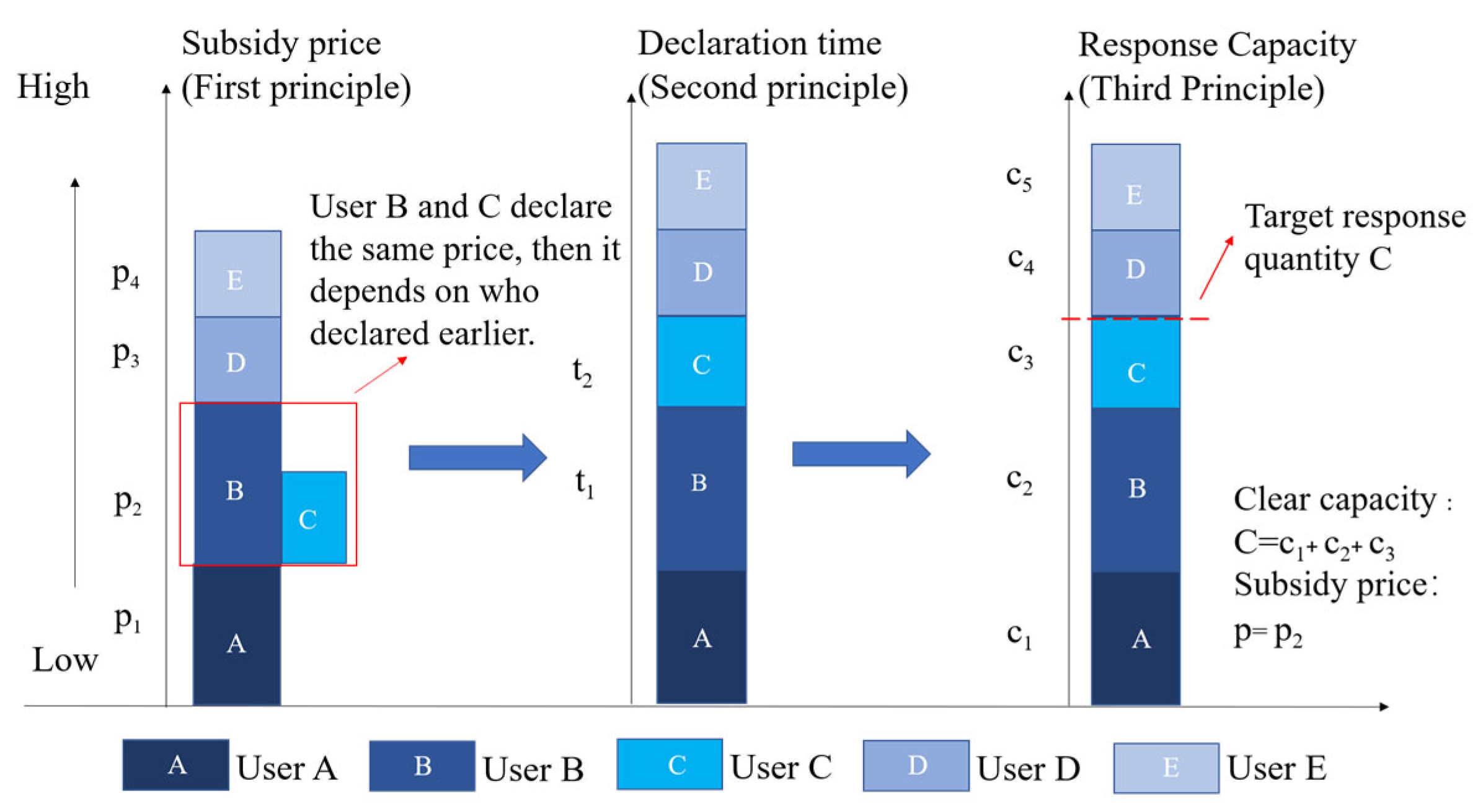
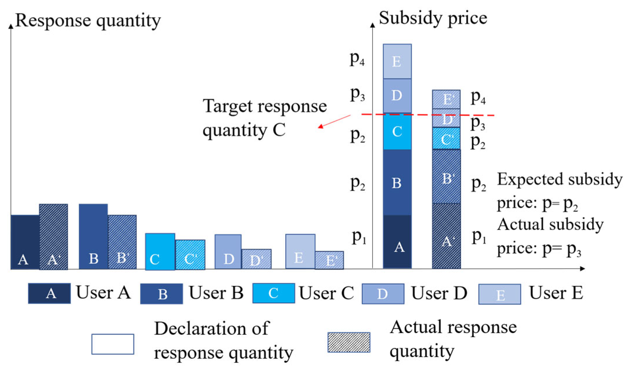
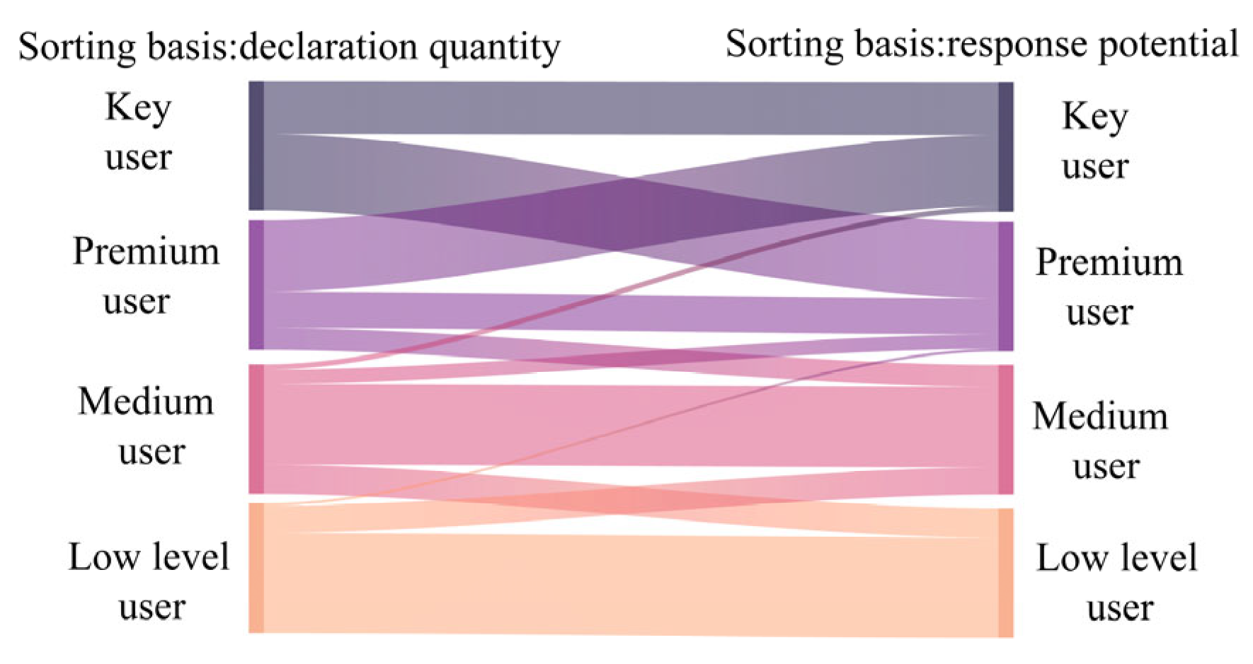
2.1. Analyzing the Process for Selecting Participating Users

This article describes the operational method of China’s DR using the DR document produced in Zhejiang Province, China, in May 2022 as an example [30]. Its specific operational structure is illustrated in Figure 1. After receiving the announcement, users and load aggregators declare their response quantity and ideal subsidy price. The power grid company determines the list of participating users and the subsidy price based on the principle of “Marginal Clearance”. According to data feedback, the effectiveness of China’s DR mechanism in actual operation is not rational [20].

Figure 2 depicts the “Marginal Clearance” rule. The declared users are sorted according to the rules of the declared price from low to high (First principle) and declared response quantity from high to low (Second principle). The declared response quantity of the top ranked users is included in the load resource pool until the cumulative response quantity reaches the target value. The declared price of the last successful bidding customer is the marginal clearing price. Because declared users are unable to precisely assess their response quantity throughout the response period, the principle of “Marginal Clearance” determines participating users based on their declared quantity, leading to a significant discrepancy between the target response quantity and the actual response quantity. Thus, studying how to make user declaration responses close to their actual response quantity and determine the list of participating users can help improve the existing DR mechanism.

2.2. Analysis of the Methodology for Determining Subsidy Price

The quantity of user response is affected by the subsidy price. Users’ desire to respond will be significantly impacted by the subsidy price if it is too low, and the power grid company will incur excessive response costs if the subsidy price is too high. The marginal price computed based on the “Marginal Clearance” principle cannot represent the expected price of users as the response quantity indicated by users cannot correctly reflect their actual response quantity, as is illustrated in Figure 3′s analysis. The subsidy price set by the power grid company is $p_2$, while the subsidy price based on the actual response quantity is $p_3$. The subsidy price $p_2$ determined by the power grid company is lower than the user’s ideal subsidy price $p_3$, which will make the user less willing to respond, resulting in the user’s actual response quantity being lower than the declared quantity.

In conclusion, there are certain issues with the current DR mechanism in determining the list of participating users and subsidy price. In terms of participating users, due to a lack of understanding of the user’s response potential, too many low-response potential users were invited, and the deviation between the response quantity declared by the user and the actual response quantity is significant, resulting in the inability of the power grid company to achieve its goals during DR and excessive redundancy in the number of participating users. In terms of subsidy price, the existing method for determining subsidy price cannot correctly reflect user’s ideal subsidy price, which weakens users’ willingness to participate in DR.

3. User DR Potential Prediction Model

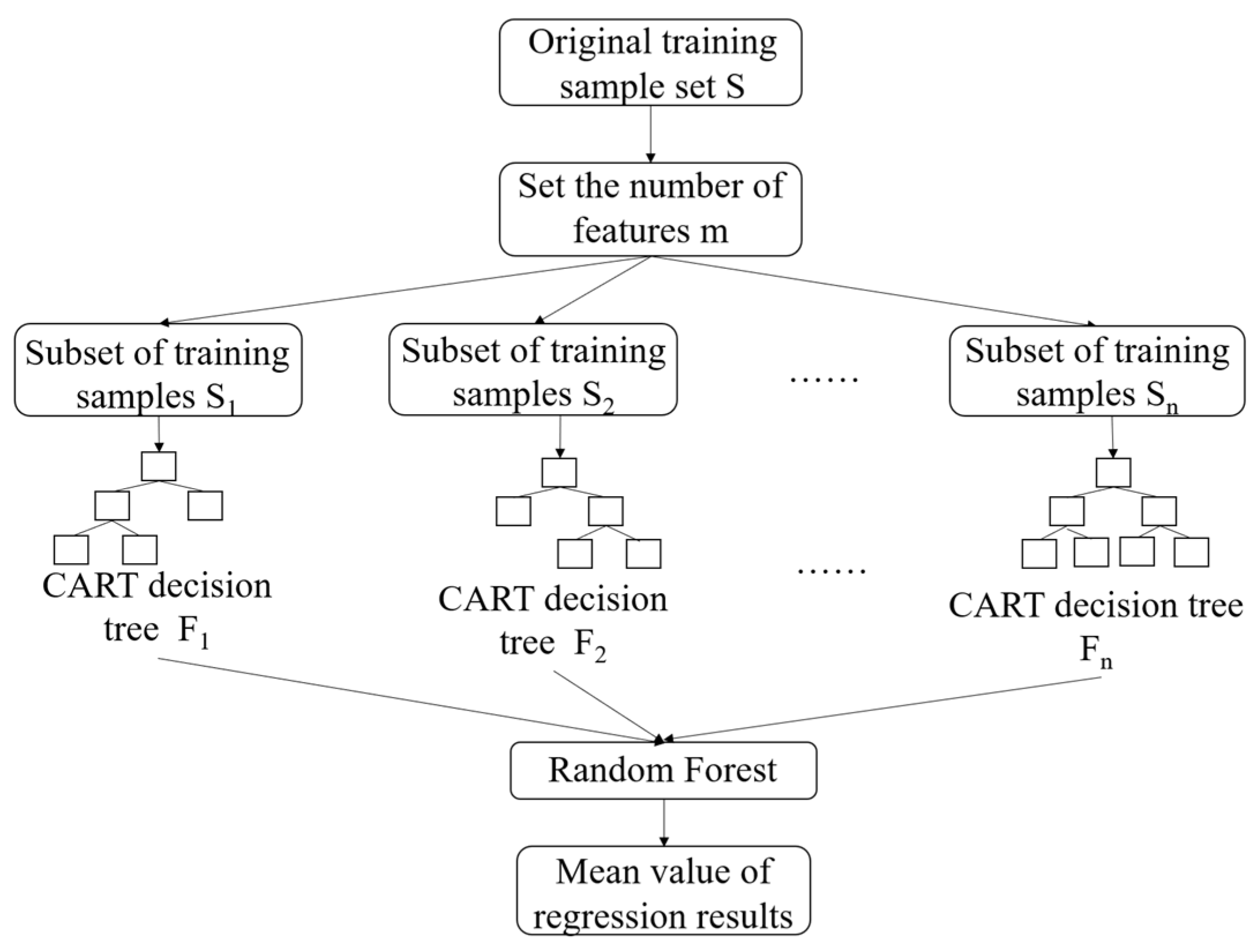
Integrated algorithms are made up of several algorithms that extract hidden information from enormous amounts of nonlinear and noisy data. The model developed using data-driven methods has good accuracy and a rapid computational speed [34]. The power grid company has a large amount of user electricity consumption behavior data. To identify user response potential, an integrated algorithm can be utilized to build a user response potential prediction model, and users can be ranked based on estimated response quantity.

3.1. RF Principle

Shi R. et al. [25] compared the accuracy of various machine learning methods in predicting user response quantity and found that the RF algorithm has the highest prediction accuracy due to its ability to reduce the risk of overfitting and fully consider the contribution of various feature variables. Therefore, this article uses the RF algorithm to construct a user response quantity prediction model.

For the original training sample set $S$ with the number of samples $N$ and the number of features $M$, the specific construction process of RF is shown in Figure 4, and the specific steps are as follows:

• Choose $m$ features at random from a pool of $M$ features; each sample’s feature dimension is $m$, where $m$ is less than $M$.
• Use the bootstrap method to perform repeated sampling on the training sample set $S$, generating $n$ training subsets $S_i$ ($i=1,2,\dots ,n$) of samples [35]. Out-of-bag (OOB) datasets are samples from the training sample set that do not appear in the subset being trained. OOB data make up roughly 36.8% of the training sample set [36].
• Create decision trees specifically for the training subset response quantities $S_i$ and obtain the RF model made up of $n$ decision trees.

The RF model developed in this paper consists of multiple categorical and regression trees (CARTs), where CART is a dichotomous recursive partitioning technique that splits the current sample set into two subsets at each node. For sample set $(x_i,y_i)$, the key to using CART for regression is to solve the following expression by identifying appropriate segmentation variables $m$ and segmentation sites $s$ to achieve the set threshold of the loss function:

$$\underset{m,s}{\min }[{\displaystyle \sum _{x_i\in D_l(m,s)}{(y_i-c_1)}^2+}{\displaystyle \sum _{x_i\in D_r(m,s)}{(y_i-c_2)}^2}]$$

(1)

where $D_l(m,s)$ and $D_r(m,s)$ denote the left and right subsets of the split; $c_1$ and $c_2$ are the average values of dataset $D_l(m,s)$ and $D_r(m,s)$, respectively.

The optimal decision tree can be generated by dividing the segmented subset according to Formula (1) until the set threshold is reached.

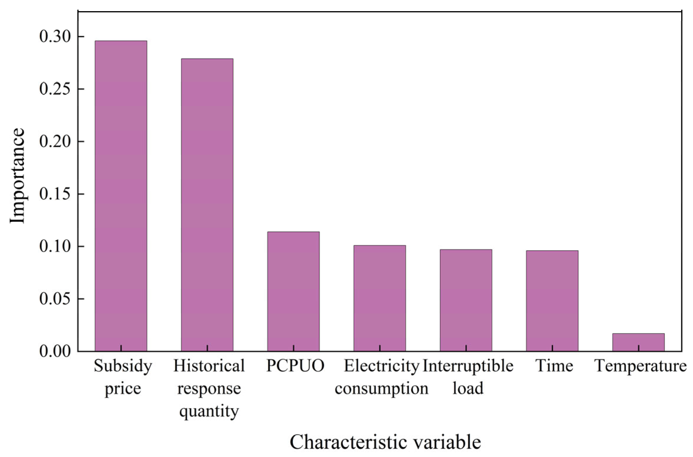
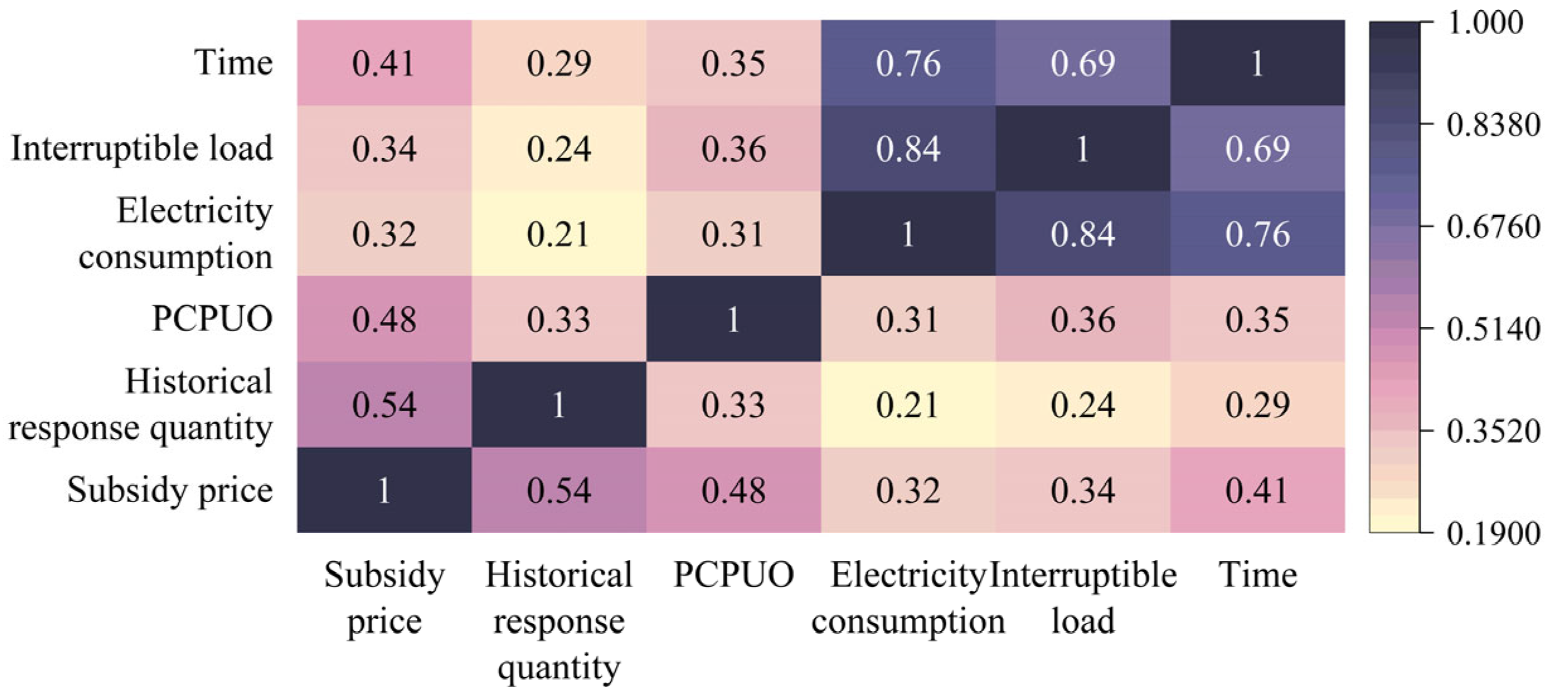
3.2. Feature Selection-Based Feature Variable Screening

Selecting accurate input feature variables is the primary condition for constructing a high-precision prediction model, so this paper adopts the RF feature selection algorithm to screen the key influencing factors.

The principle of determining the importance of feature variables in RF is to test the accuracy of the model using OOB data, then calculate the accuracy of the model after adding white noise to a certain feature variable and finally compare the accuracy before and after adding white noise. The feature variable is regarded as a crucial variable if the accuracy dramatically drops after adding white noise. If the accuracy fluctuates steadily after adding white noise, the feature variable is considered a non-critical variable. Below is an expression for the significance of the CV:

$$T_{m_i}=\frac{E_{oob}-E_{m_i}}{{\displaystyle \sum _{m_i\in M}{E}_{m_i}-E_{oob}}}$$

(2)

where $E_{oob}$ is the modeled original out-of-bag error; $E_{m_i}$ is the out-of-bag error after adding the noise value to the sample feature $m_i$.

Table 1. Summary of CV of related literatures.

Literature	CV	High Frequency CV
Shi R. et al. [25]	Electricity consumption PEC during response hours Interruptible load Subsidy price Range of fluctuations in electricity consumption	Subsidy price Historical response quantity Time Temperature Interruptible load Electricity consumption
Shirsat A. et al. [27]	Temperature Power usage Response time Temperature sensitivity
Kong X. et al. [26]	Response time Subsidy price Load baseline Actual load Temperature
Zhang Y. et al. [29]	Subsidy price Electricity consumption Historical response quantity Response time
Kong X. et al. [28]	Subsidy price Electricity consumption
Wohlfarth K. et al. [37]	Transferable load DR policies Subsidy price Customer willingness to respond Electricity load

lists the selected CVs from the literature for DR potential assessment. The variables used in each literature study are different, and a total of 13 different types of CVs appear in Table 1. If all 13 types of CVs are used as input variables, not only is it difficult to obtain data, but the model prediction accuracy is low. Therefore, in this paper, six CVs that appear more frequently in the existing literature are selected as candidate CVs, including subsidy price, time, temperature, interruptible load, electricity consumption, and historical response quantity. Most of the existing literature studies the CVs that affect the response quantity of residential users, but there are some differences in the response factors that affect industrial and residential users. Leinauer C. et al. [32] pointed out that power consumption per unit of output (PCPUO) and the benefits obtained from DR are the main factors affecting the response potential of industrial users. It is only when the proportion of electricity costs to total costs is large that users have a higher willingness to participate in DR. Therefore, this article takes the PCPUO into account based on six high-frequency CVs and ultimately selects seven CVs as candidate CVs. According to the DR implementation plan released by China and the related literature, the majority of the literature takes into account the subsidy price factor [28,29,31]. As a result, this article will prioritize the consideration of subsidy price, while other influencing factors will be determined through the RF feature selection algorithm.

3.3. An RF-Based Model for Evaluating User Response Potential

The steps for building a user response potential prediction model can be divided into the following steps:

• Select candidate input variables

This article summarizes the variables commonly used in the literature to predict user response quantity and selects variables with high frequency as candidate input variables, as shown in Table 1.

2.

Select important variables as input variables

RF has the function of evaluating the importance of each candidate input variable, and the principle of RF can be found in Section 3.1. This article uses the RF feature selection function to filter out the variables that have the greatest impact on user response potential, and the calculation expression is shown in Formula (2).

3.

Create an RF prediction model

This article uses the MATLAB machine learning toolbox (R2018b) to construct an RF prediction model. The RF algorithm analyzes the relationship between input variables and response quantity and constructs a user response potential prediction model. This article uses a tenfold cross-validation method to divide the dataset into a training set and testing set [38], with nine folds being used as the training set to train the model and the remaining one fold being used as the testing set to evaluate the accuracy of the model. The principle of the RF prediction model can be summarized as follows:

Given l samples in the test set, where $X_j(j=1,2,\dots l)$ is the jth input vector, the RF model’s $n$ decision trees forecast the DR of $X_j$, producing a set $L_j$ with $n$ predicted values. The expression is as follows:

$$L_j=\left\{F_1(X_j),F_2(X_j),\dots F_n(X_j)\right\}$$

(3)

The predicted value of the jth test set is the average of the predicted values of $n$ decision trees. The expression for the predicted value $f(\stackrel{\wedge }{X_j})$ is as follows:

$$f(\stackrel{\wedge }{X_j})=\frac{{\displaystyle \sum _{i=1}^n{F}_i(X_j)}}{n}$$

(4)

4.

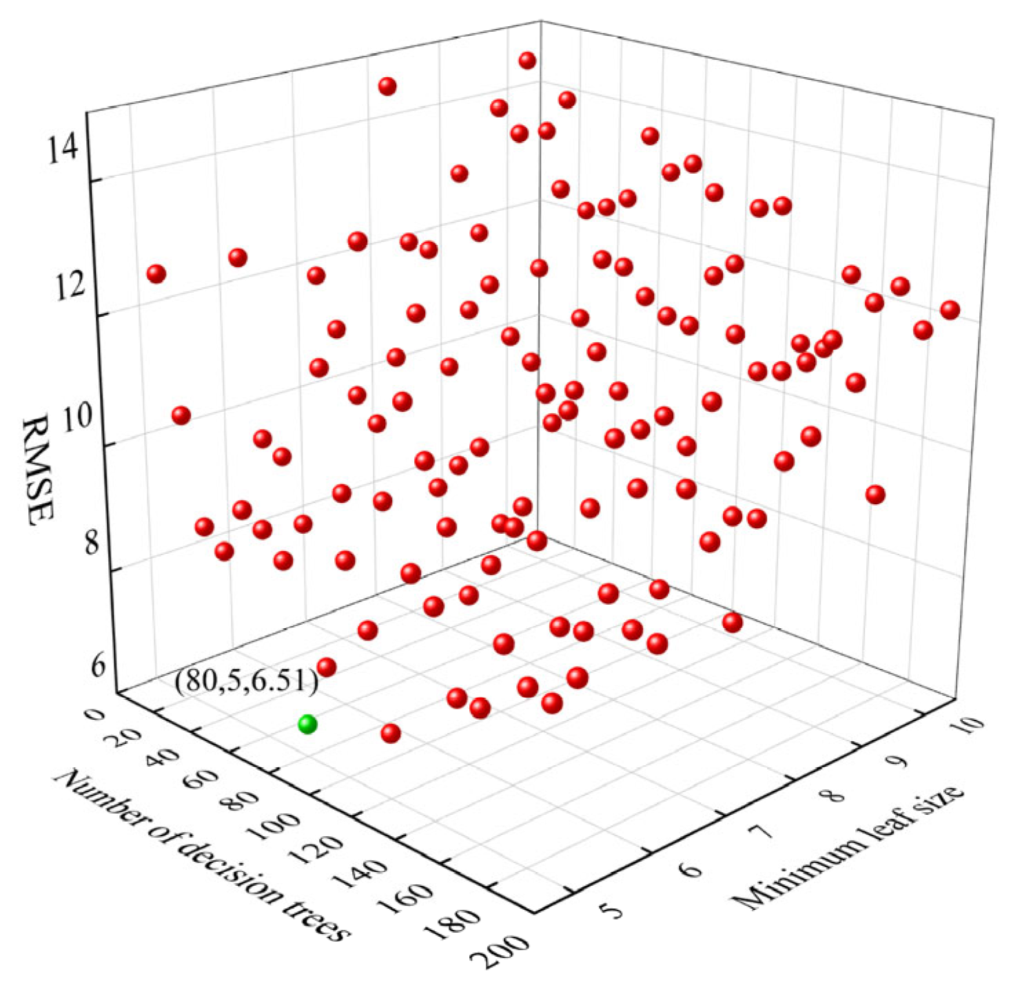
Search for the optimal parameter combination of the model

The RF prediction model constructed in this paper involves two parameters: the minimum leaf size (MLS) and the number of learning cycles (NLC). If the model parameters are not set appropriately, the model is prone to overfitting or underfitting. Therefore, it is necessary to determine the appropriate parameter combination to improve the accuracy of the model. The grid search searches for the best combination of parameters by traversing all possible combinations of given parameters in order to improve the accuracy of the model [39]. Therefore, this article uses the grid search method to adjust the model parameters. The root mean square error (RMSE) indicator can be selected as the evaluation criterion for the model’s predictive ability:

$$RMSE=\sqrt{\frac{{\displaystyle \sum _{j=1}^l(f(X_j)-\stackrel{\wedge }{f(X_j)}}{)}^2}{l}}$$

(5)

After the above four steps of operation, a high-prediction accuracy prediction model can be constructed. By inputting variable data such as subsidy price, it is feasible to predict the user’s response quantity in a certain period in the future.

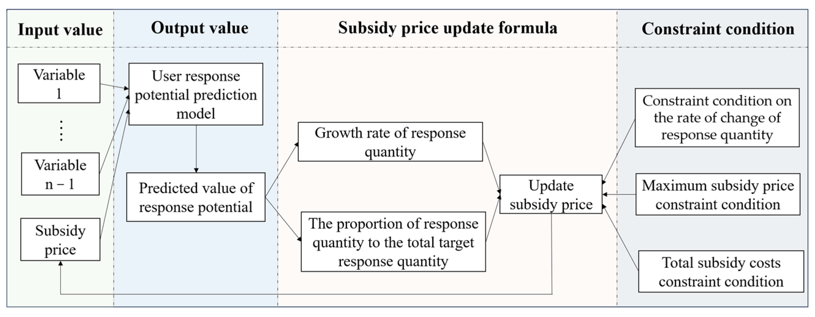
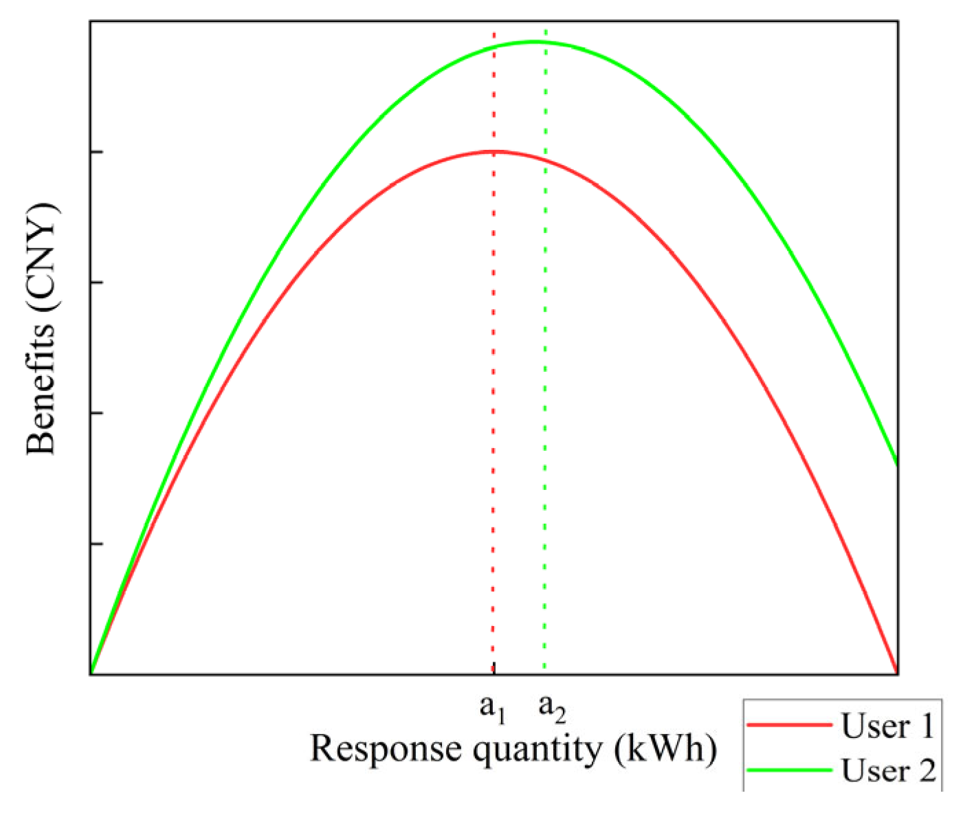
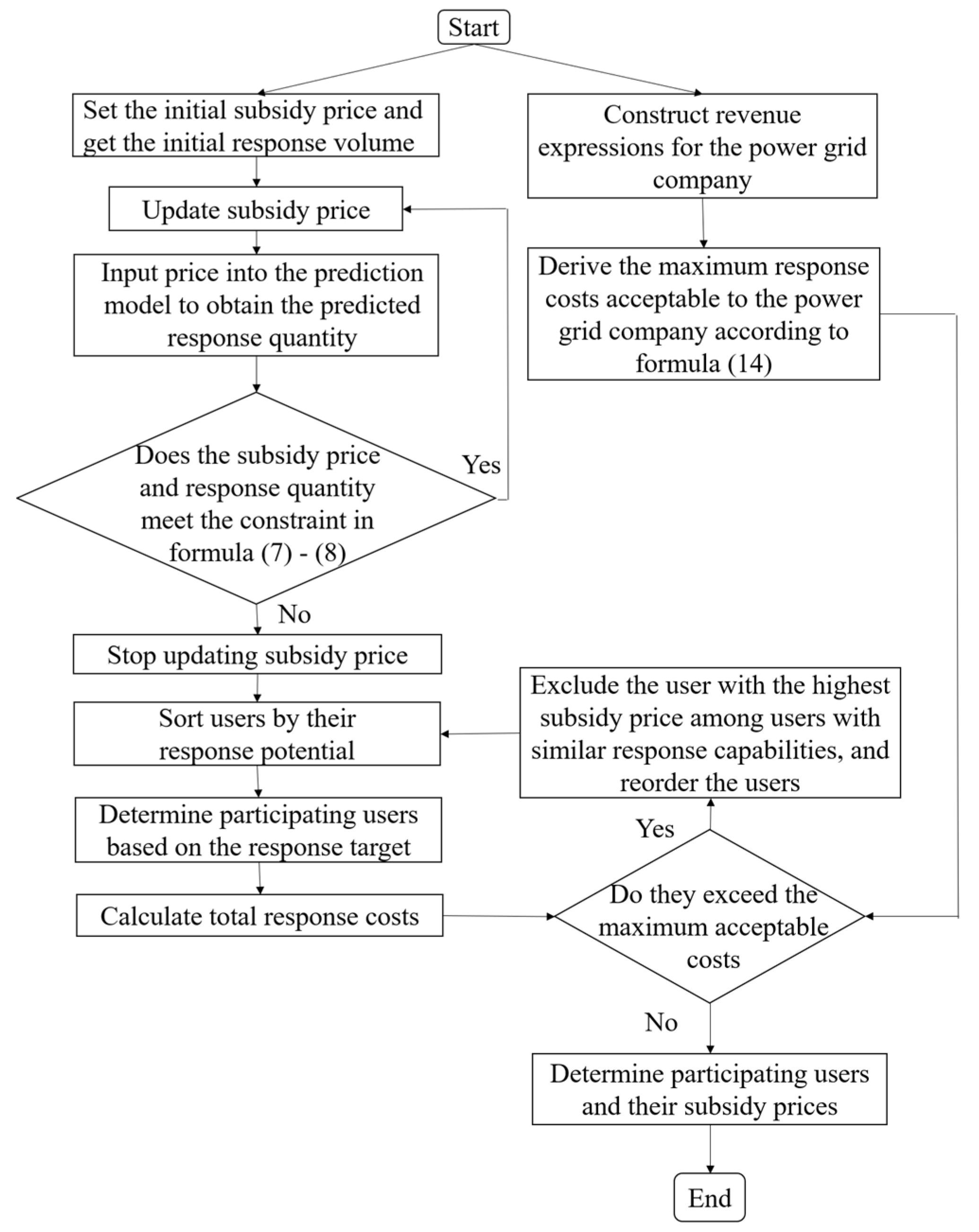
4. Differentiated Subsidy Price

Based on the response potential prediction model, this article formulates a differentiated subsidy price strategy, and the specific ideas for formulating a differentiated subsidy price strategy are shown in Figure 5. Figure 5 shows that after obtaining each user’s predicted response potential value, we utilize it to sequentially calculate the growth rate of user response quantity and the proportion of the user’s response quantity to target response quantity. These two parts are the main components of the differentiated subsidy price formula. In order to establish a reasonable subsidy price, this article sets a constraint condition on the rate of change of response quantity, maximum subsidy price constraint condition, and total subsidy costs constraint condition to dynamically adjust the subsidy price of each user.

4.1. Differentiated Subsidy Price Formula

The link between user benefits and response quantity can be represented by a quadratic function curve with a downward opening [40], as shown in Figure 6. When the response quantity is between $\left[0,a_1\right]$, the response willingness of the user is strong. When the response quantity exceeds $a_1$, the user’s lifestyle is disrupted, and the loss of comfort is greater than the response subsidy. Continuing to increase the subsidy price cannot significantly increase the user’s response quantity but instead increases the subsidy costs for the power grid company. Through the comparison in Figure 6, it is found that different users have different benefit functions, and their maximum response quantity varies. When users 1 and 2 reach their maximum response quantity, the subsidy price they receive should differ according to incentives and fairness theories. Therefore, it is necessary to develop a differentiated subsidy price strategy based on user’s response characteristics, further tapping into user response potential.

Initially, each user is assigned an equal subsidy price $p_{i,0}$, which is input into an RF prediction model to obtain the predicted response quantity $R_{i,0}$ of each user. The user subsidy price is then dynamically updated by accounting for the rate of user response quantity growth and the ratio of actual response quantity to target response quantity. The formula for differentiated subsidy price is as follows:

$$p_{i,t}=\left\{\begin{array}{l}{p}_{i,t-1}\times (1+\beta \times \frac{R_{i,t-1}}{R_{obj}}),t=1\hfill \\ p_{i,t-1}\times (1+\beta \times \frac{{R_{i,t-1}}^2}{R_{obj}\times R_{i,t-2}}),t>1\hfill \end{array}\right.$$

(6)

where $p_{i,t}$ represents the subsidy price received by user $i$ at the tth iteration; $R_{obj}$ represents the DR’s target response quantity; $R_{i,t}$ is the predicted response quantity of user $i$ at the tth iteration; and $\beta$ is the correction factor.

4.2. Constraint Conditions on the Subsidy Price Formula

4.2.1. Constraint Condition on the Rate of Change of Response Quantity

Each user’s response to changes in subsidy price varies. The user’s reaction is deemed to have reached its maximum potential value when the rate of change in response falls below a predetermined threshold. Continuing to raise the subsidy price will increase subsidy costs for the power grid company. Therefore, when the growth rate of user response quantity does not meet the constraint condition, we must stop updating the subsidy price for that user to avoid low-response potential users receiving excessive response subsidies. The expression for the constraint condition is as follows:

$$\frac{R_{i,t}-R_{i,t-1}}{R_{i,t-1}}\ge \gamma$$

(7)

where $\gamma$ is the growth rate threshold.

4.2.2. Maximum Subsidy Price Constraint Condition

When executing DR, the power grid company will determine the maximum subsidy price for users. Therefore, the subsidy price for users should be less than the maximum subsidy price, as expressed below:

$$p_i\le p_{\max }$$

(8)

where $p_{\max }$ is the maximum subsidy price set by the power grid company.

4.2.3. Total Subsidy Costs Constraint Condition

Before executing DR, it is necessary to estimate the maximum response costs that the power grid company can bear. This article deduces the maximum response costs by constructing profit formulas for the power grid company. The power grid company’s profit is primarily composed of three components during the DR implementation process: WPVP consumption revenue, thermal power unit ramp-up expenses, and DR subsidy costs.

• Benefits of WPVP consumption

Each province is required to meet the appropriate renewable energy consumption obligation weights and will be penalized if it does not, according to China’s Renewable Energy Power Consumption Guarantee Mechanism [41]. The benefits of increasing the consumption of WPVP through DR can be expressed as $C_{energy}$, where it is proportional to the increased WPVP consumption and the costs of WPVP abandonment [42].

$$C_{energy}={\displaystyle \sum _{t=1}^T(\mathsf{\Delta }{E}_t^{wind}+\mathsf{\Delta }{E}_t^{solar})\times c_p}$$

(9)

where $\mathsf{\Delta }{E}_t^{wind}$ and $\mathsf{\Delta }{E}_t^{solar}$ represent increased WPVP consumption; $c_p$ is the penalty costs coefficient for abandoned WPVP generation; and $T$ is the DR period.

2.

Climbing costs for thermal power units

Implementing DR can reduce the net load difference and climbing costs of thermal power units. This part of the costs is represented by $C_{climbing}$, which is directly proportional to the climbing costs coefficient of thermal power units and the change in net load curve power [42].

$$C_{climbing}={\displaystyle \sum _{t=1}^T{c}_q\times t\times \left|\mathsf{\Delta }{P}_{net,t}\right|}$$

(10)

$$P_{net,t}=P_{load,t}-P_{wind,t}-P_{solar,t}$$

(11)

where $P_{net,t}$ is the net load curve power at time $t$; $P_{load,t}$ denotes the load power at time $t$; $P_{wind,t}$ is the wind power generation power at time $t$; $P_{solar,t}$ is the PV power generation power at time $t$; and $c_q$ is the creeping costs factor for thermal power units.

3.

DR subsidy costs

In order to encourage users to change their electricity consumption behavior during the response period, the power grid company needs to be compensated for a certain portion of costs, denoted by $C_{dr}$, which is proportional to the subsidy price and amount of response power [42].

$$C_{dr}={\displaystyle \sum _{i=1}^N{\displaystyle \sum _{t=1}^T{R}_{i,t}}}\times p_i\times t$$

(12)

where $R_{i,t}$ is the response power of user $i$ at time $t$; $p_i$ is the subsidy price that user $i$ receives.

These three elements are added together to form the power grid company’s revenue.

$$P=C_{energy}+C_{climbing}-C_{dr}$$

(13)

This article assumes that users all aim to minimize electricity costs. In summer, the low electricity load period is generally from 11:30 to 14:30 and from 22:00 to 24:00. The electricity price during these two time periods is cheap, and users tend to transfer electricity to that period. Moreover, during these two time periods, there is remaining WPVP generation. Therefore, the increase in WPVP generation consumption is the amount of response load quantity. By making the profit formula of the power grid company bigger than zero, which is $P\ge 0$, the maximum acceptable response costs for the power grid company can be derived. The response costs constraint expression is as follows:

$$C_{dr}\le R_{obj}(c_p+2c_q)$$

(14)

where $R_{obj}$ represents the DR’s target response quantity.

The process of determining the users participating in DR and the differentiated subsidy price for each user are shown in Figure 7. Firstly, allocate initial subsidy price to each user and obtain the predicted initial response quantity for each user through the prediction model. Then, determine whether the output value meets the constraint conditions. Users who meet the constraint conditions continue to update their subsidy price. Otherwise, the subsidy price will be stopped from being updated. Next, after determining the subsidy price for each user, the final predicted response quantity for each user is obtained. Sort users based on the predicted response quantity and prioritize the participation of high-response potential users in DR. Finally, calculate the total response costs. If the total response costs exceed the expected value, the user with the highest subsidy price among users with similar response capabilities will be excluded and the users will be ranked again. When the total response costs are lower than the expected value, the subsidy price for the participating users and each user in this DR can be determined.

5. Model Effectiveness Evaluation Indicator System

The mismatch between the peak hours of WPVP generation and the peak hours of electricity demand has led to the waste of a large amount of WPVP to meet the power constraints of thermal power units. To address the previously mentioned problem, the research idea of this article is to use DR to maximize the overlap between the peak periods of WPVP generation and the peak periods of electricity load and reduce the peak–valley difference of electricity load in order to increase the consumption of WPVP. Therefore, this article designs the net load standard deviation (NLSD) index to reflect the overlap between the peak periods of WPVP generation and the peak periods of electricity demand. The peak–valley difference (PVD) index has been designed to reflect the peak–valley difference in electricity consumption. The goal of this article is to increase the consumption of WPVP, so the energy utilization rate (EUR) index has been designed to reflect the utilization rate of WPVP (see

Table 2. Physical meaning and direction of indicators.

Indicator	Physical Meaning	Direction
EUR	Reflecting the rate of WPVP consumption	Forward direction
NLSD	Reflect discrete trends in the net load curve	Negative direction
PVD	Reflect the range of net load curve spans	Negative direction

).

EUR: Ratio of WPVP consumption to total WPVP generation. The calculation formula is as follows [9]:

$$EUR=\frac{{\displaystyle \sum _{t=1}^T{E}_{t,usage}^{wind}}+{\displaystyle \sum _{t=1}^T{E}_{t,usage}^{solar}}}{{\displaystyle \sum _{t=1}^T{E}_t^{wind}}+{\displaystyle \sum _{t=1}^T{E}_t^{solar}}}\times 100\%$$

(15)

where ${\displaystyle \sum _{t=1}^T{E}_{t,usage}^{wind}}$ is the quantity of wind power consumed during the DR time period $T$; ${\displaystyle \sum _{t=1}^T{E}_{t,usage}^{solar}}$ is the quantity of PV power consumed during the DR time period $T$.

NLSD: The degree of deviation between the power of the net load curve and its mean. The calculation formula is as follows [9]:

$$NLSD=\sqrt{\frac{{\displaystyle \sum _{t=1}^T{(P_{net,t}-\overline{P_{net}})}^2}}{T}}$$

(16)

where $\overline{P_{net}}$ stands for the net load curve’s average power.

PVD: Net load curve peak-to-valley power difference. The calculation formula is as follows [9]:

$$PVD=P_{net,\max }-P_{net,\min }$$

(17)

where $P_{net,\max }$ denotes the maximum power value of the net load curve; $P_{net,\min }$ denotes the net load curve minimum power value.

6. Example Analysis

6.1. Data Sources

A total of 1893 industrial consumers in a city in East China were chosen as case study participants from the actual DR cases. The PCPUO refers to the U.S. report Oak Ridge National Lab [43]. The WPVP generation quantity was derived from the open-source dataset [44,45]. This study used the method proposed by Wang Y. et al. to obtain interruptible load [22], and the temperature was taken to be the average temperature of the response period on the response day. The user subsidy price, historical response quantity, electricity load, and declaration quantity were all derived from actual DR cases.

6.2. RF Modeling

In this study, we built an RF model using the MATLAB machine learning toolbox. The software defaults to setting the initial values of MLS and NLC to 8 and 30, respectively. The OOB data after adding white noise was fed into the model, and the results were normalized. Due to the randomness of white noise, in order to ensure the robustness of the results, it was repeated 30 times, and the average value was taken as the final result. The importance of each variable is shown in Figure 8. Figure 8 shows that subsidy price has the greatest impact on user response potential, which verifies the rationality of considering this factor in the current documents and literature. Temperature has a certain impact on response potential, but its importance is relatively low compared with other variables. From the perspective of data acquisition difficulty and model dimension, the temperature variable can be ignored.

The prediction model should be constructed to avoid the phenomenon of redundancy of feature information [37]. The Spearman correlation coefficient is a non-parametric statistical method that does not require any assumptions about the distribution of data [46]. Therefore, the Spearman correlation coefficient is used to calculate the correlation between feature variables and take the value in terms of absolute value. The results of the correlation between CVs are shown in Figure 9. It can be clearly seen from Figure 9 that electricity consumption, interruptible load, and time are highly correlated, so one variable can be used to replace the other two variables. Based on the difficulty of obtaining daily data, the power consumption is ultimately retained, while interruptible load and time are eliminated. In conclusion, this paper’s input variables include the subsidy price, historical response quantity, PCPUO, and power consumption.

This article uses the grid search method to obtain the ideal hyperparameter combination. When MLS and NLC are the default initial values of 8 and 30, respectively, the RMSE value of the model is 12.2. This article sets the value range of MLS to $\left[5,10\right]$ with a step size of 1 and the value range of NLC to $\left[10,200\right]$ with a step size of 10. The RMSE values of the model obtained by combining various parameter values are shown in Figure 10. From Figure 10, when MLS is set to 5 and NLC is set to 80, the RMSE value of the model is the smallest at 6.51, a decrease of 5.59 compared with the initial stage, effectively improving the prediction accuracy of the model. Due to the average response of the dataset in this article being 682 kWh, based on this value, the RMSE of the model is 6.51, indicating good predictive performance.

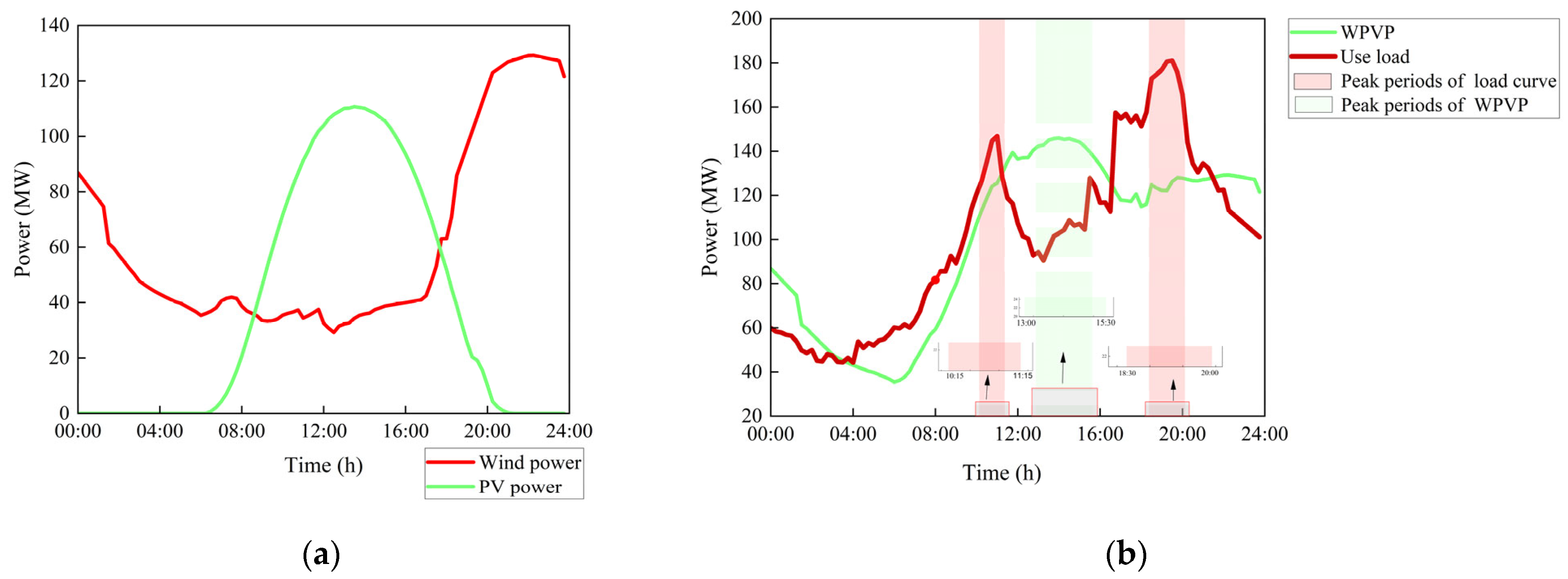
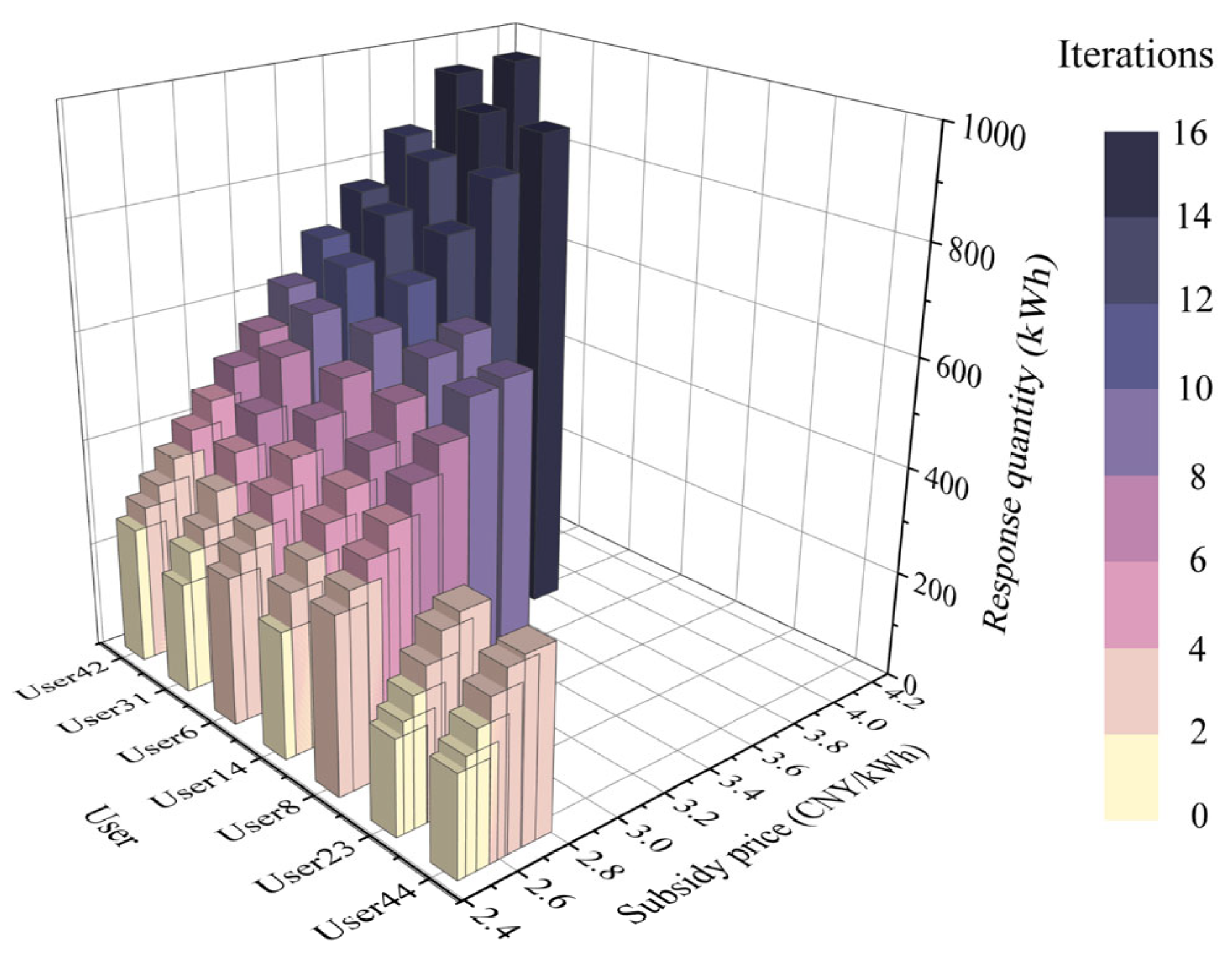
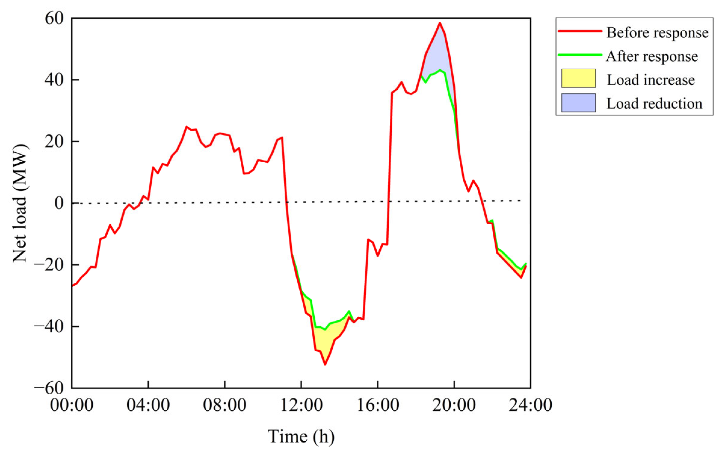
6.3. Analysis of WPVP Consumption

Compared with other seasons, the load curve in summer has the characteristics of short peak periods and large differences between peaks and valleys [47], resulting in low WPVP consumption in summer. As a result, the season of the example is set to summer to analyze the effect of this paper’s DR strategy on the consumption of WPVP. The WPVP curves are shown in Figure 11a, and the distribution of the WPVP curve and the user load curve with time is shown in Figure 11b. Figure 11b shows that the peak hours of electricity consumption are 10:15–11:15 and 18:30–20:00, while the peak hours for WPVP generation are 13:00–15:30, indicating a mismatch between the two peak times. To encourage the use of WPVP, this article implements a peak-shaving DR between 18:30 and 20:00, with an 80 MW load reduction target.

Referring to the DR implementation plans released by various provinces in China [30,31], we set the parameter values involved in the case as shown in

Table 3. Parameter symbols and values.

Parameter	Symbol	Numerical Value
Initial subsidy price	$p_0$	2.5 CNY/kWh
Maximum subsidy price	$p_{\max }$	4.5 CNY/kWh
Correction factor	$\beta$	2
Growth rate threshold	$\gamma$	0.1
Losses from WPVP penalty costs factor	$c_p$	1.75 CNY/kWh
Thermal power unit climbing costs coefficient	$c_q$	1.4 CNY/kWh

. The final subsidy price for each user can be determined through Formulas (6)–(8), and the response potential of each user can be determined by the user response potential prediction model. We sorted users based on their response potential, and the sorting results are shown in

Table 4. User sorting result.

Ranking	User	Response Quantity (MWh)	Accumulated Response Quantity (MWh)
1	User 42	0.955	0.955
2	User 31	0.914	1.869
3	User 6	0.905	2.774
4	User 282	0.891	3.665
……	……	……	……
141	User 221	0.296	79.226
142	User 352	0.292	79.518
143	User 367	0.288	79.806
144	User 210	0.284	80.090
145	User 320	0.282	80.372
146	User 224	0.281	80.653
……	……	……	……

. Table 4 shows that the cumulative response quantity of the top 144 users is 80.09 MWh, which meets the response target of 80 MWh. Therefore, the top 144 users will be prioritized for invitation to participate in DR. Equation (14) provides the maximum subsidy costs of the DR as CNY 364,000, and the power grid company pays a DR fee of CNY 247404, which is lower than the maximum subsidy fee and meets the constraint condition.

Due to the need for factories to develop precise production plans and execute DR at a certain period, some plans will be suspended. Therefore, they need to increase production efforts in the remaining time periods. To reflect the randomness of user load transfer, it is necessary to simulate the behavior of users transferring loads. The Monte Carlo method is a mathematical method based on probability theory and statistical theory that has been widely applied in simulating user electricity consumption behavior [48,49]. Therefore, this article uses Monte Carlo methods to simulate the behavior of users transferring response electricity to low electricity consumption periods. The Monte Carlo method will simulate user transfer behavior based on the response quantity of each user during the low periods of the total load curve. If the user’s electricity consumption at a certain moment during the low valley periods of the total load curve is higher than at other times during the low valley periods, the Monte Carlo method thinks with high probability that the user will transfer their electricity consumption to that period and uses this principle to simulate the user’s behavior of transferring electricity consumption. The change in net load curve before and after executing DR is shown in Figure 12, and the performance of DR in evaluation indicators is presented in

Table 5. Performance of DR in evaluation indicators.

Indicator	Before DR	After DR	Difference	Direction
EUR	81.17%	92.84%	11.67%	Forward direction
NLSD	27.01	24.32	−2.68	Negative direction
PVD	110.81	84.15	−26.66	Negative direction

.

Table 5 and Figure 12 show that after executing the DR, the net load curve becomes smoother, with the NLSD decreasing from 27.01 to 24.32, indicating that the supply–demand matching between the load curve and the WPVP generation curve has improved. By distributing part of the electricity consumption to low valley periods during peak load periods, the peak–valley gap narrows and the PVD drops from 110.81 to 84.15, further lessening the impact of the loss of WPVP brought on by climbing constraints for thermal power units. Based on the characteristics of WPVP generation, the low valley periods of electricity consumption overlap with the peak periods of WPVP generation. After implementing DR, the increase in electricity consumption during the low valley periods of electricity consumption promotes the consumption of remaining WPVP, resulting in an increase in the EUR index from 81.17% to 92.84%, an increase of nearly 12%.

6.4. An Analysis of the Effectiveness of DR Strategy

Sorting users according to the described response quantity is the basis of the “Marginal Clearance” principle. In order to demonstrate the effectiveness of the improvement strategy in this article, a comparative analysis will be conducted based on the results of sorting from different dimensions. Firstly, we sort the users by declaration quantity and response potential separately, with the upper, middle, and lower quantiles being nodes. Users are divided into “Key user”, “Premium user”, “Medium user”, and “Low level user”. The historical average of the user’s declaration quantity during the response periods is the declaration quantity utilized in this article. Some users whose declaration quantities are difficult to obtain are not included in this stage because of lacking data. The outcomes of the transformation of user labels are displayed in Figure 13. Figure 13 shows that when users are sorted by the dimension of “declared quantity”, certain users are ranked as “falsely high” or “falsely low”. Nearly 60% of users in the “Key user” tier are downgraded to “Premium user”, which indicates that these users overestimate their response potential and only judge response potential based on electricity consumption, resulting in an excessive declaration of response quantity. Nearly 50% of users in the “Premium user” tier have been upgraded to “Key users”, indicating that the majority of users have underestimated their response potential and received a corresponding reduction in response subsidies. After comparative analysis, it is found that the improvement strategy proposed in this article can reduce the gap between the target response quantity and the actual response quantity, helping users understand their response potential and the power grid company explore high-response potential users.

We further analyze the subsidy price received by each user and their response potential. Due to the large number of users, this article randomly selects a portion of users from various levels for display, as shown in Figure 14. It can be seen from Figure 14 that each user’s subsidy price is based on user’s response potential. After six iterations, user 44 was found to have earned the lowest subsidy price, 2.740 CNY/kWh, with a response potential of 334 kWh. User 42 received the highest subsidy price, 4.166 CNY/kWh, with a response potential of 955 kWh.

To clearly demonstrate the influence of differentiated subsidy price on user response potential, consumers are provided a uniform subsidy price of 3.5 CNY/kWh, which is compared with the approach of this study, and the results are shown in

Table 6. Comparison of the differentiated price and fixed price strategies.

	Differentiated Price Strategy			Fixed Price Strategy			Subsidy Costs Difference (CNY)
User	Response Quantity (kWh)	Subsidy Price (CNY/kWh)	Subsidy Costs (CNY)	Response Quantity (kWh)	Subsidy Price (CNY/kWh)	Subsidy Costs (CNY)
User 44	334	2.745	917	341	3.500	1194	−277
User 23	346	2.740	948	348	3.500	1218	−270
User 8	624	3.145	1962	629	3.500	2202	−240
User 14	648	3.219	2086	649	3.500	2271	−185
User 6	905	3.799	3438	824	3.500	2884	554
User 31	914	3.760	3436	831	3.500	2909	527
User 42	955	4.166	3978	784	3.500	2744	1234

. Table 6 demonstrates that while all users receive the same subsidy price under fixed price incentives, there is a significant variation in response quantity, with a maximum value of 784 kWh and a minimum value of 341 kWh, resulting in a difference of 443 kWh. Excessive ineffective response costs are spent on low potential users. According to the differentiated subsidy pricing strategy, due to the lower response potential of users 44, 23, 8, and 14 compared with other users, their subsidy price has decreased and the cumulative response subsidy has decreased by CNY 972. Users 6, 31, and 42 have higher response potential and, therefore, they receive higher subsidy prices, increasing their willingness to respond. Compared with the fixed subsidy price, their response quantity has increased by 335 kWh. Through comparative analysis, it can be concluded that the differentiation strategy can effectively reduce the costs of ineffective subsidy compared with fixed strategy and allocate more response subsidy to high-response potential users, further tapping into their response potential.

7. Conclusions

In order to improve the consumption of WPVP in the new power system, this article improves the existing DR strategy from two dimensions: the list of participating users and the subsidy price. This article constructs a user DR potential ranking model and formulates the differentiated subsidy price strategy based on user response characteristics. The case analysis shows that in terms of participating users, existing DR policies that rank users based on declaration quantity will result in some users ranking “falsely high” or “falsely low”. Among them, nearly 60% of users in the “Key user” level will be downgraded to “Premium user” level, and nearly 50% of users in the “Premium user” level will be upgraded to “Key user” level, indicating that users cannot accurately estimate their own response potential. In order to reduce the discrepancy between declared and real response quantity, this article suggests a user response potential sorting queue based on the prediction model. This allows users to declare response quantity more fairly when engaging in DR and prioritize inviting high-response potential users to participate in DR. In terms of subsidy price, this article suggests constraint conditions and a subsidy price update formula that take user response characteristics into account. Compared with the fixed price strategy, differentiated subsidy price is determined by the response potential of users. Due to significant differences in users’ response potential, the maximum subsidy price difference between users can reach 1.467 CNY/kWh. The subsidy costs for low-response potential users have cumulatively decreased by CNY 971. High potential users have received more subsidies, which has prompted them to increase their response quantity, resulting in a cumulative increase of 335 kWh in response quantity. Therefore, differentiated subsidy prices can be used to further tap into the response potential of users and maintain the principle of fairness.

By improving both the list of participating users and the subsidy price, the net load curve is smoother compared with the original DR strategy. The electricity consumption during peak hours has been distributed to low periods, narrowing the gap between the electricity consumption during peak periods and low periods, and the NLSD has dropped from 27.01 to 24.32. The load curve and WPVP power generation curve now match better in terms of supply and demand, resulting in a nearly 12% increase in the consumption rate of WPVP. Overreliance on coal for power generation poses great harm to the global environment, and vigorously developing renewable energy generation has become a consensus and action for countries around the world to promote sustainable development. In order to promote the process of sustainable development, this article studied how to further improve the utilization rate of renewable energy generation such as wind power and PV power and contribute to the early realization of sustainable development goals in the world.

This article uses DR to transfer the load from peak periods to low periods in order to improve the overlap between peak electricity load periods and peak WPVP generation periods. However, if many users transfer their electricity load to the same period, it is easy to generate new peak load periods, which will have a huge impact on the safety and electricity costs of the power grid system. In the future, based on the research in this article, we will consider introducing a third-party entity—load aggregator—and constructing a more corresponding model to address this issue. Our objective is to ensure the stability of the power system while advancing the utilization rate of renewable energy sources.

References

1. National Energy Administration. Presentation of Renewable Energy Grid Connected Operations in 2018. Available online: http://www.nea.gov.cn/2019-01/28/c_137780519.htm (accessed on 14 July 2023).
2. National Energy Administration. National Energy Administration Releases National Electric Power Industry Statistics for January-September. Available online: http://www.nea.gov.cn/202210/24/c_1310670890.htm (accessed on 14 July 2023).
3. Wang, Q.; Chang, P.; Bai, R.; Liu, W.; Dai, J.; Tang, Y. Mitigation Strategy for Duck Curve in High Photovoltaic Penetration Power System Using Concentrating Solar Power Station. Energies 2019, 12, 3521. [Google Scholar] [CrossRef]
4. Li, W.; Dong, F.; Ji, Z.; Ji, L. Evaluation of Provincial Power Supply Reliability with High Penetration of Renewable Energy Based on Combination Weighting of Game Theory-TOPSIS Method. Sustain. Energy Grids Netw. 2023, 35, 101092. [Google Scholar] [CrossRef]
5. Zhang, G.; Niu, Y.; Xie, T.; Zhang, K. Multi-Level Distributed Demand Response Study for a Multi-Park Integrated Energy System. Energy Rep. 2023, 9, 2676–2689. [Google Scholar] [CrossRef]
6. Leherbauer, D.; Hehenberger, P. Physics-Based Modeling and Parameter Tracing for Industrial Demand-Side Management Applications: A Novel Approach. Sustainability 2024, 16, 1995. [Google Scholar] [CrossRef]
7. Yan, Q.; Lin, H.; Zhang, M.; Ai, X.; Gejirifu, D.; Li, J. Two-Stage Flexible Power Sales Optimization for Electricity Retailers Considering Demand Response Strategies of Multi-Type Users. Int. J. Electr. Power Energy Syst. 2022, 137, 107031. [Google Scholar] [CrossRef]
8. Jiangsu Provincial Development and Reform Commission. Regarding the public solicitation of the Implementation Rules for Jiangsu Province’s Electricity Demand Response. Available online: https://fzggw.jiangsu.gov.cn/art/2022/10/24/art_284_10637935.html (accessed on 14 July 2023).
9. Cai, Q.; Xu, Q.; Qing, J.; Shi, G.; Liang, Q.-M. Promoting Wind and Photovoltaics Renewable Energy Integration through Demand Response: Dynamic Pricing Mechanism Design and Economic Analysis for Smart Residential Communities. Energy 2022, 261, 125293. [Google Scholar] [CrossRef]
10. Fan, S.; Li, Z.; Yang, L.; He, G. Customer Directrix Load-Based Large-Scale Demand Response for Integrating Renewable Energy Sources. Electr. Power Syst. Res. 2020, 181, 106175. [Google Scholar] [CrossRef]
11. Xu, H.; Chang, Y.; Zhao, Y.; Wang, F. A New Multi-Timescale Optimal Scheduling Model Considering Wind Power Uncertainty and Demand Response. Int. J. Electr. Power Energy Syst. 2023, 147, 108832. [Google Scholar] [CrossRef]
12. Zhao, X.; Bai, Z.; Xue, W.; Xu, N.; Li, C.; Zhao, H. Research on Bi-Level Cooperative Robust Planning of Distributed Renewable Energy in Distribution Networks Considering Demand Response and Uncertainty. Energy Rep. 2021, 7, 1025–1037. [Google Scholar] [CrossRef]
13. Cai, T.; Dong, M.; Liu, H.; Nojavan, S. Integration of Hydrogen Storage System and Wind Generation in Power Systems under Demand Response Program: A Novel p-Robust Stochastic Programming. Int. J. Hydrogen Energy 2022, 47, 443–458. [Google Scholar] [CrossRef]
14. Dai, X.; Li, Y.; Zhang, K.; Feng, W. A Robust Offering Strategy for Wind Producers Considering Uncertainties of Demand Response and Wind Power. Appl. Energy 2020, 279, 115742. [Google Scholar] [CrossRef]
15. Lu, X.; Ge, X.; Li, K.; Wang, F.; Shen, H.; Tao, P.; Hu, J.; Lai, J.; Zhen, Z.; Shafie-khah, M.; et al. Optimal Bidding Strategy of Demand Response Aggregator Based On Customers’ Responsiveness Behaviors Modeling Under Different Incentives. IEEE Trans. Ind. Appl. 2021, 57, 3329–3340. [Google Scholar] [CrossRef]
16. Baharlouei, Z.; Hashemi, M.; Narimani, H.; Mohsenian-Rad, H. Achieving Optimality and Fairness in Autonomous Demand Response: Benchmarks and Billing Mechanisms. IEEE Trans. Smart Grid 2013, 4, 968–975. [Google Scholar] [CrossRef]
17. Baharlouei, Z.; Hashemi, M. Efficiency-Fairness Trade-off in Privacy-Preserving Autonomous Demand Side Management. IEEE Trans. Smart Grid 2014, 5, 799–808. [Google Scholar] [CrossRef]
18. Liu, D.; Qin, Z.; Hua, H.; Ding, Y.; Cao, J. Incremental Incentive Mechanism Design for Diversified Consumers in Demand Response. Appl. Energy 2023, 329, 120240. [Google Scholar] [CrossRef]
19. Hamidpour, H.; Aghaei, J.; Dehghan, S.; Pirouzi, S.; Niknam, T. Integrated Resource Expansion Planning of Wind Integrated Power Systems Considering Demand Response Programmes. IET Renew. Power Gener. 2019, 13, 519–529. [Google Scholar] [CrossRef]
20. Lishui Development and Reform Commission. Announcement on Special Market Trial Operation Response Subsidies for Power Load Response. Available online: http://fgw.lishui.gov.cn/art/2021/10/9/art_1229228449_4749295.html (accessed on 1 April 2024).
21. Pang, Y.; He, Y.; Jiao, J.; Cai, H. Power Load Demand Response Potential of Secondary Sectors in China: The Case of Western Inner Mongolia. Energy 2020, 192, 116669. [Google Scholar] [CrossRef]
22. Wang, Y.; Li, F.; Yang, J.; Zhou, M.; Song, F.; Zhang, D.; Xue, L.; Zhu, J. Demand Response Evaluation of RIES Based on Improved Matter-Element Extension Model. Energy 2020, 212, 118121. [Google Scholar] [CrossRef]
23. Wang, T.; Wang, J.; Zhao, Y.; Shu, J.; Chen, J. Multi-Objective Residential Load Dispatch Based on Comprehensive Demand Response Potential and Multi-Dimensional User Comfort. Electr. Power Syst. Res. 2023, 220, 109331. [Google Scholar] [CrossRef]
24. Giannelos, S.; Konstantelos, I.; Strbac, G. Option Value of Demand-Side Response Schemes Under Decision-Dependent Uncertainty. IEEE Trans. Power Syst. 2018, 33, 5103–5113. [Google Scholar] [CrossRef]
25. Shi, R.; Jiao, Z. Individual Household Demand Response Potential Evaluation and Identification Based on Machine Learning Algorithms. Energy 2023, 266, 126505. [Google Scholar] [CrossRef]
26. Kong, X.; Wang, Z.; Liu, C.; Zhang, D.; Gao, H. Refined Peak Shaving Potential Assessment and Differentiated Decision-Making Method for User Load in Virtual Power Plants. Appl. Energy 2023, 334, 120609. [Google Scholar] [CrossRef]
27. Shirsat, A.; Tang, W. Quantifying Residential Demand Response Potential Using a Mixture Density Recurrent N-eural Network. Int. J. Electr. Power Energy Syst. 2021, 130, 106853. [Google Scholar] [CrossRef]
28. Kong, X.; Kong, D.; Yao, J.; Bai, L.; Xiao, J. Online Pricing of Demand Response Based on Long Short-Term Memory and Reinforcement Learning. Appl. Energy 2020, 271, 114945. [Google Scholar] [CrossRef]
29. Zhang, Y.; Ai, Q.; Li, Z. ADMM-based Distributed Response Quantity Estimation: A Probabilistic Perspective. IET Gener. Transm. Distrib. 2020, 14, 6594–6602. [Google Scholar] [CrossRef]
30. Zhejiang Provincial Development And Reform Commission. Notice of Electricity Demand Response for 2021. Available online: https://fzggw.zj.gov.cn/art/2021/6/8/art_1229629046_4906648.html (accessed on 14 July 2023).
31. North Star Power Grid. Chongqing Grid Demand Response Implementation Program in 2022 (Trial). Available online: https://news.bjx.com.cn/html/20220518/1225886.shtml (accessed on 14 July 2023).
32. Leinauer, C.; Schott, P.; Fridgen, G.; Keller, R.; Ollig, P.; Weibelzahl, M. Obstacles to Demand Response: Why Industrial Companies Do Not Adapt Their Power Consumption to Volatile Power Generation. Energy Policy 2022, 165, 112876. [Google Scholar] [CrossRef]
33. Monfared, H.J.; Ghasemi, A.; Loni, A.; Marzband, M. A Hybrid Price-Based Demand Response Program for the Residential Micro-Grid. Energy 2019, 185, 274–285. [Google Scholar] [CrossRef]
34. Shi, W.; Ma, X.; Min, Y.; Yang, H. Feasibility Analysis of Indirect Evaporative Cooling System Assisted by Liquid Desiccant for Data Centers in Hot-Humid Regions. Sustainability 2024, 16, 2011. [Google Scholar] [CrossRef]
35. Karabadji, N.E.I.; Amara Korba, A.; Assi, A.; Seridi, H.; Aridhi, S.; Dhifli, W. Accuracy and Diversity-Aware Multi-Objective Approach for Random Forest Construction. Expert Syst. Appl. 2023, 225, 120138. [Google Scholar] [CrossRef]
36. Zhou, Z. Machine Learning; Tsinghua University Press: Beijing, China, 2016; pp. 171–180. [Google Scholar]
37. Wohlfarth, K.; Klobasa, M.; Gutknecht, R. Demand Response in the Service Sector—Theoretical, Technical and Practical Potentials. Appl. Energy 2020, 258, 114089. [Google Scholar] [CrossRef]
38. Inan, O. A Method of Classification Performance Improvement Via a Strategy of Clustering-Based Data Elimination Integrated with k-Fold Cross-Validation. Arab. J. Sci. Eng. 2021, 46, 1199–1212. [Google Scholar] [CrossRef]
39. Sun, Y.; Ding, S.; Zhang, Z.; Jia, W. An Improved Grid Search Algorithm to Optimize SVR for Prediction. Soft Comput. 2021, 25, 5633–5644. [Google Scholar] [CrossRef]
40. Pradhan, V.; Murthy Balijepalli, V.S.K.; Khaparde, S.A. An Effective Model for Demand Response Management Systems of Residential Electricity Consumers. IEEE Syst. J. 2016, 10, 434–445. [Google Scholar] [CrossRef]
41. National Energy Administration. Notice on Establishing and Improving the Renewable Energy Electricity Consumption Guarantee Mechanism. Available online: https://www.gov.cn/zhengce/zhengceku/2019-09/25/content_5432993.htm (accessed on 14 July 2023).
42. Tan, Z.; Ju, L.; Reed, B.; Rao, R.; Peng, D.; Li, H.; Pan, G. The Optimization Model for Multi-Type Customers Assisting Wind Power Consumptive Considering Uncertainty and Demand Response Based on Robust Stochastic Theory. Energy Convers. Manag. 2015, 105, 1070–1081. [Google Scholar] [CrossRef]
43. Oak Ridge National Lab. 2013; Assessment of Industrial Load for Demand Response across U.S. Regions of the Western Interconnect. Available online: https://info.ornl.gov/sites/publications/files/Pub45942.pdf (accessed on 14 July 2023).
44. Elia Transmission Belgium SA. Solar Power Generation. Elia. Available online: https://www.elia.be/en/grid-data/power-generation/solar-pv-power-generation-data (accessed on 14 July 2023).
45. Elia Transmission Belgium SA. Wind Power Generation. Elia. Available online: https://www.elia.be/en/grid-data/power-generation/wind-power-generation?csrt=9625836695571506098 (accessed on 14 July 2023).
46. Omar, N.; Aly, H.; Little, T. Optimized Feature Selection Based on a Least-Redundant and Highest-Relevant Framework for a Solar Irradiance Forecasting Model. IEEE Access 2022, 10, 48643–48659. [Google Scholar] [CrossRef]
47. Wang, Y.; Rui, L.; Ma, J.; Jin, Q. A Short-Term Residential Load Forecasting Scheme Based on the Multiple Correlation-Temporal Graph Neural Networks. Appl. Soft Comput. 2023, 146, 110629. [Google Scholar] [CrossRef]
48. Iwafune, Y.; Ogimoto, K.; Kobayashi, Y.; Murai, K. Driving Simulator for Electric Vehicles Using the Markov Chain Monte Carlo Method and Evaluation of the Demand Response Effect in Residential Houses. IEEE Access 2020, 8, 47654–47663. [Google Scholar] [CrossRef]
49. Bottaccioli, L.; Di Cataldo, S.; Acquaviva, A.; Patti, E. Realistic Multi-Scale Modeling of Household Electricity Behaviors. IEEE Access 2019, 7, 2467–2489. [Google Scholar] [CrossRef]
Figure 1. DR framework diagram.
Sustainability 16 03248 g001
Figure 2. “Marginal Clearance” rule.
Sustainability 16 03248 g002
Figure 3. Analysis of the “Marginal Clearance” rule.
Sustainability 16 03248 g003
Figure 4. RF construction process.
Sustainability 16 03248 g004
Figure 5. Methodology for setting the subsidy price strategy.
Sustainability 16 03248 g005
Figure 6. Relationship between user revenue and response quantity.
Sustainability 16 03248 g006
Figure 7. The process of determining participating users and subsidy price.
Sustainability 16 03248 g007
Figure 8. Importance ranking of feature variables.
Sustainability 16 03248 g008
Figure 9. Correlation coefficient between CVs.
Sustainability 16 03248 g009
Figure 10. Comparison of the RMSE for each parameter combination.
Sustainability 16 03248 g010
Figure 11. WPVP curve and user load curve.
Sustainability 16 03248 g011
Figure 12. Changes in net load curve before and after DR.
Sustainability 16 03248 g012
Figure 13. The results of user labeling conversion.
Sustainability 16 03248 g013
Figure 14. The subsidy price and response potential of users.
Sustainability 16 03248 g014