
Spatio-Temporal Variation in Landforms and Surface Urban Heat Island in Riverine Megacity

 ,
,  , and
, and
Abstract
:1. Introduction
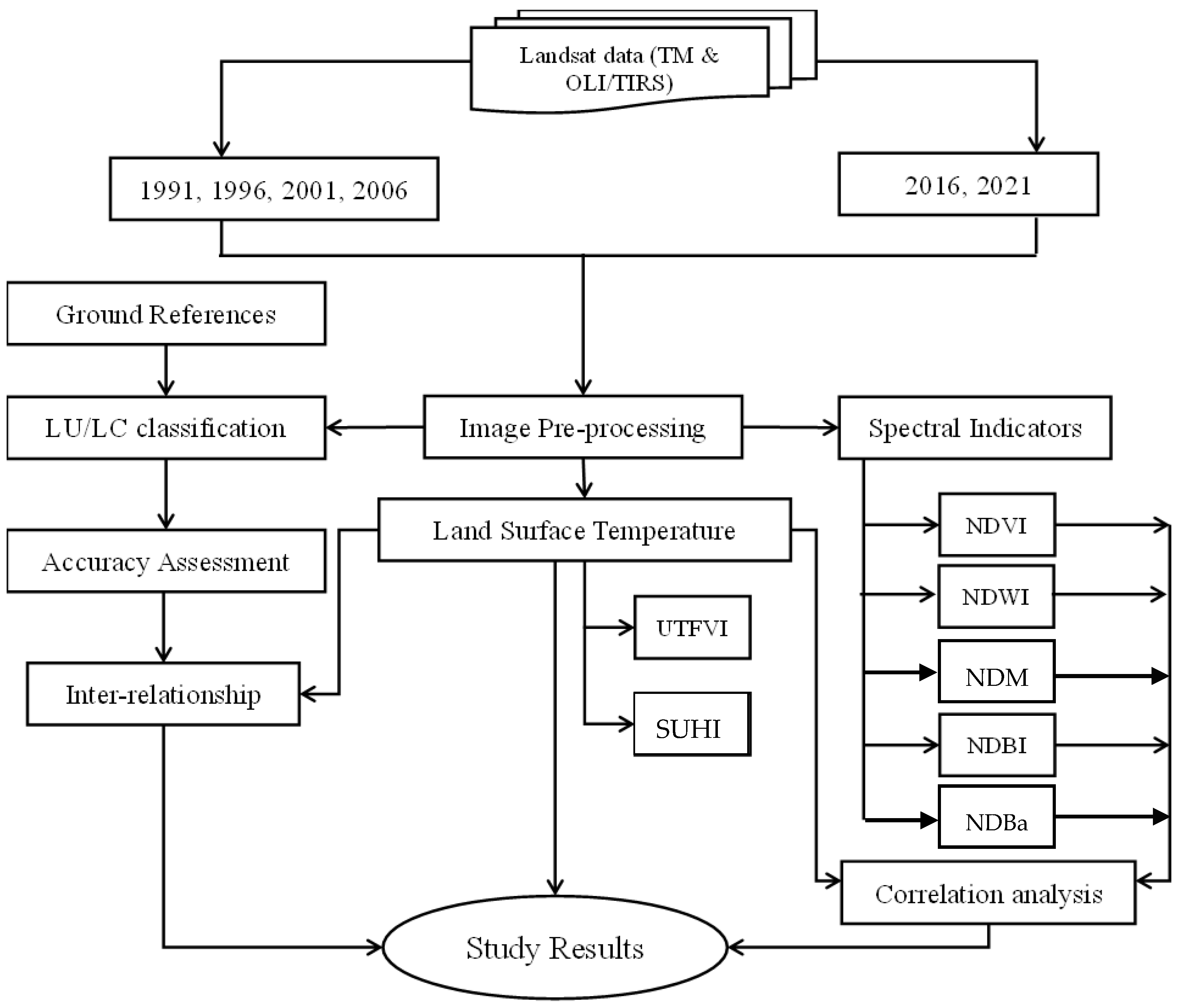
2. Materials and Methods
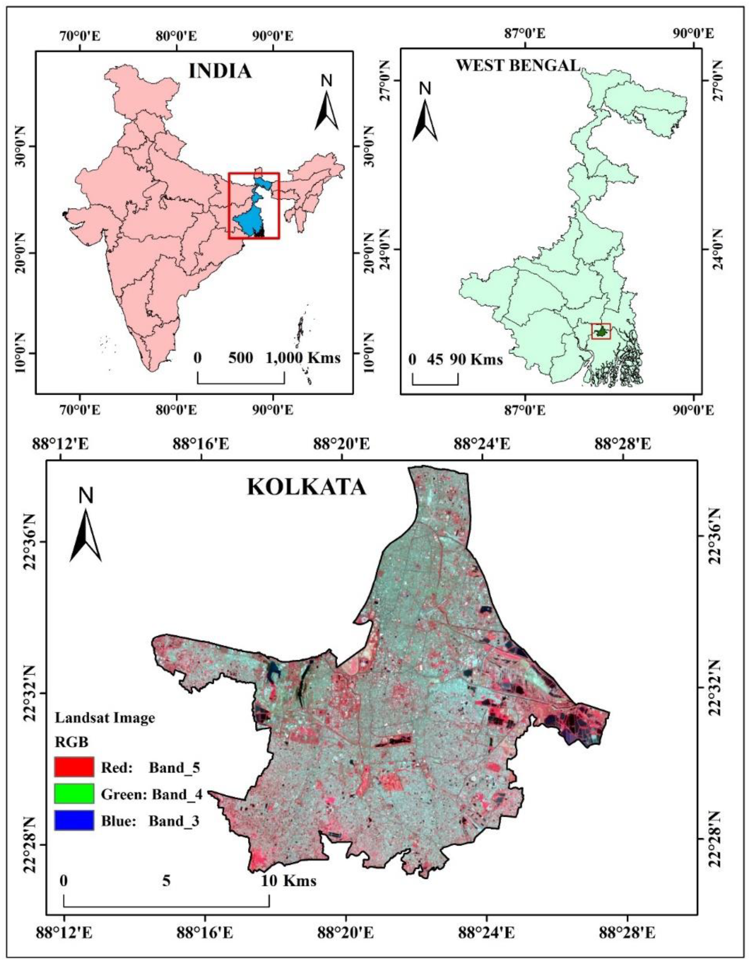
2.1. Study Area
2.2. Applied Datasets
2.3. Image Pre-Processing and Classification
2.4. Accuracy Assessment and Kappa Statistic
2.5. Geo-Spatial Indices
2.5.1. NDVI
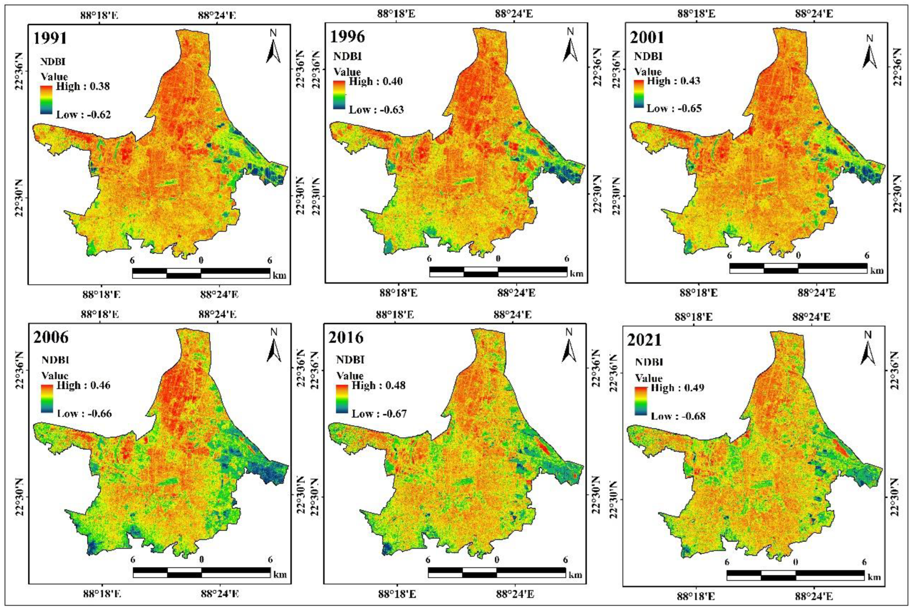
2.5.2. NDBI
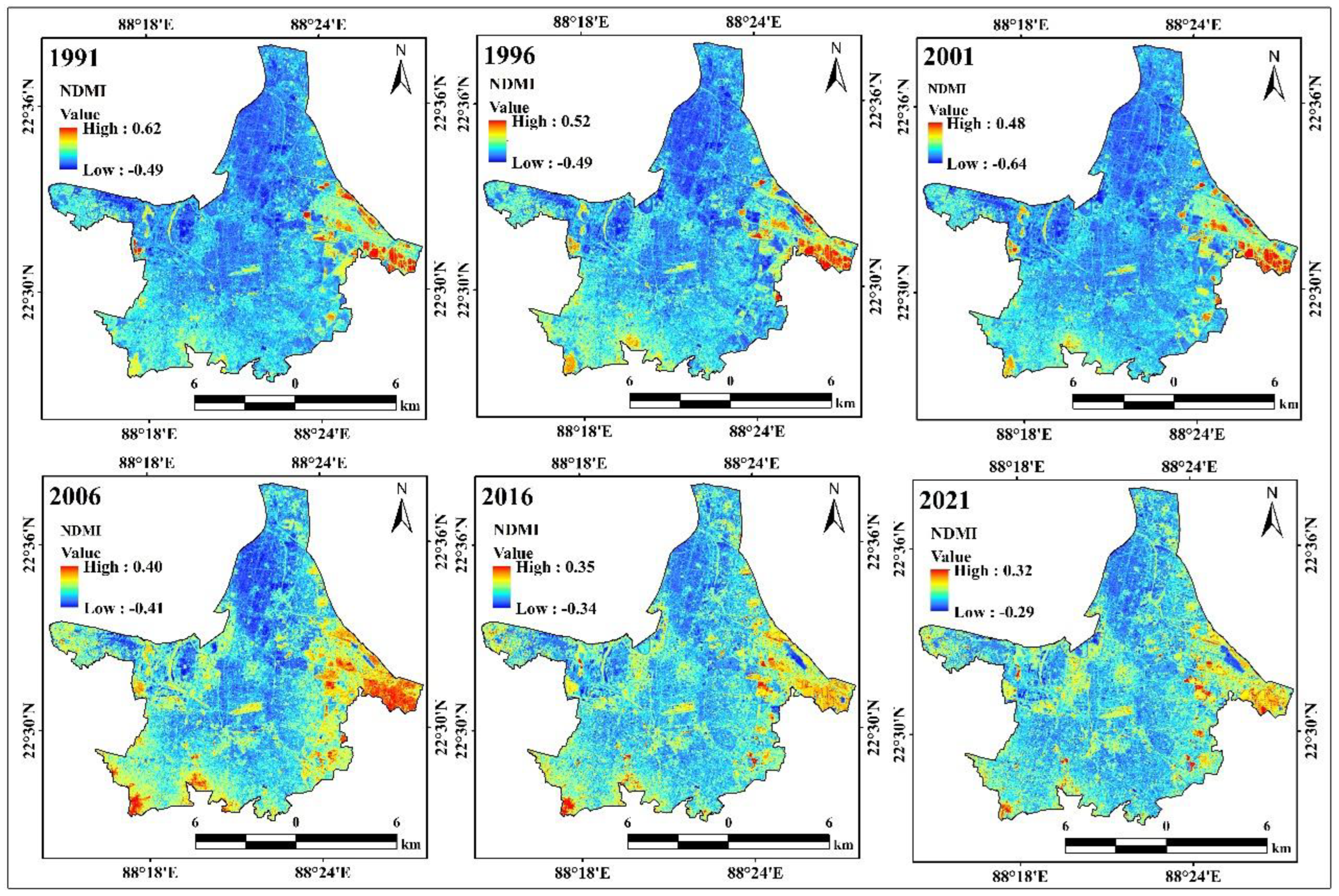
2.5.3. NDMI
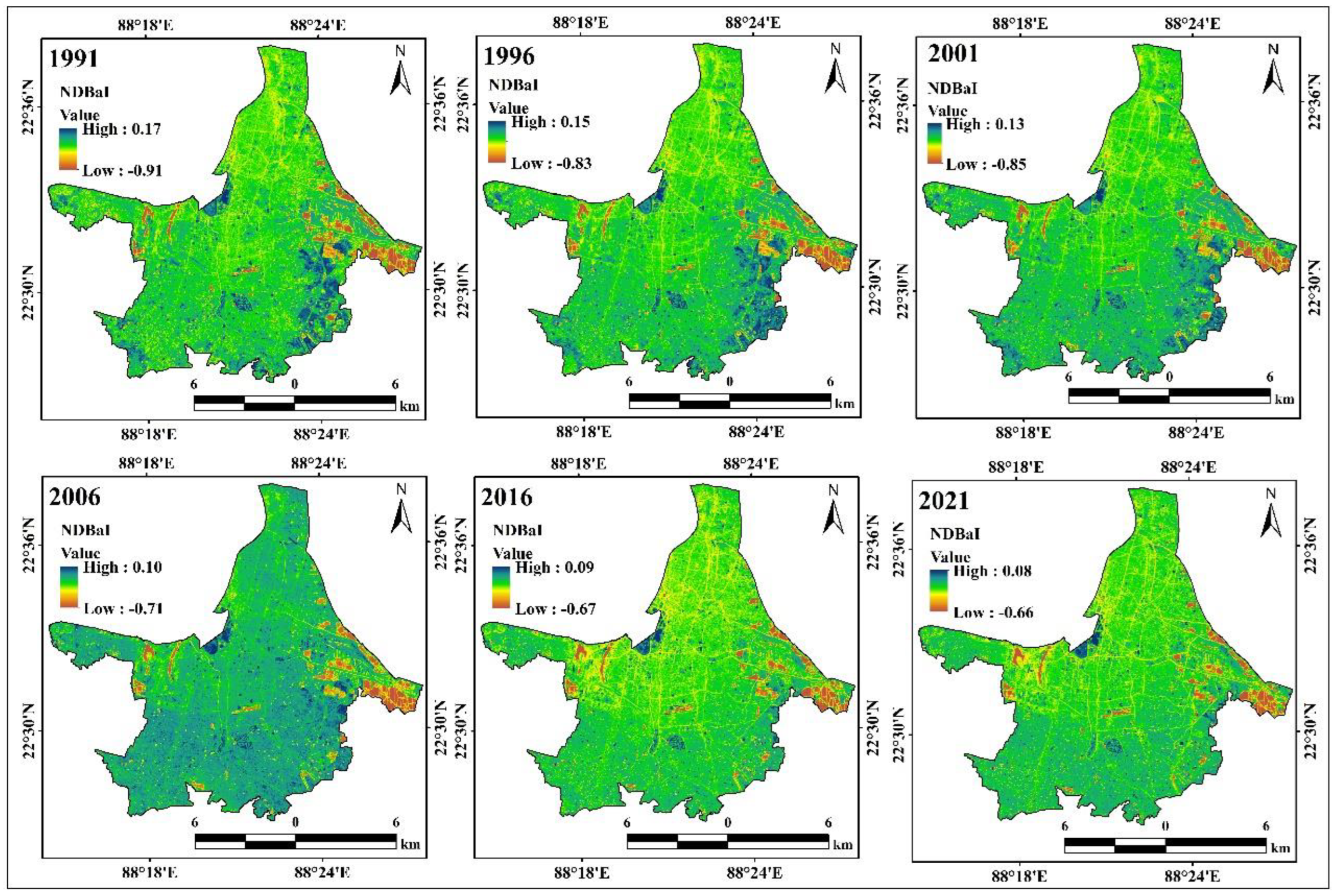
2.5.4. NDBal
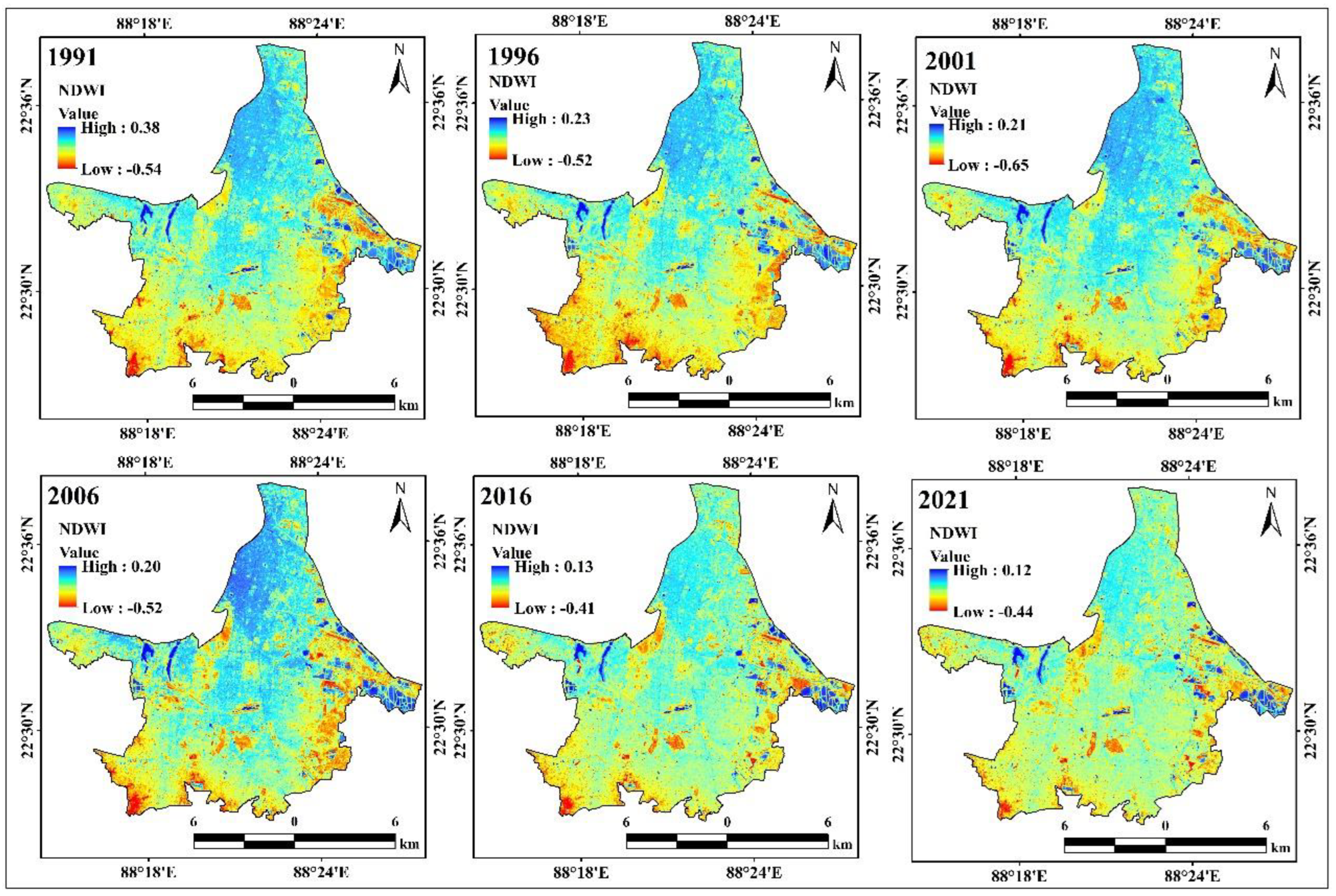
2.5.5. NDWI
2.6. LST Estimation
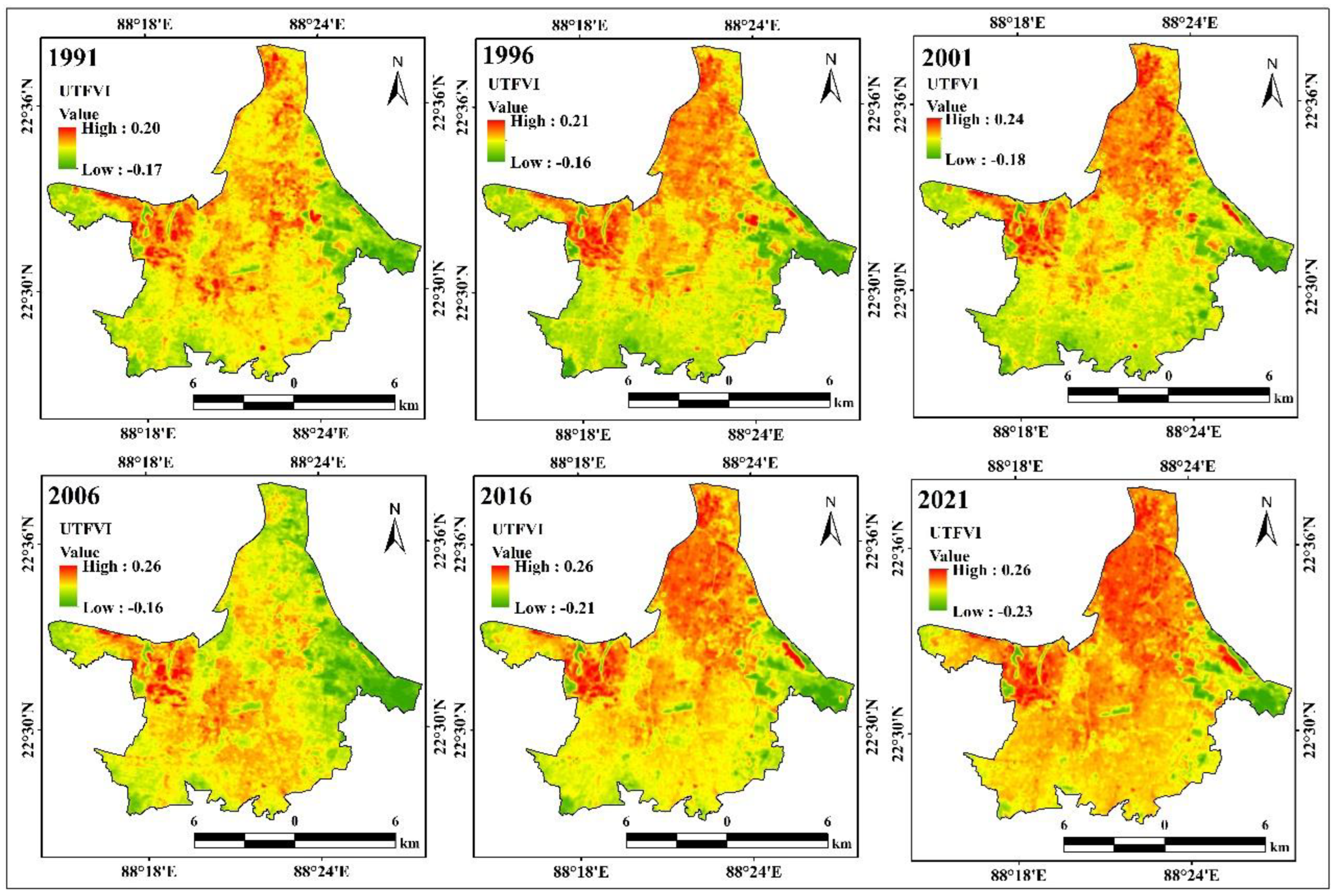
2.7. UTFVI
2.8. SUHI
3. Results and Discussion
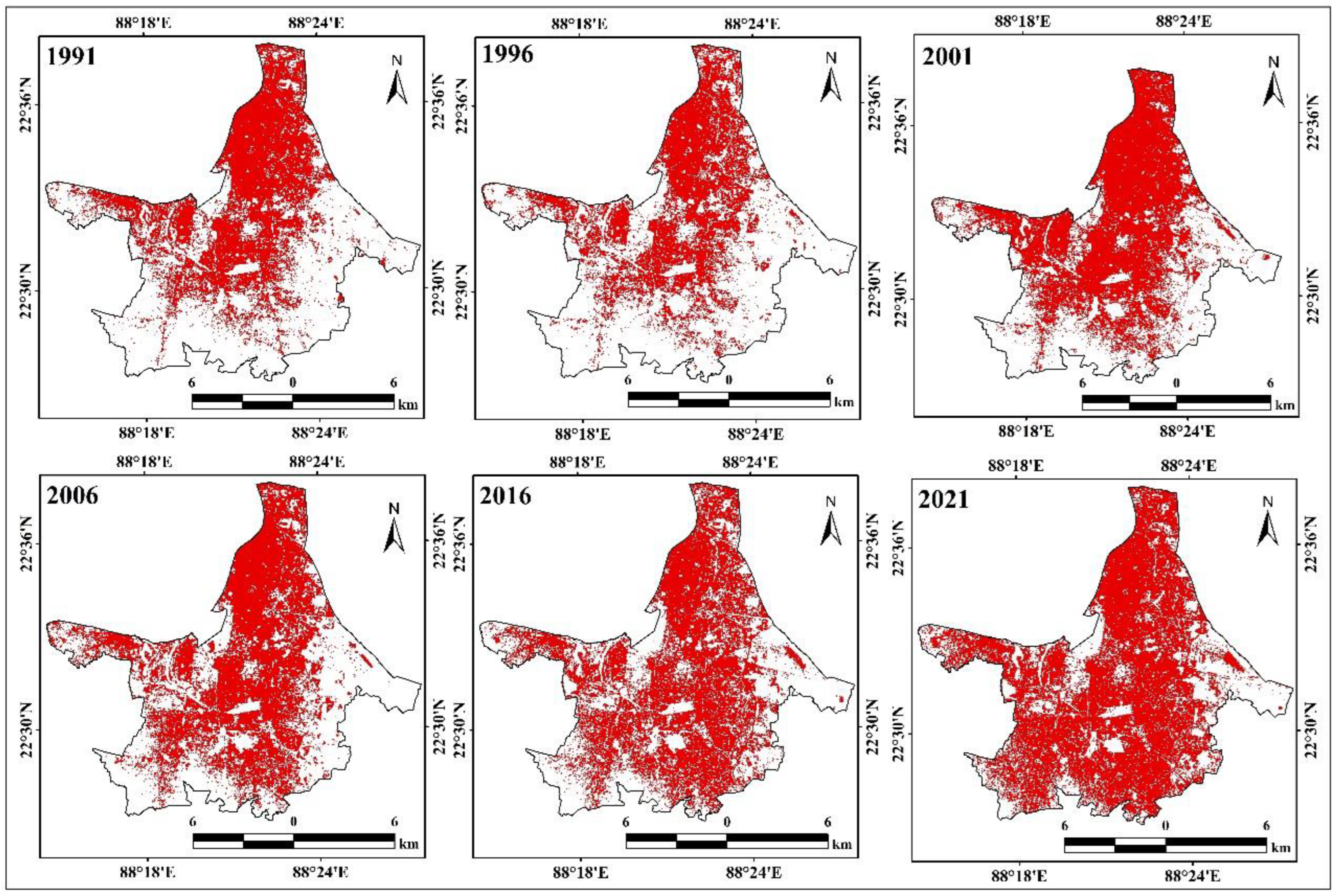
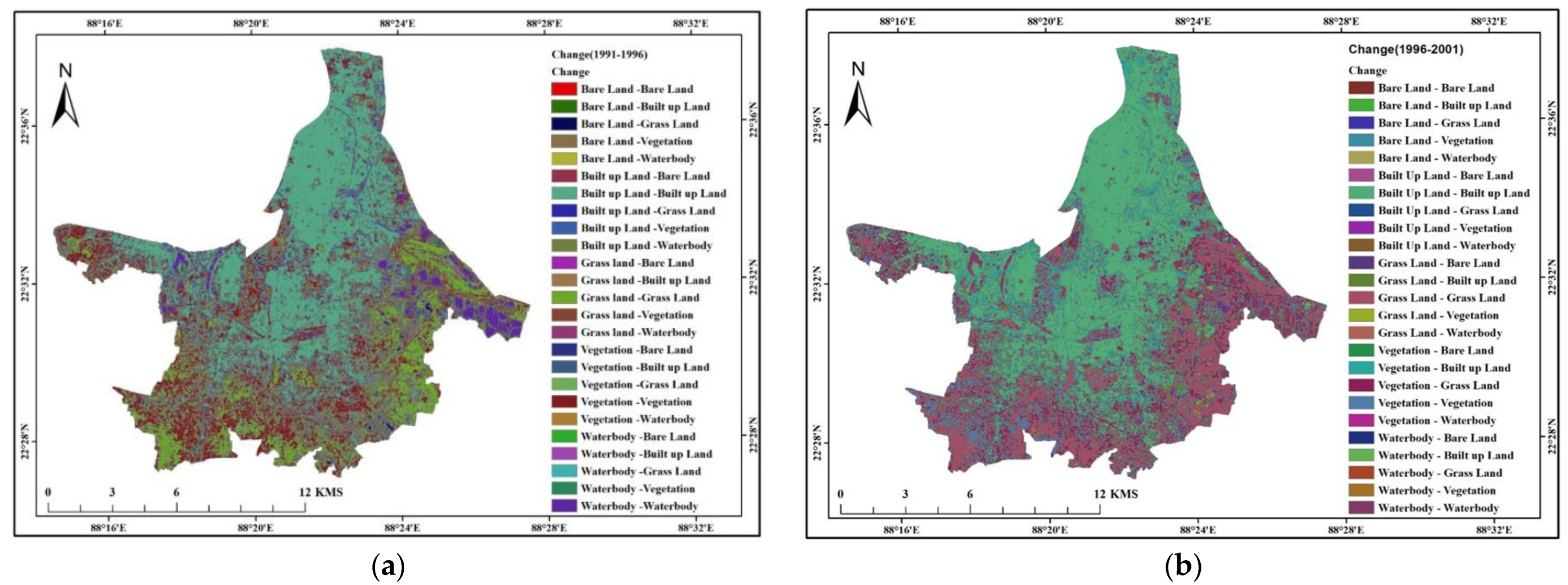
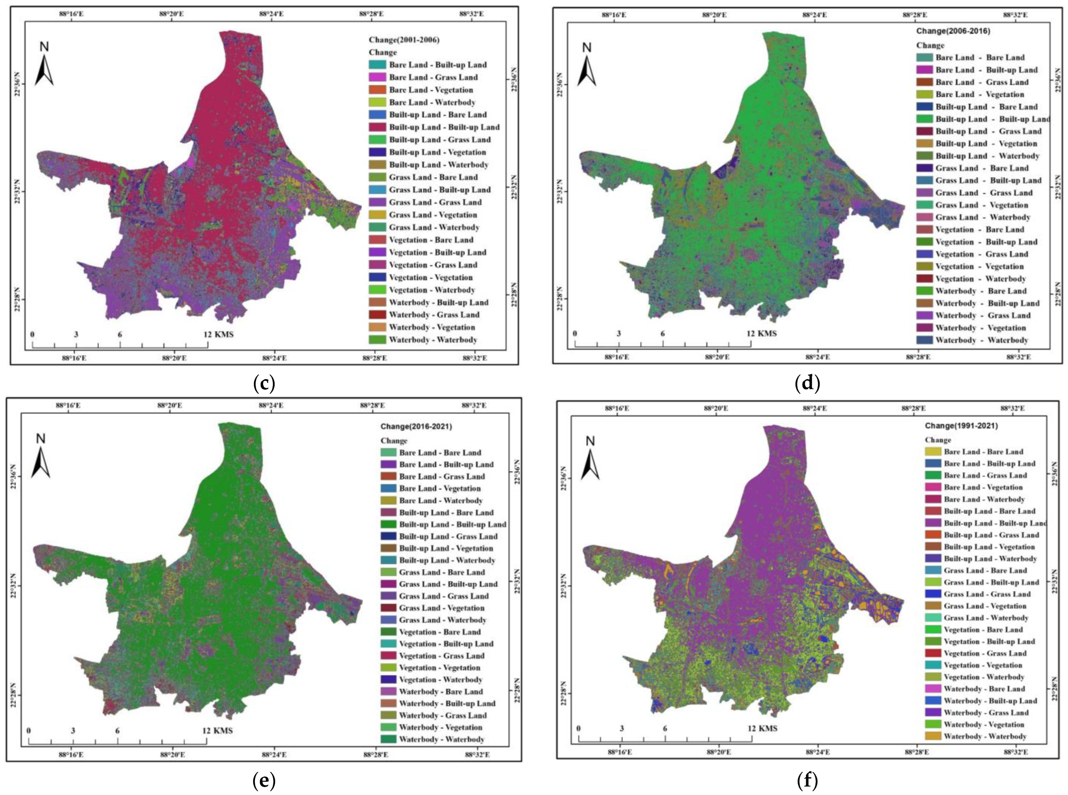
3.1. Areal Change of LULC
3.2. LST Variation
3.3. Geo-Spatial Indices
3.4. SUHI
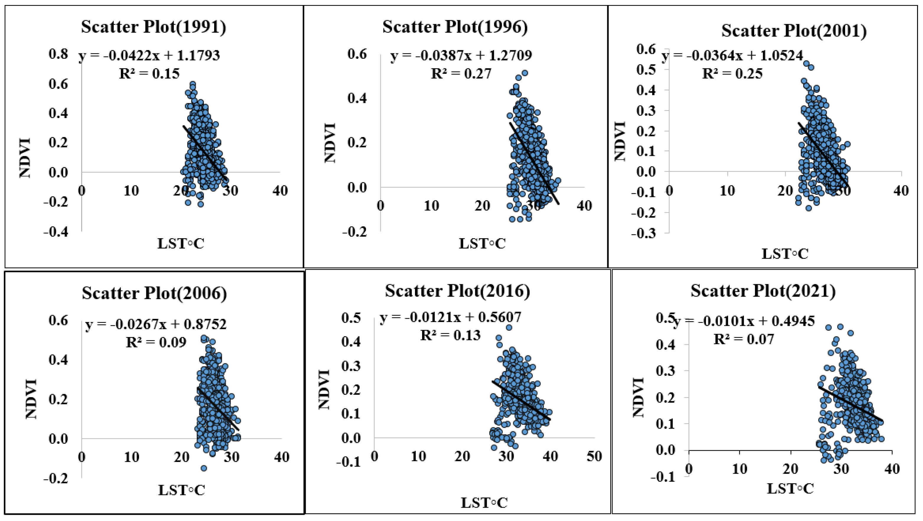
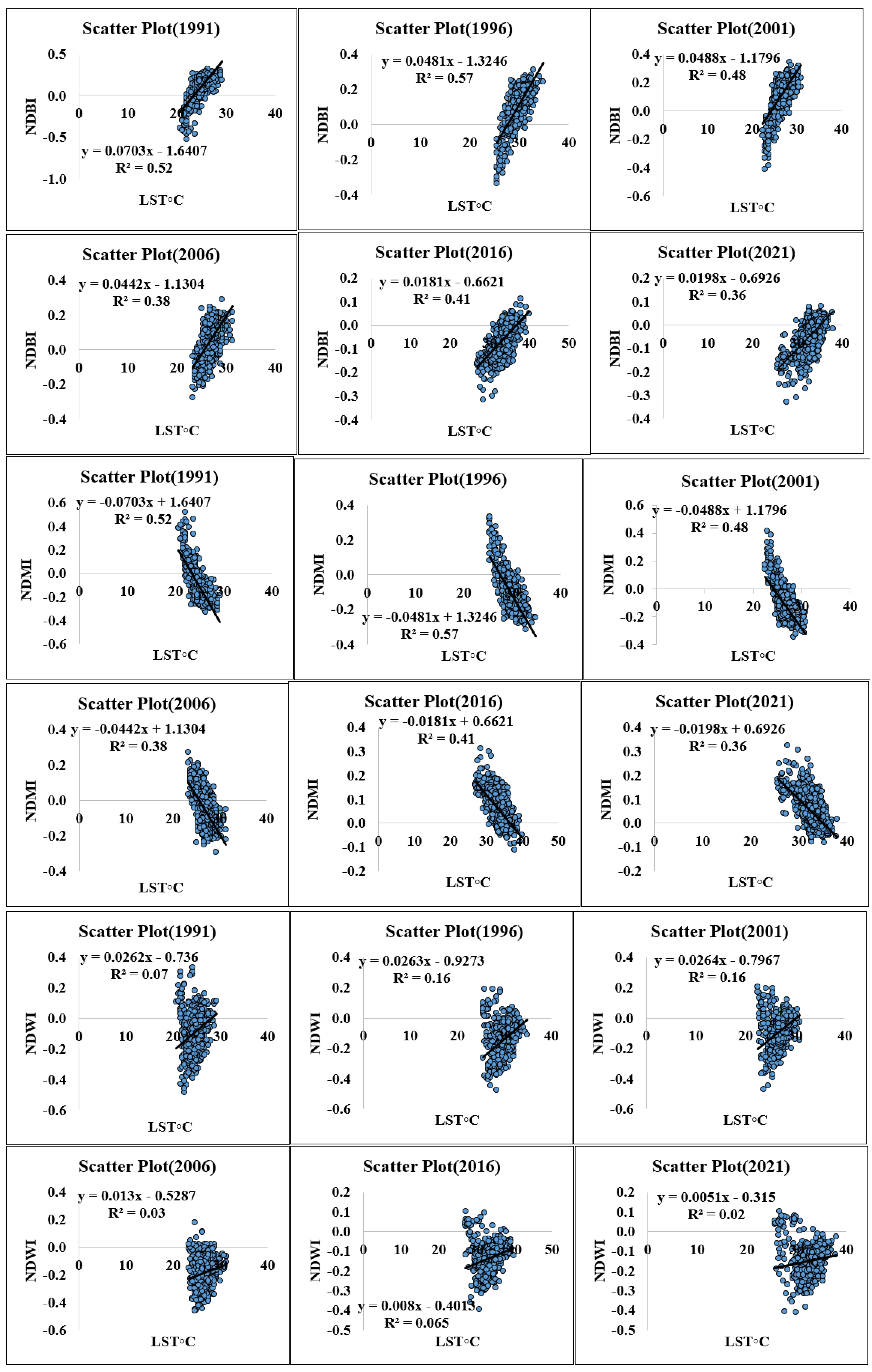
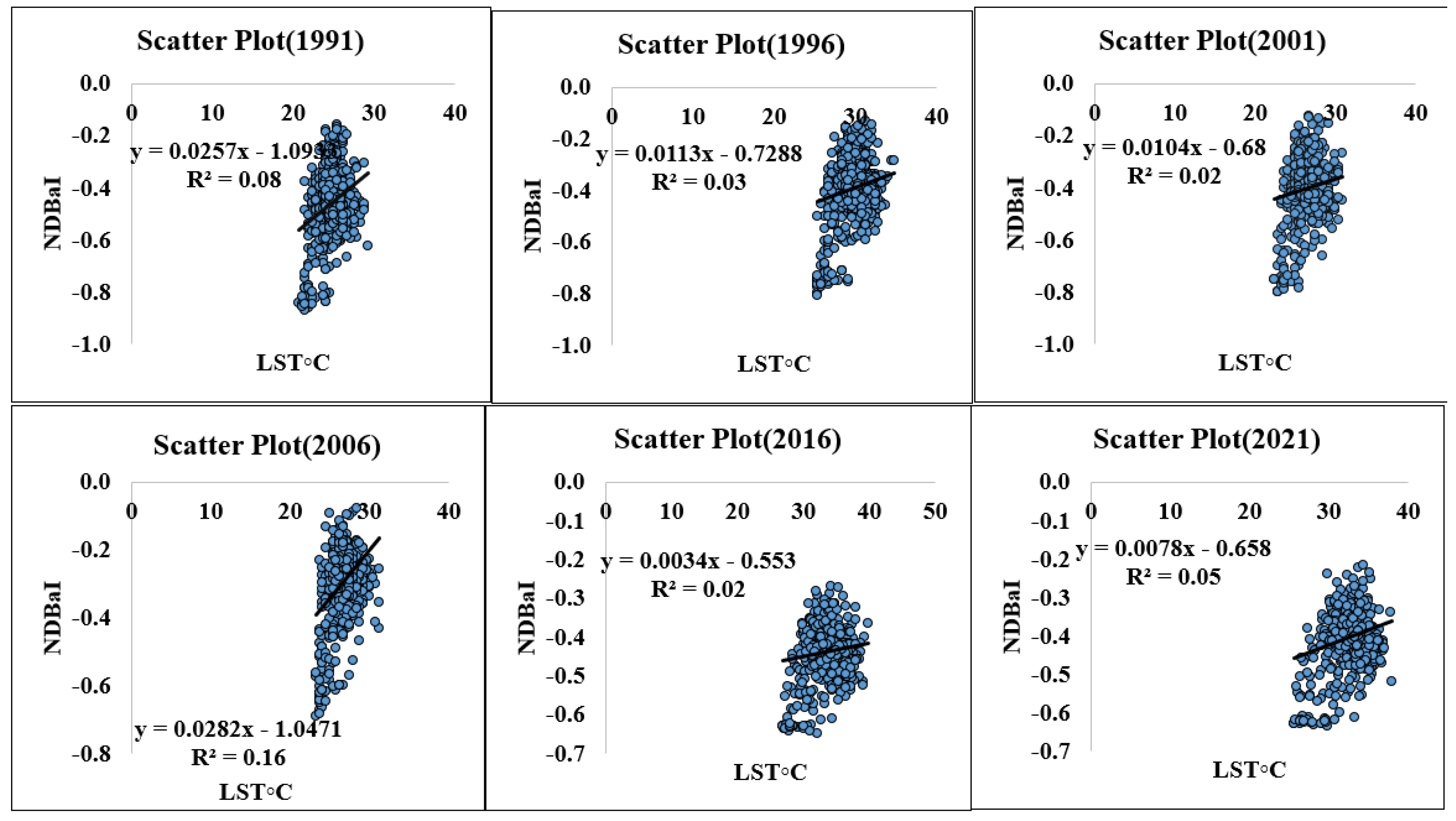
3.5. Correlation Analysis
3.6. Limitations and Recommendation
4. Conclusions
- The UHI and LULC results commend the significant strengthening in residential regions, similar to the temperature of the urbanized regions in the last three periods, as supplementary to added LULC features. The local thermal shape of the natural surroundings appears to have been impacted by the urbanization process, according to correlations found between LST and NDBI, NDVI, NDWI, NDMI, and NDBal.
- The significant positive link found between LST and NDBI suggests that rapid urban growth has directly impacted the region under investigation’s temperature conditions. Moreover, an inverse relationship between the decline in green space and the urban thermal field is suggested by the negative correlation between LST and NDVI.
- The primary regulating factor for SUHI and heat stress in Kolkata and the surrounding area, according to this study, is surface area. Policymakers, administrators, urban planners, and other interested parties can use this analysis for project management and planning that will reduce thermal variance and land modification over the KMC regions.
Author Contributions
Funding
Institutional Review Board Statement
Informed Consent Statement
Data Availability Statement
Acknowledgments
Conflicts of Interest
References
- Ishola, K.A.; Okogbue, E.C.; Adeyeri, O.E. Dynamics of Surface Urban Biophysical Compositions and Its Impact on Land Surface Thermal Field. Model. Earth Syst. Environ. 2016, 2, 1–20. [Google Scholar] [CrossRef]
- Atef, I.; Ahmed, W.; Abdel-Maguid, R.H. Modelling of Land Use Land Cover Changes Using Machine Learning and GIS Techniques: A Case Study in El-Fayoum Governorate, Egypt. Environ. Monit. Assess. 2023, 195, 637. [Google Scholar] [CrossRef] [PubMed]
- Armanuos, A.; Ahmed, K.; Sanusi Shiru, M.; Jamei, M. Impact of Increasing Pumping Discharge on Groundwater Level in the Nile Delta Aquifer, Egypt. Knowl.-Based Eng. Sci. 2021, 2, 13–23. [Google Scholar] [CrossRef]
- Zhang, S.; Omar, A.H.; Hashim, A.S.; Alam, T.; Khalifa, H.A.E.-W.; Elkotb, M.A. Enhancing Waste Management and Prediction of Water Quality in the Sustainable Urban Environment Using Optimized Algorithm of Least Square Support Vector Machine and Deep Learning Techniques. Urban Clim. 2023, 49, 101487. [Google Scholar] [CrossRef]
- Voogt, J.A.; Oke, T.R. Thermal Remote Sensing of Urban Climates. Remote Sens. Environ. 2003, 86, 370–384. [Google Scholar] [CrossRef]
- Lu, D.; Weng, Q. Use of Impervious Surface in Urban Land-Use Classification. Remote Sens. Environ. 2006, 102, 146–160. [Google Scholar] [CrossRef]
- Sarrat, C.; Lemonsu, A.; Masson, V.; Guedalia, D. Impact of Urban Heat Island on Regional Atmospheric Pollution. Atmos. Environ. 2006, 40, 1743–1758. [Google Scholar] [CrossRef]
- Abd Alraheem, E.; Jaber, N.A.; Jamei, M.; Tangang, F. Assessment of Future Meteorological Drought under Representative Concentration Pathways (RCP8. 5) Scenario: Case Study of Iraq. Knowl.-Based Eng. Sci. 2022, 3, 64–82. [Google Scholar]
- Mundia, C.N.; James, M.M. Dynamism of Land Use Changes on Surface Temperature in Kenya: A Case Study of Nairobi City. Int. J. Sci. Res. 2014, 3, 38–41. [Google Scholar]
- Avdan, U.; Jovanovska, G. Algorithm for Automated Mapping of Land Surface Temperature Using LANDSAT 8 Satellite Data. J. Sens. 2016, 2016, 1480307. [Google Scholar] [CrossRef]
- Cheruto, M.C.; Kauti, M.K.; Kisangau, D.P.; Kariuki, P.C. Assessment of Land Use and Land Cover Change Using GIS and Remote Sensing Techniques: A Case Study of Makueni County, Kenya. J. Remote. Sens. GIS 2016, 5, 1000175. [Google Scholar] [CrossRef]
- Meer, M.S.; Mishra, A.K. Land Use/Land Cover Changes over a District in Northern India Using Remote Sensing and GIS and Their Impact on Society and Environment. J. Geol. Soc. India 2020, 95, 179–182. [Google Scholar] [CrossRef]
- Estoque, R.C.; Murayama, Y.; Myint, S.W. Effects of Landscape Composition and Pattern on Land Surface Temperature: An Urban Heat Island Study in the Megacities of Southeast Asia. Sci. Total Environ. 2017, 577, 349–359. [Google Scholar] [CrossRef] [PubMed]
- Gohain, K.J.; Mohammad, P.; Goswami, A. Assessing the Impact of Land Use Land Cover Changes on Land Surface Temperature over Pune City, India. Quat. Int. 2021, 575, 259–269. [Google Scholar] [CrossRef]
- Mahmoud, A.A.; Mbengue, M.T.M.; Hussain, S.; Abdullahi, M.A.; Beddal, D.; Abba, S.I. Investigation for Flood Flow Quantification of Porous Asphalt with Different Surface and Subsurface Thickness. Knowl.-Based Eng. Sci. 2023, 4, 78–89. [Google Scholar]
- Zheng, B.; Myint, S.W.; Fan, C. Spatial Configuration of Anthropogenic Land Cover Impacts on Urban Warming. Landsc. Urban Plan. 2014, 130, 104–111. [Google Scholar] [CrossRef]
- Kumar, R.; Raj Gautam, H. Climate Change and Its Impact on Agricultural Productivity in India. J. Climatol. Weather Forecast. 2014, 2, 1000109. [Google Scholar] [CrossRef]
- Saleem, M.; Iqbal, J.; Shah, M.H. Non-Carcinogenic and Carcinogenic Health Risk Assessment of Selected Metals in Soil around a Natural Water Reservoir, Pakistan. Ecotoxicol. Environ. Saf. 2014, 108, 42–51. [Google Scholar] [CrossRef]
- Chakraborty, T.; Hsu, A.; Manya, D.; Sheriff, G. A Spatially Explicit Surface Urban Heat Island Database for the United States: Characterization, Uncertainties, and Possible Applications. ISPRS J. Photogramm. Remote Sens. 2020, 168, 74–88. [Google Scholar] [CrossRef]
- Shahmohamadi, P.; Che-Ani, A.I.; Etessam, I.; Maulud, K.N.A.; Tawil, N.M. Healthy Environment: The Need to Mitigate Urban Heat Island Effects on Human Health. Procedia Eng. 2011, 20, 61–70. [Google Scholar] [CrossRef]
- Gupta, K.; Kumar, P.; Pathan, S.K.; Sharma, K.P. Urban Neighborhood Green Index—A Measure of Green Spaces in Urban Areas. Landsc. Urban Plan. 2012, 105, 325–335. [Google Scholar] [CrossRef]
- Veettil, B.K.; Grondona, A.E.B. Vegetation Changes and Formation of Small-Scale Urban Heat Islands in Three Populated Districts of Kerala State, India. Acta Geophys. 2018, 66, 1063–1072. [Google Scholar] [CrossRef]
- Hashim, B.M.; Sultan, M.A.; Attyia, M.N.; Al Maliki, A.A.; Al-Ansari, N. Change Detection and Impact of Climate Changes to Iraqi Southern Marshes Using Landsat 2 Mss, Landsat 8 Oli and Sentinel 2 Msi Data and Gis Applications. Appl. Sci. 2019, 9, 2016. [Google Scholar] [CrossRef]
- Jamei, M.; Ali, M.; Jun, C.; Bateni, S.M.; Karbasi, M.; Farooque, A.A.; Yaseen, Z.M. Multi-Step Ahead Hourly Forecasting of Air Quality Indices in Australia: Application of an Optimal Time-Varying Decomposition-Based Ensemble Deep Learning Algorithm. Atmos. Pollut. Res. 2023, 14, 101752. [Google Scholar] [CrossRef]
- Yu, X.; Guo, X.; Wu, Z. Land Surface Temperature Retrieval from Landsat 8 TIRS—Comparison between Radiative Transfer Equation-Based Method, Split Window Algorithm and Single Channel Method. Remote Sens. 2014, 6, 9829–9852. [Google Scholar] [CrossRef]
- Ke, Y.; Im, J.; Lee, J.; Gong, H.; Ryu, Y. Characteristics of Landsat 8 OLI-Derived NDVI by Comparison with Multiple Satellite Sensors and In-Situ Observations. Remote Sens. Environ. 2015, 164, 298–313. [Google Scholar] [CrossRef]
- Sekertekin, A.; Bonafoni, S. Land Surface Temperature Retrieval from Landsat 5, 7, and 8 over Rural Areas: Assessment of Different Retrieval Algorithms and Emissivity Models and Toolbox Implementation. Remote Sens. 2020, 12, 294. [Google Scholar] [CrossRef]
- Carlson, T. An Overview of the “Triangle Method” for Estimating Surface Evapotranspiration and Soil Moisture from Satellite Imagery. Sensors 2007, 7, 1612–1629. [Google Scholar] [CrossRef]
- Omran, E.-S.E. Detection of Land-Use and Surface Temperature Change at Different Resolutions. J. Geogr. Inf. Syst. 2012, 4, 189–203. [Google Scholar] [CrossRef]
- Orhan, O.; Ekercin, S.; Dadaser-Celik, F. Use of Landsat Land Surface Temperature and Vegetation Indices for Monitoring Drought in the Salt Lake Basin Area, Turkey. Sci. World J. 2014, 2014, 142939. [Google Scholar] [CrossRef]
- Berwal, S.; Kumar, D.; Pandey, A.K.; Singh, V.P.; Kumar, R.; Kumar, K. Dynamics of Thermal Inertia over Highly Urban City: A Case Study of Delhi. In Remote Sensing Technologies and Applications in Urban Environments; SPIE: Bellingham, WA, USA, 2016; Volume 10008, pp. 108–114. [Google Scholar]
- Kayet, N.; Pathak, K.; Chakrabarty, A.; Sahoo, S. Spatial Impact of Land Use/Land Cover Change on Surface Temperature Distribution in Saranda Forest, Jharkhand. Model. Earth Syst. Environ. 2016, 2, 127. [Google Scholar] [CrossRef]
- Jensen Mausel, P.; Dias, N.; Gonser, R.; Yang, C.; Everitt, J.; Fletcher, R. Spectral Analysis of Coastal Vegetation and Land Cover Using AISA+ Hyperspectral Data. Geocarto Int. 2007, 22, 17–28. [Google Scholar] [CrossRef]
- Cohen, J. Weighted Kappa: Nominal Scale Agreement Provision for Scaled Disagreement or Partial Credit. Psychol. Bull. 1968, 70, 213. [Google Scholar] [CrossRef] [PubMed]
- Zoungrana, B.J.B.; Conrad, C.; Thiel, M.; Amekudzi, L.K.; Da, E.D. MODIS NDVI Trends and Fractional Land Cover Change for Improved Assessments of Vegetation Degradation in Burkina Faso, West Africa. J. Arid Environ. 2018, 153, 66–75. [Google Scholar] [CrossRef]
- Li, Q.; Zhang, T.; Yu, Y. Using Cloud Computing to Process Intensive Floating Car Data for Urban Traffic Surveillance. Int. J. Geogr. Inf. Sci. 2011, 25, 1303–1322. [Google Scholar] [CrossRef]
- Jin, Z.; Zhang, L.; Lv, J.; Sun, X. The Application of Geostatistical Analysis and Receptor Model for the Spatial Distribution and Sources of Potentially Toxic Elements in Soils. Environ. Geochem. Health 2021, 43, 407–421. [Google Scholar] [CrossRef] [PubMed]
- Sobrino, J.A.; Raissouni, N.; Li, Z.-L. A Comparative Study of Land Surface Emissivity Retrieval from NOAA Data. Remote Sens. Environ. 2001, 75, 256–266. [Google Scholar] [CrossRef]
- Guha, S.; Govil, H.; Dey, A.; Gill, N. Analytical Study of Land Surface Temperature with NDVI and NDBI Using Landsat 8 OLI and TIRS Data in Florence and Naples City, Italy. Eur. J. Remote Sens. 2018, 51, 667–678. [Google Scholar] [CrossRef]
- Singh, P.; Kikon, N.; Verma, P. Impact of Land Use Change and Urbanization on Urban Heat Island in Lucknow City, Central India. A Remote Sensing Based Estimate. Sustain. Cities Soc. 2017, 32, 100–114. [Google Scholar] [CrossRef]
- Kedia, S.; Bhakare, S.P.; Dwivedi, A.K.; Islam, S.; Kaginalkar, A. Estimates of Change in Surface Meteorology and Urban Heat Island over Northwest India: Impact of Urbanization. Urban Clim. 2021, 36, 100782. [Google Scholar] [CrossRef]
- Chandler, T.J. Urban Climatology and Urban Planning. Geogr. J. 1976, 142, 57. [Google Scholar] [CrossRef]
- Estoque, R.C.; Murayama, Y. Monitoring Surface Urban Heat Island Formation in a Tropical Mountain City Using Landsat Data (1987–2015). ISPRS J. Photogramm. Remote Sens. 2017, 133, 18–29. [Google Scholar] [CrossRef]
- Zhao, H.; Chen, X. Use of Normalized Difference Bareness Index in Quickly Mapping Bare Areas from TM/ETM+. In Proceedings of the International Geoscience and Remote Sensing Symposium, Seoul, Republic of Korea, 29 July 2005; Volume 3, p. 1666. [Google Scholar]
- Guha, S.; Govil, H.; Besoya, M. An Investigation on Seasonal Variability between LST and NDWI in an Urban Environment Using Landsat Satellite Data. Geomat. Nat. Hazards Risk 2020, 11, 1319–1345. [Google Scholar] [CrossRef]
- Sobrino, J.A.; Jiménez-Muñoz, J.C.; Paolini, L. Land Surface Temperature Retrieval from LANDSAT TM 5. Remote Sens. Environ. 2004, 90, 434–440. [Google Scholar] [CrossRef]
- Scarano, M.; Sobrino, J.A. On the Relationship between the Sky View Factor and the Land Surface Temperature Derived by Landsat-8 Images in Bari, Italy. Int. J. Remote Sens. 2015, 36, 4820–4835. [Google Scholar] [CrossRef]
- Mirzaei, P.A.; Haghighat, F. Approaches to Study Urban Heat Island—Abilities and Limitations. Build. Environ. 2010, 45, 2192–2201. [Google Scholar] [CrossRef]
- Abir, F.A.; Ahmmed, S.; Sarker, S.H.; Fahim, A.U. Thermal and Ecological Assessment Based on Land Surface Temperature and Quantifying Multivariate Controlling Factors in Bogura, Bangladesh. Heliyon 2021, 7, e08012. [Google Scholar] [CrossRef] [PubMed]
- Ray, R.; Das, A.; Hasan, M.S.U.; Aldrees, A.; Islam, S.; Khan, M.A.; Lama, G.F.C. Quantitative Analysis of Land Use and Land Cover Dynamics Using Geoinformatics Techniques: A Case Study on Kolkata Metropolitan Development Authority (KMDA) in West Bengal, India. Remote Sens. 2023, 15, 959. [Google Scholar] [CrossRef]
- Sharma, R.; Chakraborty, A.; Joshi, P.K. Geospatial Quantification and Analysis of Environmental Changes in Urbanizing City of Kolkata (India). Environ. Monit. Assess. 2015, 187, 4206. [Google Scholar] [CrossRef]
- Hasnine, M.; Rukhsana. Spatial and Temporal Analysis of Land Use and Land Cover Change in and around Kolkata City, India, Using Geospatial Techniques. J. Indian Soc. Remote Sens. 2023, 51, 1037–1056. [Google Scholar] [CrossRef]
- Das, P.; Vamsi, K.S.; Zhenke, Z. Decadal Variation of the Land Surface Temperatures (LST) and Urban Heat Island (UHI) over Kolkata City Projected Using MODIS and ERA-Interim DataSets. Aerosol Sci. Eng. 2020, 4, 200–209. [Google Scholar] [CrossRef]
- Biswas, S.; Ghosh, S. Estimation of Land Surface Temperature in Response to Land Use/Land Cover Transformation in Kolkata City and Its Suburban Area, India. Int. J. Urban Sci. 2022, 26, 604–631. [Google Scholar] [CrossRef]
- Ali, M.B.; Jamal, S.; Ahmad, M.; Saqib, M. Unriddle the Complex Associations among Urban Green Cover, Built-up Index, and Surface Temperature Using Geospatial Approach: A Micro-Level Study of Kolkata Municipal Corporation for Sustainable City. Theor. Appl. Climatol. 2024, 1–22. [Google Scholar] [CrossRef]
- Lu, L.; Fu, P.; Dewan, A.; Li, Q. Contrasting Determinants of Land Surface Temperature in Three Megacities: Implications to Cool Tropical Metropolitan Regions. Sustain. Cities Soc. 2023, 92, 104505. [Google Scholar] [CrossRef]
- Bhowmick, D.; Mukherjee, K.; Dash, P.; Mondal, R. Use of “Local Climate Zones” for Detecting Urban Heat Island: A Case Study of Kolkata Metropolitan Area, India. In IOP Conference Series: Earth and Environmental Science, Proceedings of the International Conference on Geospatial Science for Digital Earth Observation (GSDEO-2021), Online, 26–27 March 2021; IOP Publishing: Bristol, UK, 2023; Volume 1164, p. 12007. [Google Scholar]
- Khorat, S.; Das, D.; Khatun, R.; Aziz, S.M.; Anand, P.; Khan, A.; Santamouris, M.; Niyogi, D. Cool Roof Strategies for Urban Thermal Resilience to Extreme Heatwaves in Tropical Cities. Energy Build. 2024, 302, 113751. [Google Scholar] [CrossRef]
- Sharma, R.; Pradhan, L.; Kumari, M.; Bhattacharya, P. Assessing Urban Heat Islands and Thermal Comfort in Noida City Using Geospatial Technology. Urban Clim. 2021, 35, 100751. [Google Scholar] [CrossRef]
- Ceccato, P.; Flasse, S.; Tarantola, S.; Jacquemoud, S.; Grégoire, J.-M. Detecting Vegetation Leaf Water Content Using Reflectance in the Optical Domain. Remote Sens. Environ. 2001, 77, 22–33. [Google Scholar] [CrossRef]
- Yao, X.; Yu, K.; Zeng, X.; Lin, Y.; Ye, B.; Shen, X.; Liu, J. How Can Urban Parks Be Planned to Mitigate Urban Heat Island Effect in “Furnace Cities”? An Accumulation Perspective. J. Clean. Prod. 2022, 330, 129852. [Google Scholar] [CrossRef]
- Alexander, C. Normalised Difference Spectral Indices and Urban Land Cover as Indicators of Land Surface Temperature (LST). Int. J. Appl. Earth Obs. Geoinf. 2020, 86, 102013. [Google Scholar] [CrossRef]
- Mohamed, A.H.; Adwan, I.A.I.; Ahmeda, A.G.F.; Hrtemih, H.; Al-MSari, H. Identification of Affecting Factors on the Travel Time Reliability for Bus Transportation. Knowl.-Based Eng. Sci. 2021, 2, 19–30. [Google Scholar] [CrossRef]


| Satellite | Sensor | Date of Acquisition | Path/Row | Website |
|---|---|---|---|---|
| Landsat 5 | TM | 6 March 1991 | 138/044 | https://earthexplorer.usgs.gov/, accessed on 12 March 2023 |
| 20 March 1996 | ||||
| 17 March 2001 | ||||
| 19 June 2006 | ||||
| Landsat 8 | OLI/TIRS | 11 April 2016 | ||
| 25 April 2021 |
| Built-up land | Residential area, commercial area, industrial area, transportation, roads, and construction area. |
| Vegetation | Evergreen forest, deciduous Forest Land, Mixed Forest Land, Shrub/degraded vegetation. |
| Water Bodies | River, Ponds, lakes, and open water bodies. |
| Bare land | These types of classes are mainly playgrounds, open area, and many others. |
| Grass Land | Many types of trees, Grass area, open vegetated area |
| SL. No | Value of K | Strength of Agreement |
|---|---|---|
| 1 | <0.20 | Poor |
| 2 | 0.21–0.40 | Fair |
| 3 | 0.41–0.60 | Moderate |
| 4 | 0.61–0.80 | Good |
| 5 | 0.81–1.00 | Very Good |
| Class Name | Area in Ha | |||||
|---|---|---|---|---|---|---|
| 1991 | 1996 | 2001 | 2006 | 2016 | 2021 | |
| Water body | 875.43 | 614.43 | 523.89 | 682.56 | 785.97 | 441.27 |
| Vegetation | 4050.27 | 6591.51 | 1374.03 | 2899.44 | 4837.77 | 2695.41 |
| Grass Land | 5127.93 | 4198.95 | 5928.21 | 5561.55 | 1694.25 | 2841.03 |
| Built-up Land | 7721.55 | 6978.15 | 10,241.73 | 9406.98 | 10071 | 12,450.78 |
| Bare Land | 779.04 | 171.18 | 486.36 | 3.69 | 1165.23 | 125.73 |
| Class Name | Area in Percentage (%) | |||||
| 1991 | 1996 | 2001 | 2006 | 2016 | 2021 | |
| Water body | 4.71 | 3.31 | 2.82 | 3.67 | 4.23 | 2.37 |
| Vegetation | 21.82 | 35.52 | 7.4 | 15.62 | 26.07 | 14.52 |
| Grass Land | 27.63 | 22.63 | 31.95 | 29.97 | 9.13 | 15.31 |
| Built-up Land | 41.61 | 37.6 | 55.19 | 50.69 | 54.27 | 67.1 |
| Bare Land | 4.19 | 0.92 | 2.62 | 0.01 | 6.28 | 0.67 |
| Class Name | Area Increased/Decreased (Ha) | |||||
|---|---|---|---|---|---|---|
| (1991–1996) | (1996–2001) | (2001–2006) | (2006–2016) | (2016–2021) | (1991–2021) | |
| Water body | −261 | −90.54 | 158.67 | 103.41 | −344.7 | −434.16 |
| Vegetation | 2541.24 | −5217.48 | 1525.41 | 1938.33 | −2142.36 | −1354.86 |
| Grass Land | −928.98 | 1729.26 | −366.66 | −3867.3 | 1146.78 | −2286.9 |
| Built-up Land | −743.4 | 3263.58 | −834.75 | 664.02 | 2379.78 | 4729.23 |
| Bare Land | −607.86 | 315.18 | −482.67 | 1161.54 | −1039.5 | −653.31 |
Disclaimer/Publisher’s Note: The statements, opinions and data contained in all publications are solely those of the individual author(s) and contributor(s) and not of MDPI and/or the editor(s). MDPI and/or the editor(s) disclaim responsibility for any injury to people or property resulting from any ideas, methods, instructions or products referred to in the content. |
© 2024 by the authors. Licensee MDPI, Basel, Switzerland. This article is an open access article distributed under the terms and conditions of the Creative Commons Attribution (CC BY) license (https://creativecommons.org/licenses/by/4.0/).
Share and Cite
Gorai, N.; Bandyopadhyay, J.; Halder, B.; Ahmed, M.F.; Molla, A.H.; Lei, T.M.T. Spatio-Temporal Variation in Landforms and Surface Urban Heat Island in Riverine Megacity. Sustainability 2024, 16, 3383. https://doi.org/10.3390/su16083383
Gorai N, Bandyopadhyay J, Halder B, Ahmed MF, Molla AH, Lei TMT. Spatio-Temporal Variation in Landforms and Surface Urban Heat Island in Riverine Megacity. Sustainability. 2024; 16(8):3383. https://doi.org/10.3390/su16083383
Chicago/Turabian StyleGorai, Namita, Jatisankar Bandyopadhyay, Bijay Halder, Minhaz Farid Ahmed, Altaf Hossain Molla, and Thomas M. T. Lei. 2024. "Spatio-Temporal Variation in Landforms and Surface Urban Heat Island in Riverine Megacity" Sustainability 16, no. 8: 3383. https://doi.org/10.3390/su16083383