Abstract
Dockless bike-sharing (DBS) plays a crucial role in solving the “last-mile” problem for metro trips. However, bike–metro transfer usage varies by time and transfer flows. This study explores the nonlinear relationship between the built environment and bike–metro transfer in Shenzhen, considering different times and transfer flows while incorporating spatial dependence to improve model accuracy. We integrated smart card records and DBS data to identify transfer trips and categorized them into four types: morning access, morning egress, evening access, and evening egress. Using random forest and gradient boosting decision tree models, we found that (1) introducing spatial lag terms significantly improved model accuracy, indicating the importance of spatial dependence in bike–metro transfer; (2) the built environment’s impact on bike–metro transfer exhibited distinct nonlinear patterns, particularly for bus stop density, house prices, commercial points of interest (POI), and cultural POI, varying by time and transfer flow; (3) SHAP value analysis further revealed the influence of urban spatial structure on bike–metro transfer, with residential and employment areas displaying different transfer patterns by time and transfer flow. Our findings underscore the importance of considering both built environment factors and spatial dependence in urban transportation planning to achieve sustainable and efficient transportation systems.
1. Introduction
As urbanization accelerates, issues such as traffic congestion, air pollution, and prolonged commute times have become more severe, especially during peak hours. These problems place immense pressure on urban transportation systems and negatively affect the quality of life for residents. Governments have promoted transit-oriented development, particularly the expansion of metro systems, to address these challenges [1]. While metros alleviate traffic pressure in city centers, the “last-mile” issue remains unresolved. Dockless bike-sharing (DBS), as a valuable supplement to metro transit, has emerged as an effective solution to this problem [2]. Consequently, maximizing the integration of DBS and metro transfers through urban planning has become crucial for improving transportation efficiency.
The influence of the built environment on bike–metro transfer varies significantly across different times and transfer flows [3]. During peak hours, trip demand is highly concentrated in specific directions. In the morning peak, most trips are from residential areas to work areas, while the evening peak shows the reverse pattern, with more people returning to residential areas from work [4]. These directional flows generate distinct demand patterns that influence the built environment’s effect on bike–metro transfer [5]. Analyzing peak-period metro transfer is essential for addressing these time-specific challenges and ensuring that the system meets peak demand and maintains efficiency.
In addition, the relationship between the built environment and bike–metro transfer is inherently complex due to multi-level interactions among urban factors [6]. On the one hand, the impact of built environment elements on bike–metro transfer may not follow a simple proportional or linear pattern [7]. For example, increasing bus stop density can enhance transfer trips up to a certain threshold, but beyond that point, additional stops may cause congestion and reduce efficiency [8]. On the other hand, urban space forms a continuous, highly interconnected system [9]. Spatial dependence indicates that characteristics and phenomena at one location are influenced by adjacent areas [10]. Within metro transfer contexts, a station’s accessibility and attractiveness can influence usage at nearby stations. Without considering spatial dependence, models may miss neighboring effects and regional interactions [11]. We find that incorporating spatial dependence to explore nonlinear relationships between the built environment and bike–metro transfer facilitates a more accurate understanding of urban commuting complexity [12].
In this context, this study aims to reveal the nonlinear relationship between the built environment and bike–metro transfer, integrating spatial dependence with machine learning models. Specifically, the main research questions include the following: (1) how to comprehensively analyze bike–metro transfer characteristics under different peak periods and transfer flow conditions using large-scale individual-level chain data; (2) how spatial dependence influences bike–metro transfer and affects model performance; and (3) how built environment elements produce nonlinear effects on bike–metro transfer at various times and transfer flows. We consider addressing these issues crucial, as a deeper understanding of the driving factors and spatial interactions in bike–metro transfer can offer scientific support to urban transportation planners, optimize the integration of public transit with dockless bicycles, enhance efficiency, reduce congestion, and promote urban sustainability.
2. Literature Review
DBS has become a widely recognized solution for addressing the “last-mile” problem, particularly when integrated with metro systems. However, most existing studies rely on small samples, such as survey data [13] or aggregated data near metro stations [14], which lack complete individual-level trip chain data, limiting their practical application in urban planning [15]. Many studies assume that all bike trips near metro stations are transferred, potentially overestimating actual bike–metro transfer counts [7,16]. Early research often focused on overall bike–metro transfer characteristics, such as daily trip volumes, total transfer trips in specific areas, or young people’s use of bike–metro transfers [17]. As research has progressed, scholars have increasingly recognized that transfer trips vary significantly across different times and transfer flows [18]. This shows that bike–metro transfer is not a static phenomenon but a process driven by spatial and temporal factors. For instance, studies have shown that the duration and distance of transfer trips entering and exiting stations are similar [14]. Additionally, PM2.5 emissions are positively correlated with cycling during peak hours [19]. However, most studies focus on single spatial or temporal dimensions and do not explore the interactions between different times and transfer flows.
Regarding the built environment’s influence on transfer, researchers typically adopt the “5D principle”, which includes density, diversity, design, distance to transit, and destination accessibility [20,21]. For example, existing studies [22] have found that high population and employment densities significantly promote cycling, while other research [23] has noted that different land use densities have varying effects on bike–metro transfer trips. Further studies [24] have emphasized the importance of streetscape features, such as the green view index and sky view index, in influencing cycling trips. However, most studies use traditional linear models [25], which cannot fully capture complex nonlinear and spatial relations.
With advancements in research methods, scholars have begun to acknowledge the multiple interactions between the built environment and bike–metro transfer, particularly regarding spatial dependence [26]. Although some studies have introduced spatial econometric models, such as spatial lag models and spatial Durbin models [27], traditional spatial models capture only linear effects. They are inadequate for revealing nonlinear interactions [28]. In recent years, researchers have applied advanced models, such as random forest (RF), gradient boosting decision trees (GBDT), extreme gradient boosting (XGboost) [29], and categorical boosting (Catboost) [30] to analyze nonlinear relationships between the built environment and various spatiotemporal behaviors [31,32,33]. However, these models often overlook spatial dependencies [34], which are crucial for understanding interactions between neighboring areas. In addition, SHAP (Shapley additive explanations) quantifies each variable’s contribution [35] and shows promise in fields such as urban crime analysis and housing price prediction [26,36], but remains underexplored in the context of bike–metro transfer.
This study addresses two key gaps: (1) the lack of large-scale individual-level trip chain data for analyzing bike–metro transfer, with existing studies mainly focused on aggregate bike–metro transfer characteristics and overlooking the interactions between different times and transfer flows; (2) the limitation of conventional models in simultaneously capturing nonlinear effects and spatial dependence. To address these gaps, this study applies machine learning models, incorporating spatial dependence and leveraging SHAP values for improved model transparency and interpretation, to comprehensively examine the influence of the built environment on bike–metro transfer.
3. Study Area and Datasets
3.1. Study Area
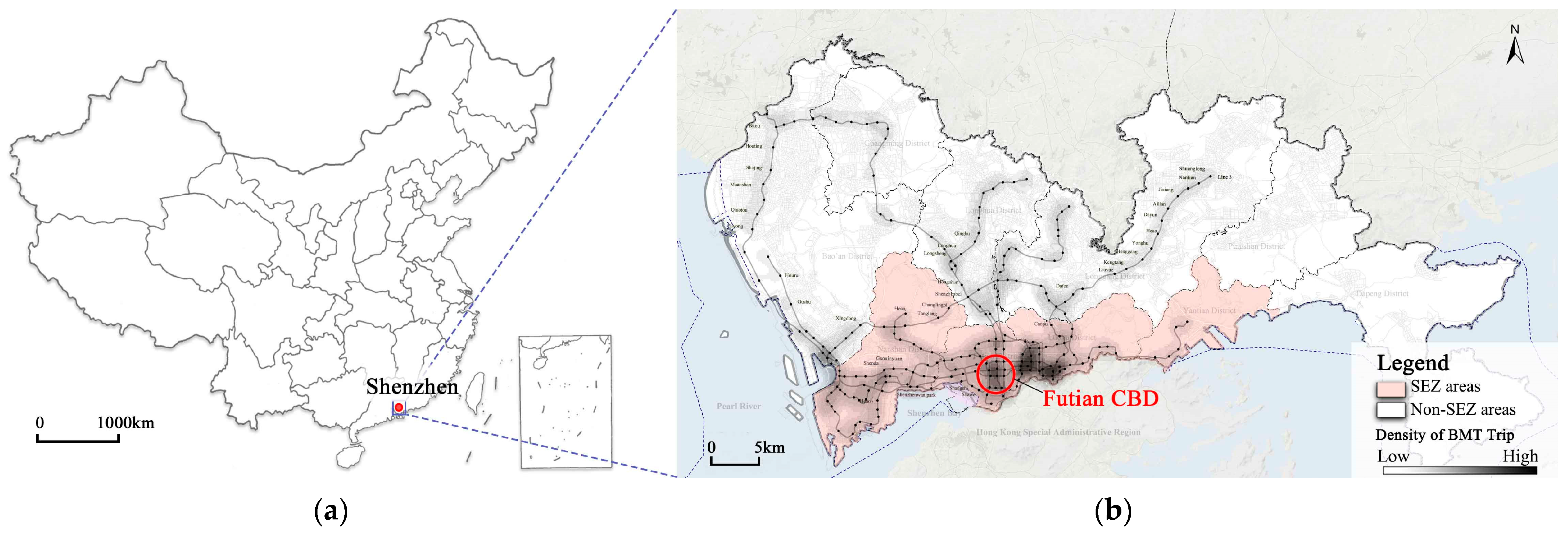
Shenzhen, located in southern Guangdong Province and adjacent to Hong Kong, is known for its high urbanization rate, rapid economic growth, and modern urban management [37]. As of February 2021, Shenzhen’s metro system comprised 10 main lines, spanning over 300 km and covering most urban areas. This extensive metro system provides an ideal foundation for studying bike–metro transfer patterns. Shenzhen’s rapid urbanization and complex socioeconomic structure make it an ideal case for exploring how the built environment influences DBS and metro transfer usage at different times and transfer flows. This study focuses on 237 metro stations operational in 2021 (Figure 1), exploring the impact of the built environment on bike–metro transfer.

Figure 1.
Study area. (a) Location of Shenzhen in China; (b) the spatial distribution of metro stations.
3.2. Data Collection
The data used in this study are as follows:
- (1)
- Metro smart card records and DBS data: Data from 1 February 2021 to 5 February 2021, covering metro smart card entries/exits and concurrent DBS ride origin–destination (OD) data (Table 1). During this period, the weather in Shenzhen was clear and the temperature was moderate.
 Table 1. Data samples (on 4 February 2021).
- (2)
- Built environment data: This dataset includes road network data, streetscape imagery, points of interest (POI) data, urban building census data, and urban land use types. Road network data cover highways, primary and secondary roads, and dedicated bike lanes. Streetscape imagery involves collecting Baidu Map street view images at 50 m intervals. The required data and their specific formats for computing the built environment are outlined in Table 2 and Table 3.
Table 2. Built environment data.
Table 3. Built environment data samples.
4. Methodology
4.1. Framework
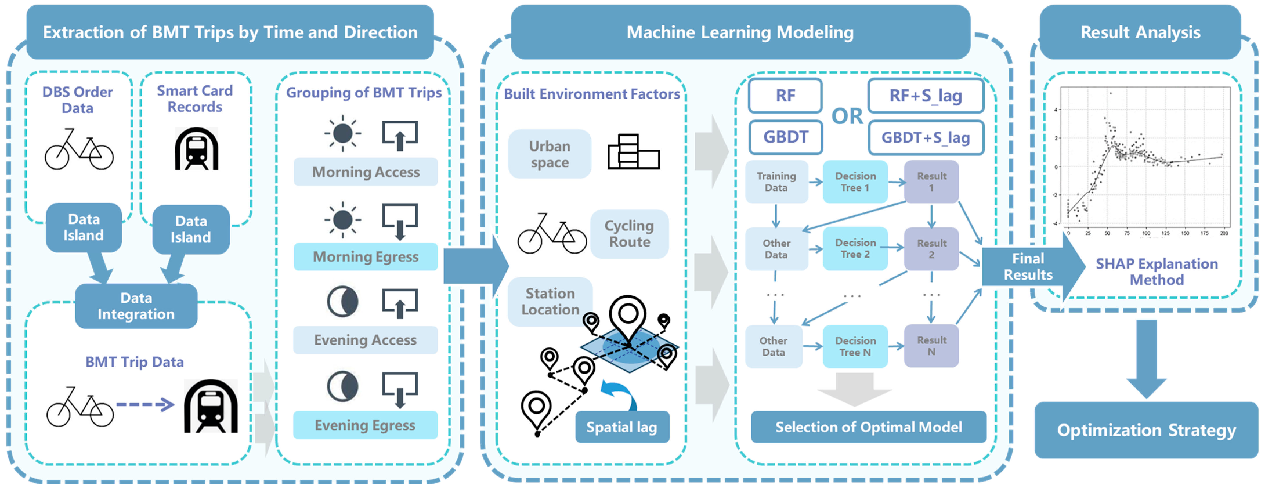
This study incorporates spatial dependence into machine learning models to analyze the nonlinear effects of the built environment on bike–metro transfer across different times and transfer directions. We introduced spatial lag variables to quantify the influence of bike–metro transfer at neighboring stations on the target station, enhancing the capture of station-to-station interactions.
To reflect spatial and temporal variations, bike–metro transfer data were categorized into four groups: morning access, morning egress, evening access, and evening egress. Each dataset includes bike–metro transfer data, built environment features, and spatial lag terms. RF and GBDT models were applied to assess the impact of spatial lag terms on model performance. SHAP analysis was used to interpret the contribution of different features to bike–metro transfer, providing a deeper understanding of the influencing factors. The overall workflow is illustrated in Figure 2.
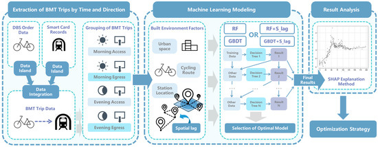
Figure 2.
Framework.
4.2. Bike–Metro Transfer Volume Calculation
We first preprocessed the cycling and metro data by removing trips with abnormal speeds, trips without changes in station entries/exits, and metro trips lasting more than 240 min. Cycling trips between 1 and 60 min were retained, while bike trips with abnormal durations were excluded [23,38].
Next, we matched the data of the DBS and metro smart card records to identify users with frequent spatiotemporal co-occurrences. The spatial constraint requires DBS trip start/end locations to be within 300 m of a metro station, and the temporal constraint ensures that the time difference between DBS and metro trips does not exceed 15 min. In total, we identified 195,503 bike–metro transfer users [11]. For this study, we focused on 384,238 trips made by 136,941 users during weekday morning and evening peak hours.
To more accurately analyze bike–metro transfer patterns, we defined the catchment area for each metro station based on cycling distances. The catchment area radius was set at the 85th percentile of cycling distances, approximately 1556 m. We used a Thiessen polygon method to divide the catchment areas, ensuring each metro station has a distinct, non-overlapping catchment area [39,40].
4.3. Spatial Dependence Analysis
We performed a spatial autocorrelation analysis to confirm spatial dependence, measuring the degree of correlation between neighboring areas. If bike–metro transfer exhibits spatial dependence, it will show significant spatial autocorrelation. We used Moran’s I to quantify this phenomenon [41], calculated as follows:
where is the total number of spatial units, and represent the observed values for units and , is the mean of the observed values, and is the spatial weight matrix, constructed based on the inverse square of the distance to describe proximity between spatial units.
4.4. Measurement of the Variables
We selected four bike–metro transfer indicators as dependent variables, representing the volume of bike–metro transfer trip entries and exits at metro stations during weekday morning and evening peak hours: morning access, morning egress, evening access, and evening egress. The independent variables covered three dimensions: trip characteristics, built environment factors, and spatial dependence. Trip characteristics included average cycling distance, transfer distance, and metro trip distance, reflecting the efficiency of the transfer system (Table 4).
Table 4.
Descriptive statistics of variables.
In terms of built environment factors, the study indicators included population density, metro station location, cycling route, and urban space. Population density variables accounted for the residential and employment populations around metro stations, reflecting regional mobility and transportation demand [42]. Station location variables included the number of stations to the city center, the number of stations to the district center, the Euclidean distance to the nearest transfer station, the coordinates of metro stations, and whether the station was located within the Shenzhen Special Economic Zone. These indicators aimed to reveal the influence of different geographical scales on bike–metro transfer.
The cycling route characteristics focus on road intersection density, bus stop density, bike lane density, slope, green view index, and sky view index. Existing research has shown that motorized transport and public transit may either compete with or complement bike usage, while the visual experience of the cycling environment, particularly green spaces and open sky views, can encourage cycling [16].
Regarding urban space, the indicators included the proportion of urban communities, urban villages, PM2.5 levels, and densities of various types of POIs, such as commercial, cultural, public, and financial. These variables reflect the spatial layout and environmental features around metro stations. POI diversity was calculated using the Shannon entropy index [43,44]. Additionally, we incorporated variables such as plot ratio, house age, and house price to capture economic conditions and development intensity in each area.
Spatial dependence plays a key role in bike–metro transfer analysis due to the interconnected nature of human mobility and urban environments [45,46], particularly in transportation trip studies [47]. Previous research has demonstrated significant spatial autocorrelation in bike–metro transfer data [11], indicating that bike–metro transfer activity at one station may be influenced by patterns at nearby stations. To account for this, we introduced spatial lag variables to quantify these interactions, enhancing our understanding of spatial relationships between stations and improving model accuracy.
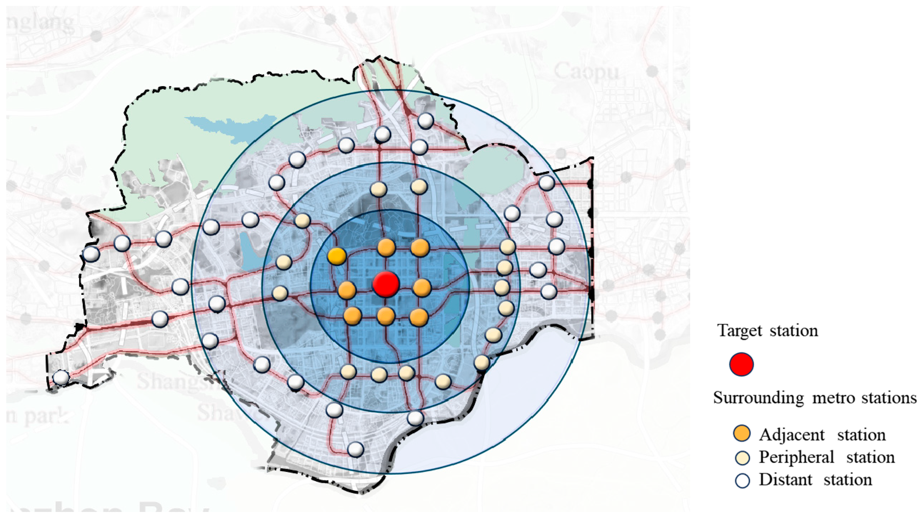
We calculated the spatial lag using an inverse distance squared weighting, assuming closer stations have a stronger mutual influence. Figure 3 shows that spatial lag was calculated as the weighted sum of bike–metro transfer at surrounding stations using the following formula:
where represents the spatial lag of station , is the Euclidean distance between stations and , and is the bike–metro transfer volume at station .

Figure 3.
Spatial lag based on inverse distance squared method.
We used the variance inflation factor (VIF) to assess multicollinearity among independent variables, ensuring that all VIF values were below 10, indicating no significant multicollinearity.
4.5. Machine Learning Models and Interpretation Methods
4.5.1. Model Construction
We applied four wide machine learning models for nonlinear prediction: RF, GBDT, XGBoost, and CatBoost [48]. These models were selected to evaluate the effect of spatial lag terms on bike–metro transfer predictions. RF and GBDT have been extensively validated in similar scenarios as robust ensemble learning methods. XGBoost and CatBoost offer improvements in optimization and performance, providing strong predictive capabilities.
To optimize model performance, we used grid search, a systematic hyperparameter tuning technique [49]. This approach involves defining candidate value ranges for each hyperparameter and iteratively testing all possible combinations. Key hyperparameters adjusted in this study included n_estimators (number of trees), max_depth (maximum tree depth), learning_rate, and subsample. The selected hyperparameters ensured the best performance on the validation set while maintaining strong generalizability.
We trained and tested models with and without spatial lag terms to assess the impact of spatial dependence on prediction accuracy. To evaluate robustness, we performed multiple random splits of the data into 80% training and 20% testing sets, repeating the training and testing processes. Results show that R2, MAE, and RMSE remain stable across data splits, confirming model reliability.
4.5.2. Model Evaluation
Model performance is assessed using three metrics: R2, mean absolute error (MAE), and root mean square error (RMSE), determined by the optimal combination of parameters. Higher R2 values and lower MAE and RMSE values indicate a better model fit. The formulas for these metrics are as follows:
where represents the actual values, represents the predicted values, and is the mean of the actual values.
4.5.3. Interpretation Methods
To interpret model predictions, we used SHAP values, which quantify each feature’s contribution to the model’s output. Positive SHAP values indicate features that enhance predictions, while negative values indicate features that diminish them. This method highlights the most influential factors and their interactions. The SHAP formula is expressed as follows:
where represents the SHAP value of feature , indicating its marginal contribution to the model’s prediction. is the size of the feature subset and is the total number of features.
5. Empirical Results
5.1. Descriptive Statistics
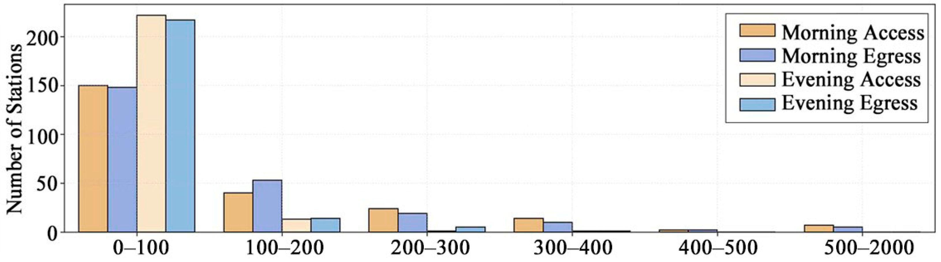
Significant differences are observed among the morning access, morning egress, evening access, and evening egress models (Figure 4). The morning access and morning egress models show significantly higher bike–metro transfer activity during the morning peak, with more dispersed trip counts than the evening access and evening egress models, which are concentrated between 0 and 50 trips. Moran’s index values for all dependent variables demonstrate notable spatial autocorrelation, confirming the presence of spatial dependence.
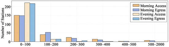
Figure 4.
Station count distribution.
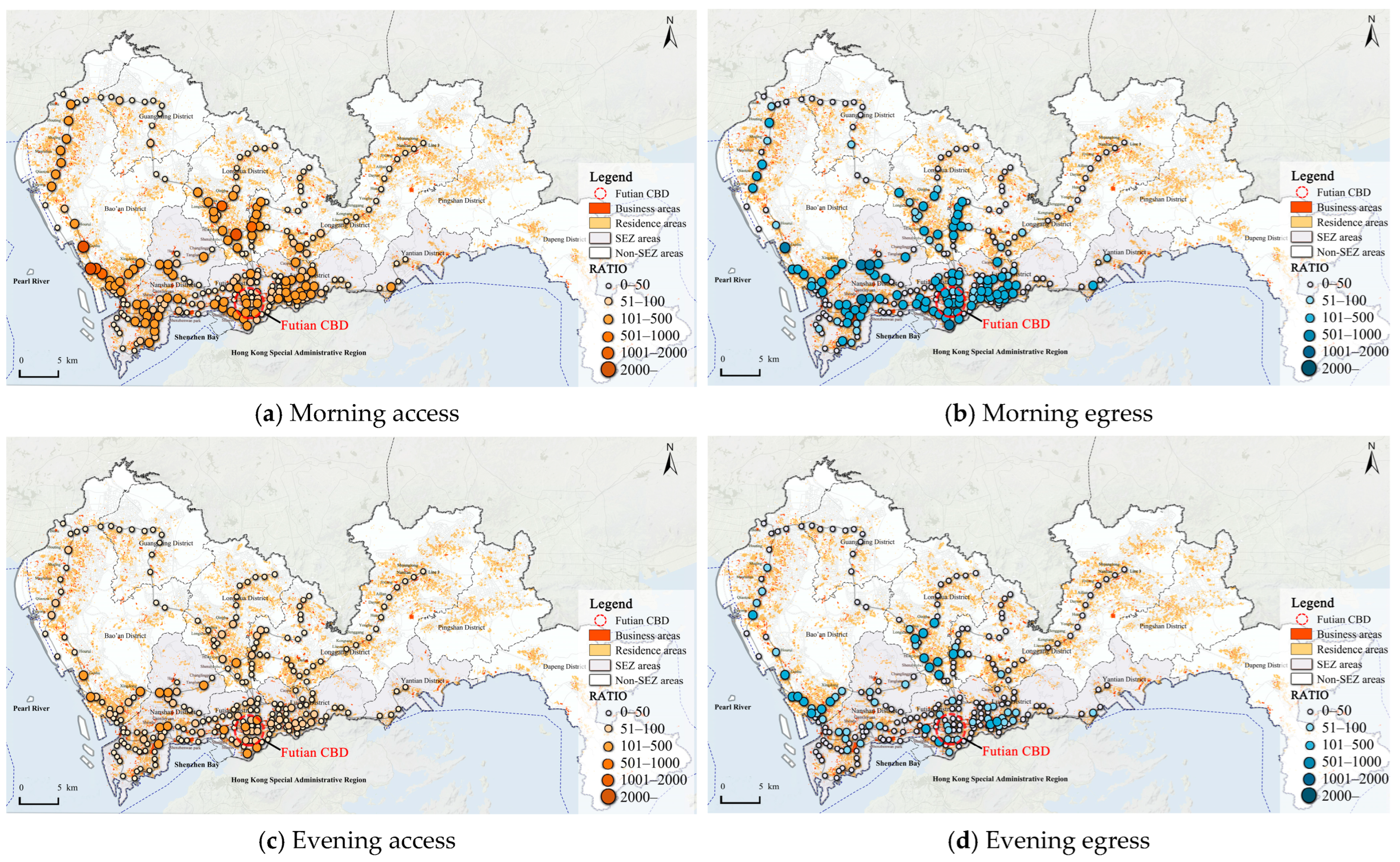
The spatial distribution reveals that morning egress and evening access are concentrated in central business districts, while morning access and evening egress are predominant in residential areas outside the Special Economic Zone (Figure 5), reflecting Shenzhen’s separation of employment and residential zones. This pattern reflects the city’s urban structure and further emphasizes the imbalance between residential and employment areas, as well as the tidal nature of trip demand.
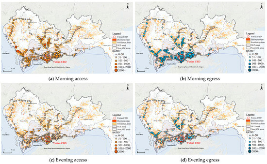
Figure 5.
The spatial distribution of bike–metro transfer.
5.2. Analysis of Overall Model Performance
This study quantifies bike–metro transfer across four variables: morning access, morning egress, evening access, and evening egress, covering peak hours in both flows. Multicollinearity tests confirmed that all independent variables have VIF values below 10, indicating no significant multicollinearity issues. Table 5 presents the optimized hyperparameter combinations and performance of both the RF, GBDT, XGBoost, and CatBoost models. After introducing the spatial lag (S-lag) variable, most models’ performance improved significantly, reflected in lower RMSE and MAE values and higher R2 values. The RF + S-lag model outperformed all others on these metrics, so it was selected for SHAP value analysis.
Table 5.
Hyperparameter optimization and performance of machine learning models.
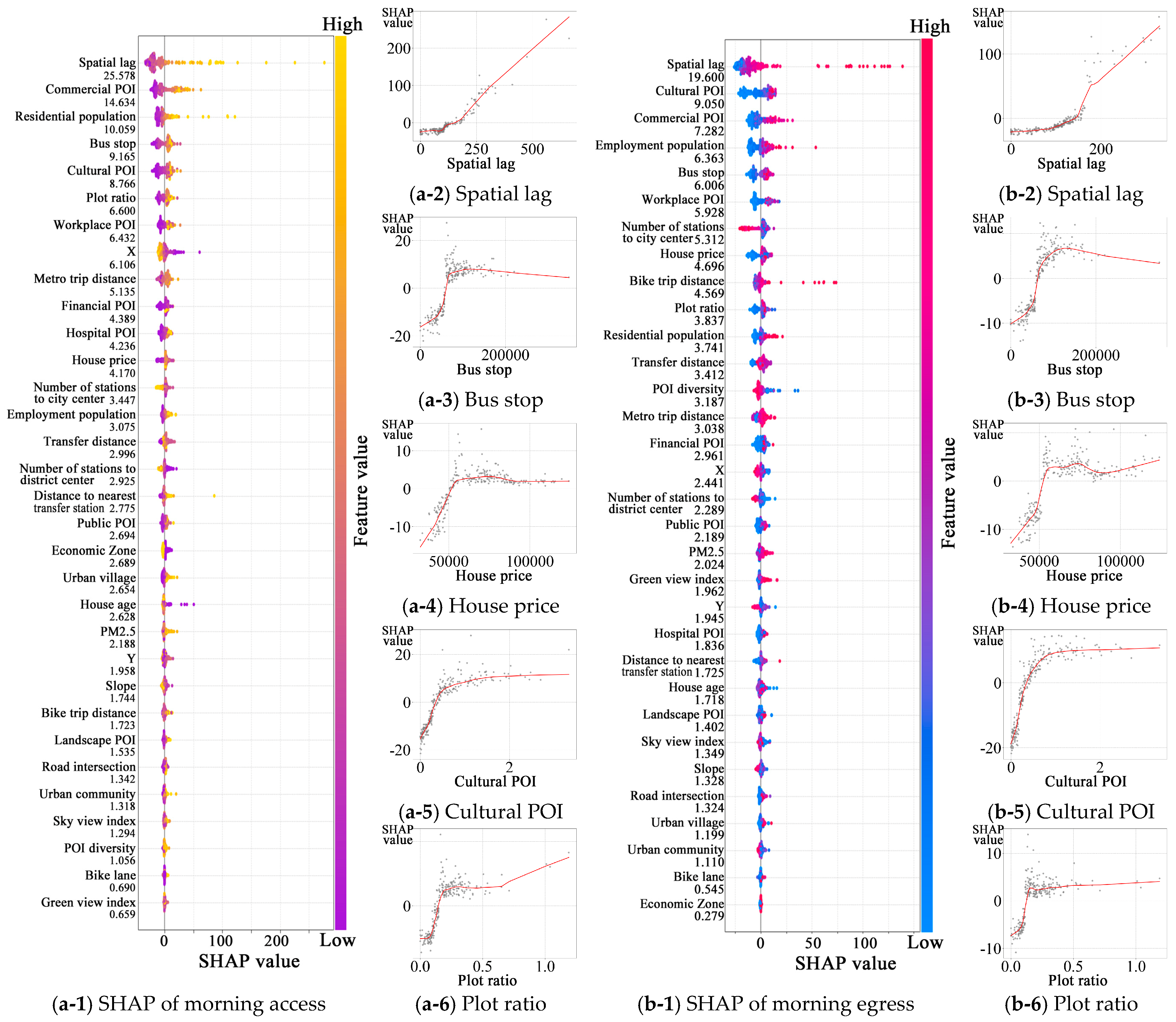
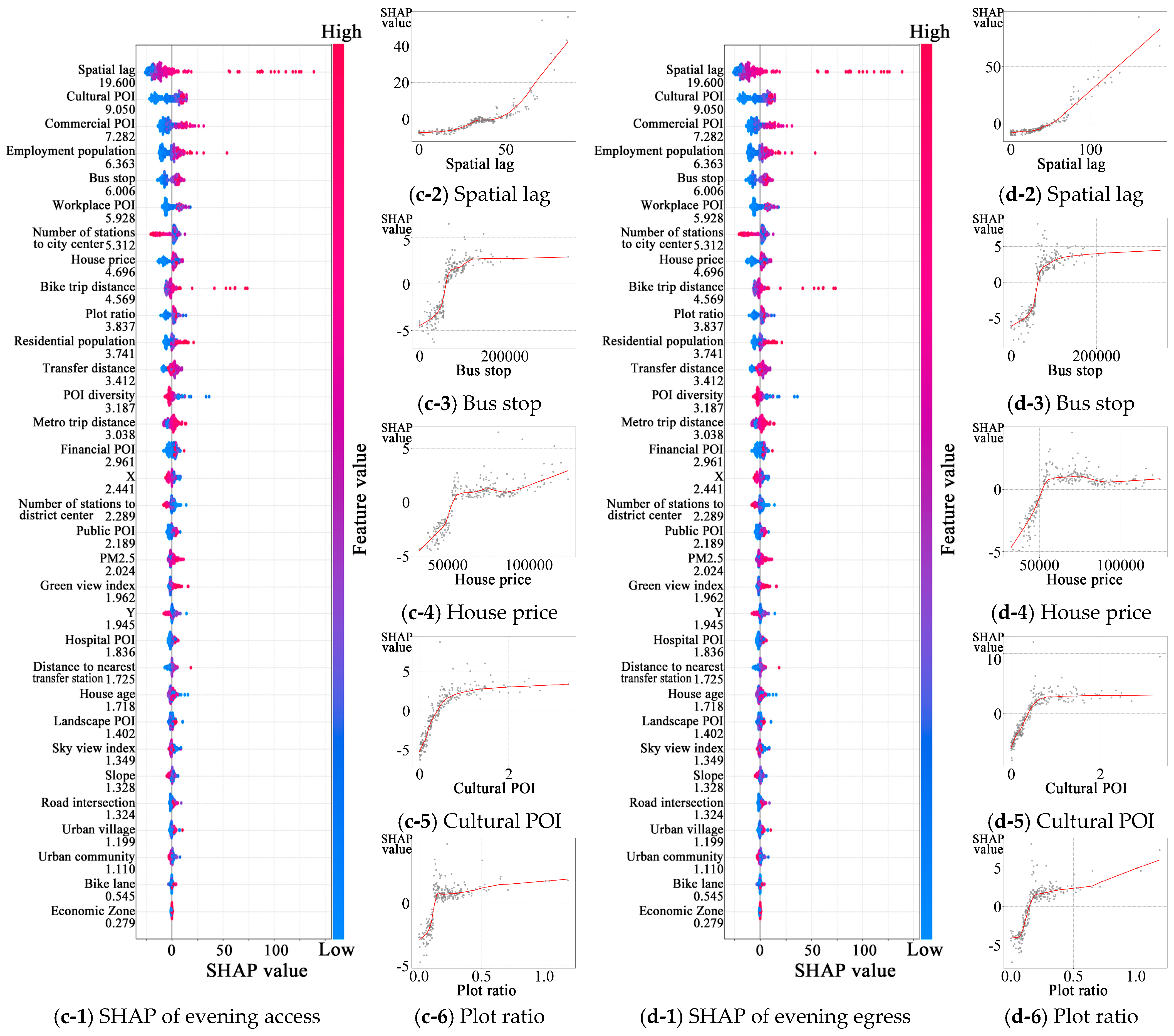
The SHAP analysis reveals the global influence of each independent variable on bike–metro transfer volume (Figure 6). In the SHAP summary plot, the y-axis lists the independent features, while the x-axis reflects each feature’s contribution to model output, with color variations indicating the magnitude of the SHAP values.

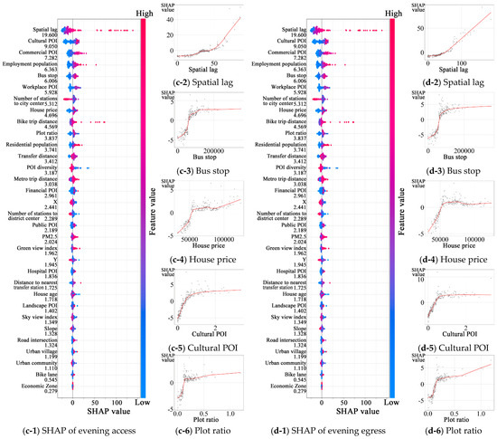
Figure 6.
SHAP summary plot for the four bike–metro transfer models.
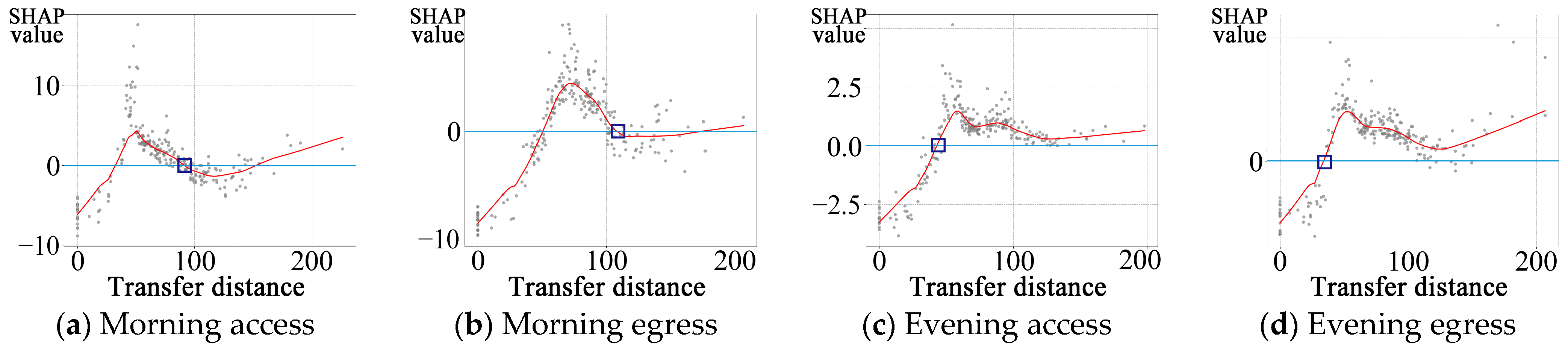
Most variables exhibit similar nonlinear effects across the four models, although the strength of their contributions varies significantly depending on the time of day and transfer flow. The spatial lag variable consistently shows the highest marginal contribution in all models. Its nonlinear effect starts negatively, then turns positive, reflecting competitive effects in low bike–metro transfer areas and reinforcing effects in high bike–metro transfer areas. Metro trip distances and transfer distances have significant impacts across all models, while bike trip distances notably influence only morning egress. Particularly, transfer distance thresholds vary by time of day: in the morning, distances of 60 to 70 m most effectively increase bike–metro transfer, while evening users are willing to trip longer distances (Figure 7).
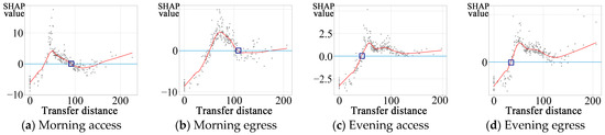
Figure 7.
Feature dependence plots of transfer distance in the four models.
Among built environment factors, station location variables have a substantial impact. The number of stations to the city center and the distance to the nearest transfer station significantly influence bike–metro transfer volume, particularly in the morning access and evening egress models. Additionally, bus stop densities above six stops/km2 contribute positively to bike–metro transfer, while bike lane density, road intersection density, and slope have lower impacts. During peak hours, cyclists tend to favor the shortest routes rather than relying on the quality of bike lanes. In terms of urban space variables, factors like plot ratio, house prices, and cultural POI density are notably impactful. Bike–metro transfer increases significantly when the plot ratio exceeds 0.2, and housing prices show a nonlinear effect, with higher bike–metro transfer in both very high- and very low-priced areas. This may occur because bicycles, as a low-cost transportation mode, are more favored in low-price housing areas, while high-price areas often provide more comprehensive non-motorized infrastructure and services [50]. The influence of cultural POI density on bike–metro transfer is particularly prominent across different times and transfer flows, possibly because areas with dense cultural POIs serve as centers of regional vitality with diverse services and attractions [51], especially under morning access and evening egress models. Commercial, work, and financial POIs are similarly influential, with commercial POIs being particularly prominent in morning access and evening egress.
SHAP analysis indicates that commercial POIs have varied effects depending on time and transfer flow, exhibiting a nonlinear effect that first reduces and then enhances bike–metro transfer. In low-density commercial areas, increasing the number of POIs may dilute demand across multiple destinations, leading to reduced bike–metro transfer. Conversely, in high-density areas, the concentration of commercial activities enhances bike–metro transfer by drawing more commuters to central hubs. This dual effect suggests that planning bike–metro transfer facilities in commercial areas must account for the potential inhibitory or stimulatory impact of commercial density. Other urban space variables, including POI diversity, healthcare POIs, green view index, and sky view index, also contribute to bike–metro transfer differently across time periods and transfer flows.
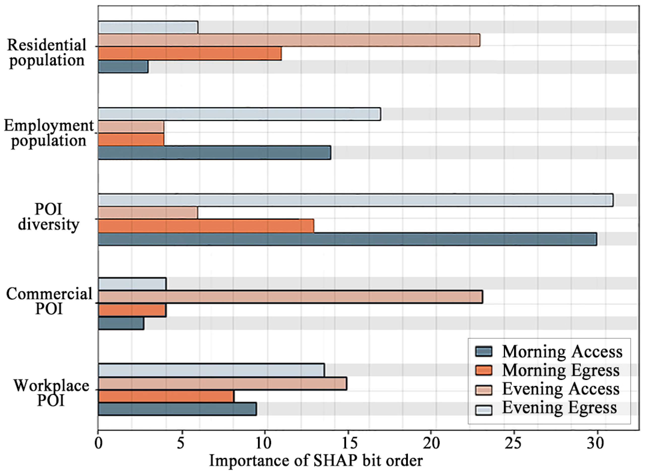
Deep analysis shows that the spatial structure of residential and employment significantly influences bike–metro transfer. Morning access and evening egress transfer are primarily driven by the residential population, while morning egress and evening access are more influenced by the employment population (Figure 8).

Figure 8.
SHAP importance ranking for residential and employment variables.
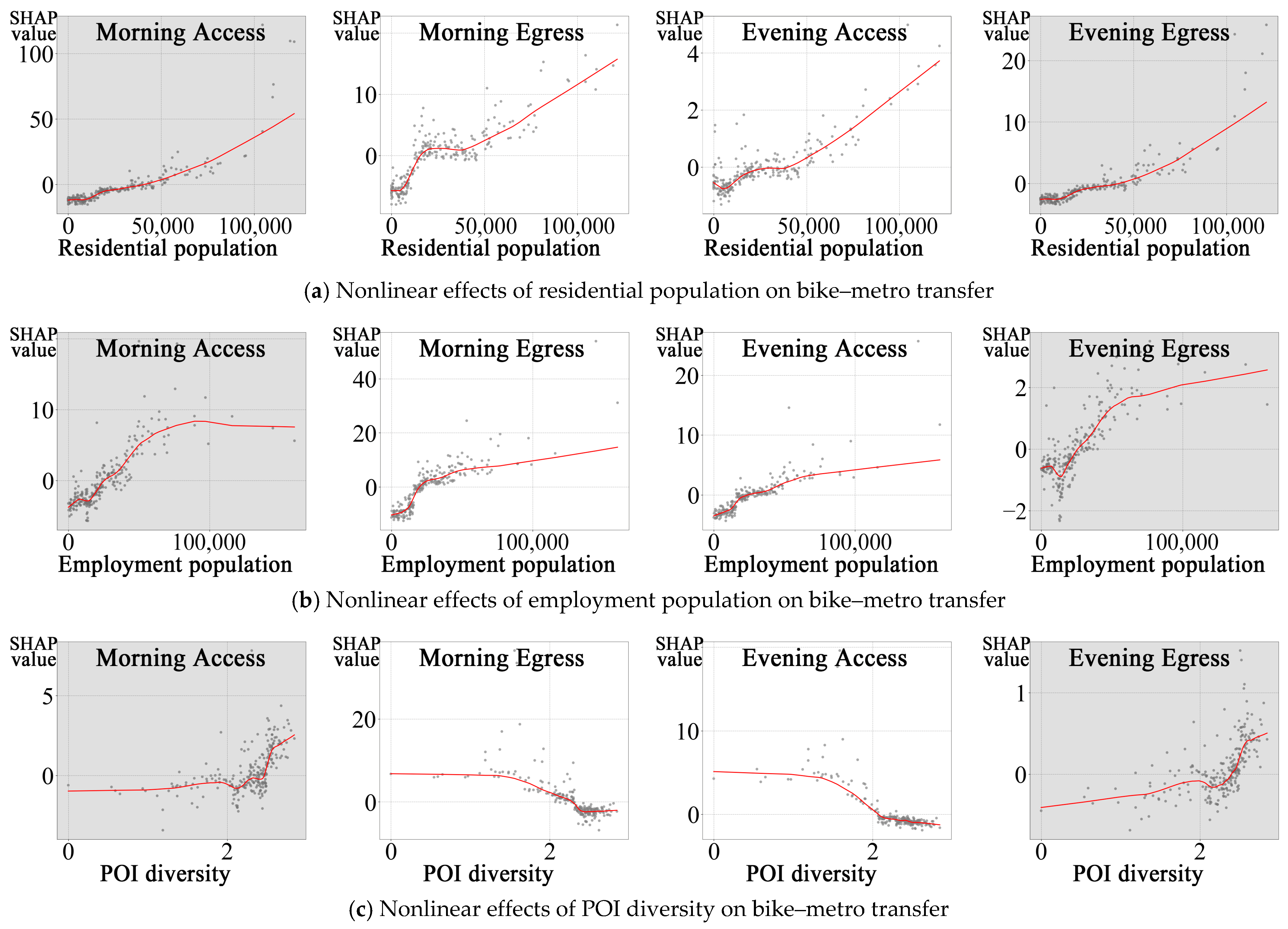
The contribution of the residential population to bike–metro transfer follows a nonlinear pattern, starting negative and turning positive, with the effect being particularly pronounced in densely populated areas, especially during morning access and evening egress models. Similarly, the employment population also exhibits a nonlinear effect, with bike–metro transfer increasing significantly when the density exceeds 20,000/km2. It is noteworthy that POI diversity shows a significant positive contribution in the evening access and morning egress models in work areas, but the opposite is observed in residential areas during morning access and evening egress models, where the contribution weakens and sometimes has an inhibitory effect after an initial boost. However, other variables closely related to the spatial structure, such as commercial and workplace POIs, do not display similar patterns (Figure 9). This trend reflects tidal traffic patterns and reveals essential differences in the factors driving bike–metro transfer across functional zones, underscoring the importance of differentiated urban planning.
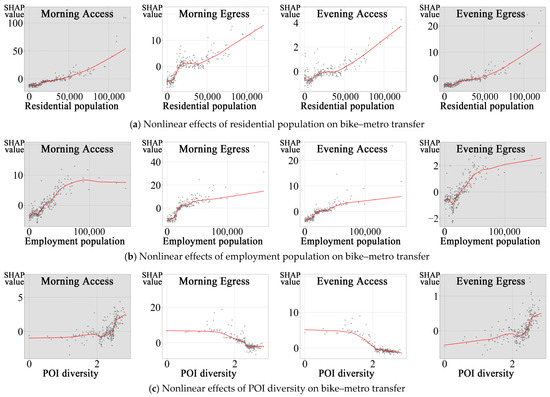
Figure 9.
Dependence plots for residential and employment variables.
5.3. Spatial Insights into Variable Contributions
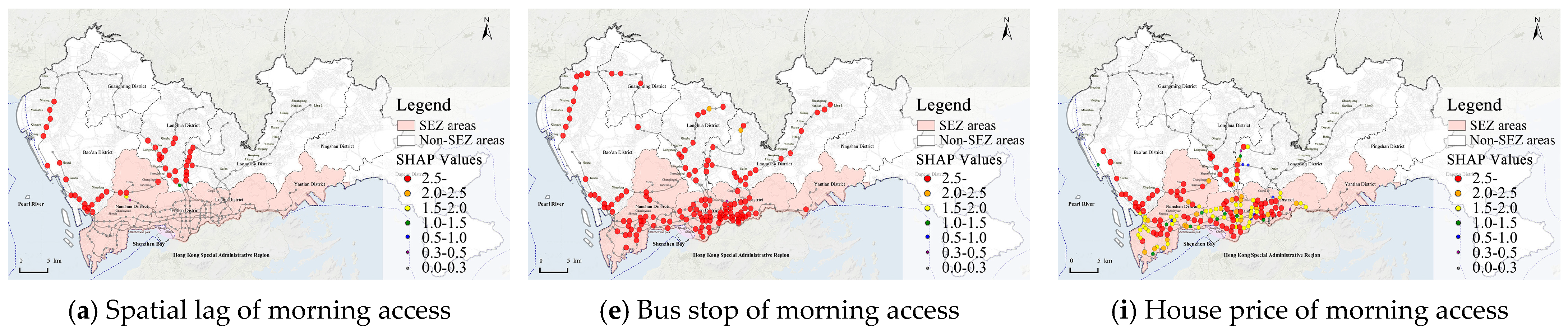
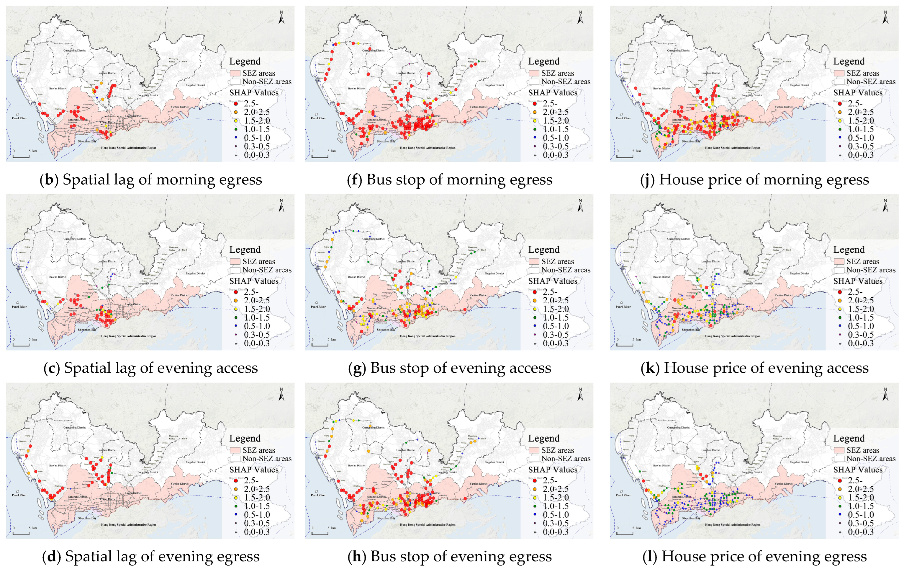
We further explored the spatial variation in the contributions of individual variables to bike–metro transfer across different regions. The contribution of the spatial lag variable is concentrated mainly in the Bao’an and Longhua districts, indicating a strong spatial dependence among stations in these areas. Bike–metro transfer at neighboring stations significantly impacts bike–metro transfer at target stations. The contribution of bus stop density is evenly distributed across districts, especially in Futian, Luohu, and Bao’an during morning peak hours. In southern Shenzhen, house prices contribute significantly to bike–metro transfer during the morning peak, likely reflecting the preference for shared bike–metro transfers among higher-income residents. Furthermore, high house prices in these areas often coincide with dense commercial and workplace POIs, further boosting bike–metro transfer (Figure 10).
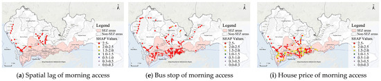
Figure 10.
Contribution of various variables to predicted BMT across different models.
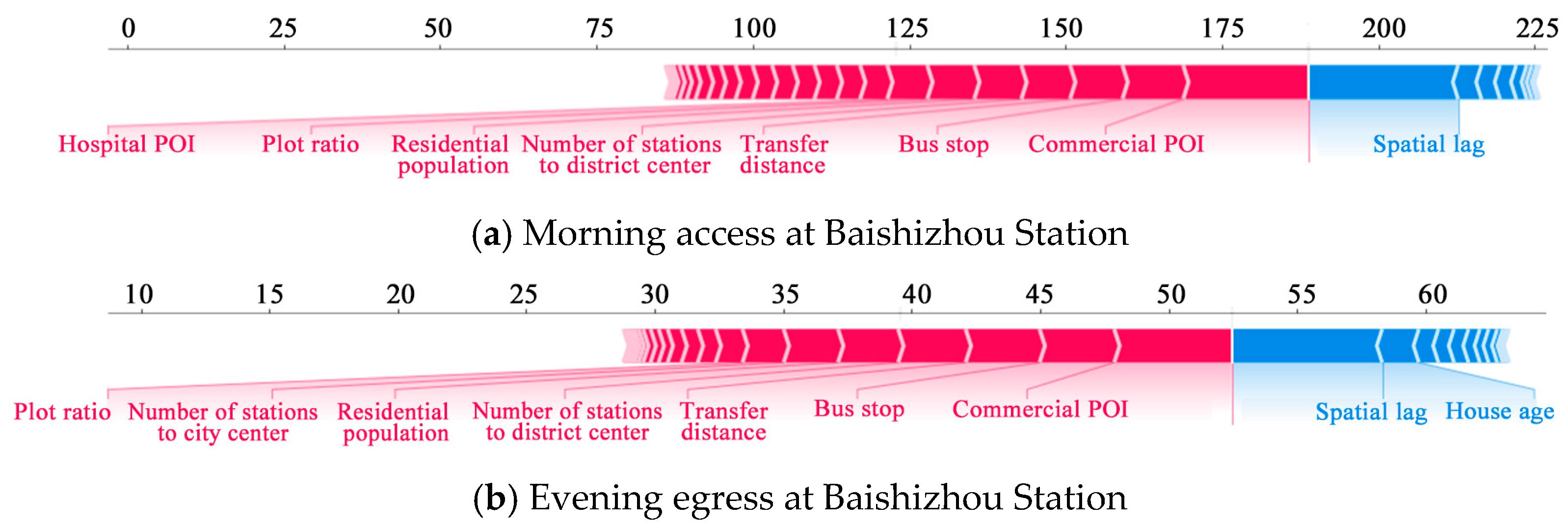
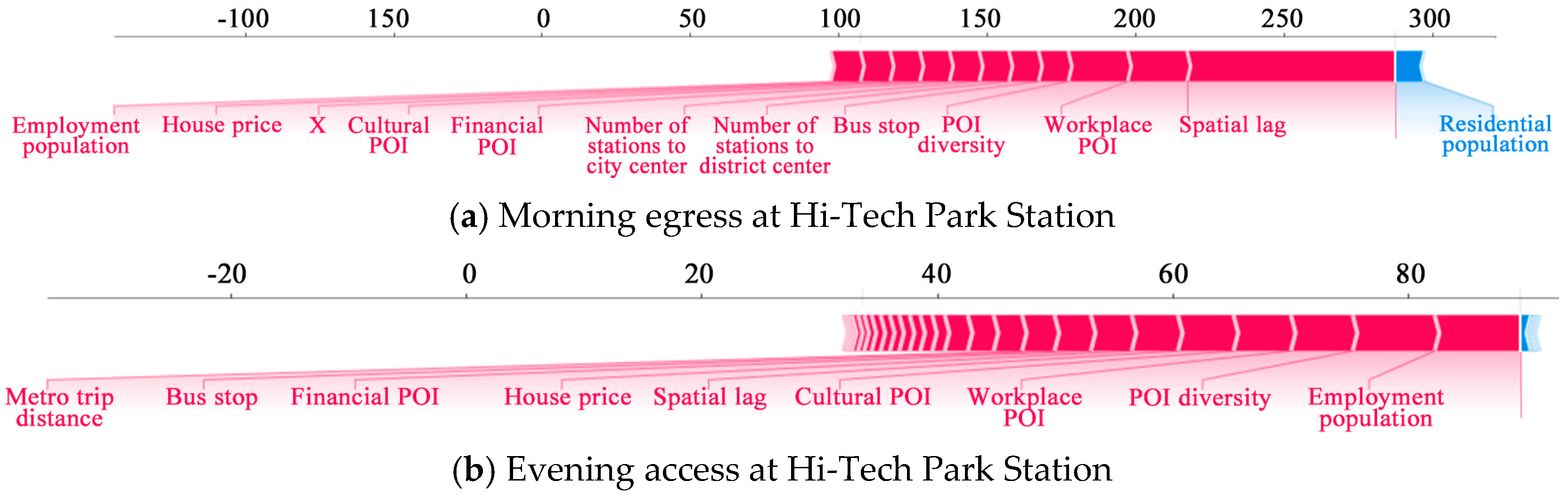
To better understand the importance of local features in the random forest model, we selected Baishizhou Station and Hi-Tech Park Station as typical cases, representing residential and employment areas, respectively. Figure 11 and Figure 12 present SHAP explanation plots for these two stations during morning access and evening egress models.
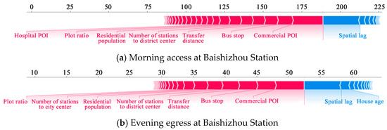
Figure 11.
SHAP explanation plot for Baishizhou Station.

Figure 12.
SHAP plots for Hi-Tech Park Station.
At Baishizhou Station, a typical urban village station, a high density of residential people surrounding the station contributed significantly to bike–metro transfer during morning access and evening egress. Commercial POIs and bus stop density were particularly influential during morning access. In the evening, the number of stations to the city center had a stronger influence on bike–metro transfer, with residents focusing on the convenience of returning home from the city center. Plot ratio and house age also played important roles during evening egress, highlighting the profound impact of a high density of residential people on bike–metro transfer. In contrast, Hi-Tech Park Station, a key technology and business hub in Shenzhen [52], exhibited different patterns. During morning egress, workplace POIs and POI diversity had the greatest contributions, reflecting the significant influence of enterprise density and diverse activities on bike–metro transfer. The spatial lag variable showed a high contribution, indicating that bike–metro transfer at neighboring stations positively influenced bike–metro transfer at this station, demonstrating an agglomeration effect. In the evening access model, the employment population and POI diversity continued to influence bike–metro transfer, while housing prices and financial POIs indicated a preference for bike–metro transfers among high-income individuals.
The analysis of local results demonstrates that bike–metro transfer at each station is influenced by multiple factors, including spatial lag effects, variations in trip timing and transfer flows, as well as built environment characteristics such as population density, POI density, land use structure, and diversity. SHAP value analysis of typical stations further illustrates how the built environment, through the spatial structure of residential and employment areas, affects transportation patterns. Providing valuable insights for optimizing bike–metro integration.
6. Discussion
6.1. Analysis of Bike–Metro Transfer Patterns
We identified 16 patterns of bike–metro transfer based on different times and transfer directions. First, we calculated the overall mean for four key variables: morning access, morning egress, evening access, and evening egress. Each variable was categorized as “High” (H) or “Low” (L) based on whether it exceeded the mean, forming 16 patterns as shown in Table 6. These patterns reflect how built environment factors influence BMT behaviors at different times and in different flows. In line with Alexander’s design pattern methodology [53,54], we consider these 16 patterns as elements of a broader “pattern language” for bike–metro integration.
Table 6.
Distribution of 16 bike–metro transfer patterns by station.
Analysis revealed that the HHHH pattern (Pattern 1) predominantly appears in core business districts and high-intensity development areas, such as Futian CBD, Qianhai, and Bantian (Figure 13). These areas exhibit high bike–metro transfer counts during both morning and evening periods, typically accompanied by overlapping high-density residential and employment zones, as well as well-developed public transportation and commercial facilities. In contrast, the LLLL pattern (Pattern 16) is found in low-density peripheral areas with low transfer counts, often at metro termini or in regions with limited development intensity, consistent with the findings of previous studies [55].
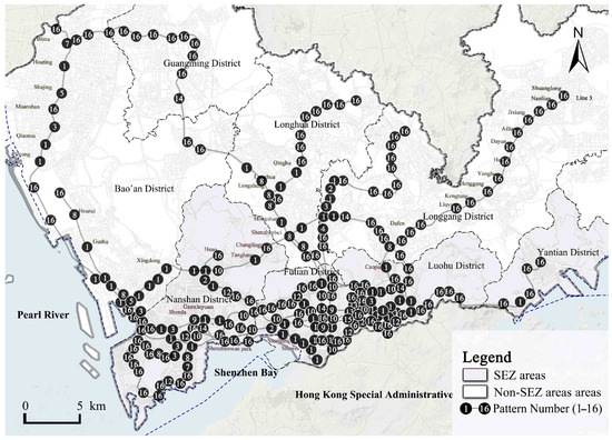
Figure 13.
Spatial distribution of bike–metro transfer patterns by station.
Excluding these extreme patterns, the other 14 patterns present multi-level, mixed characteristics. For example, patterns 2, 3, and 4 record higher values in morning access and morning egress but not necessarily in evening access or evening egress, indicating strong morning peak demand but weaker evening conditions. Patterns 5, 9, and 13 show higher values during evening hours. Patterns 6, 7, 11, 12, 14, and 15 exhibit fluctuations across different time periods, reflecting temporal influences of land use and population structure. In addition, patterns 3, 5, and 8 maintain high values in morning access and evening egress, while patterns 2, 4, 9, and 10 record higher values in morning egress and evening access, but these are not all-day phenomena. Morning access and evening egress peaks commonly occur in areas with high residential density and comprehensive living facilities, while morning egress and evening access peaks are typically associated with zones of high employment density and abundant commercial facilities. These conclusions align with previous research on cycling patterns [56,57,58].
In summary, these 16 patterns provide a systematic framework for understanding bike–metro transfer across temporal, directional, and spatial dimensions. These differences are closely associated with population, employment density, land use mix, and POI diversity, while also reflecting the resource allocation of metro and cycling integration. Inspired by the pattern language from Alexander [53] and Mehaffy [54], we propose that these patterns serve as design patterns, guiding planners in addressing diverse local conditions to create more sustainable living structures [59] and public spaces that promote well-being [60].
6.2. Applications
Based on the findings and pattern analysis, this study proposes the following planning recommendations:
First, the significant variations in bike–metro transfer patterns across times and transfer directions necessitate differentiated strategies for different areas. Flexible allocation of resources should account for the nonlinear effects of built environment factors in varying times and transfer flows. Decision-makers can use station pattern classifications to allocate resources and facilities appropriately for specific times and locations, improving public transit efficiency and accessibility. For example, at stations with an HHHH pattern, enhancing bike–metro integration facilities, such as high-standard bike lanes and parking spaces, and maintaining bus stop densities above six stops per square kilometer can improve transfer efficiency and meet the demands of high-intensity travel throughout the day. Meanwhile, deploying real-time navigation systems and big-data demand forecasts can help adjust resources effectively [54]. For stations in low-density peripheral areas with an LLLL pattern, providing basic facilities, balancing the potential inhibitory or stimulatory effects of commercial density, and activating latent demand are recommended. During morning peak hours, resources should be prioritized for stations closely connected to high-density population areas and public transit networks to improve efficiency, while areas with high transfer volumes in the evening peak should promote the development of nighttime economies to maximize the benefits of longer transfer distances.
Second, planners should address differences between residential and employment zones to match the unique factors driving bike–metro transfer in each area. For employment-dense zones, strategies to optimize morning egress and evening access include increasing bus stop density and reducing road intersection density to enhance cycling efficiency. Rational planning of plot ratios is essential to prevent overdevelopment. In residential zones, improving transfer services during peak hours by increasing commercial POI density can significantly enhance usage. Public facilities and bike network coverage can stimulate demand in low-priced housing areas while optimizing resource utilization is critical in high-priced areas. Adding cultural POIs can further attract users. Enhancing POI diversity between residential and employment zones can promote multifunctional facilities and support diverse commuting needs.
Lastly, spatial dependence must be considered in bike–metro transfer planning. The study identifies that spatial lag effects initially inhibit bike–metro transfer but later promote it. In low-transfer areas, resources should focus on enhancing core station facilities. In high-transfer areas, broader resource coverage and interactions among neighboring stations should be optimized. For example, constructing complementary bike lane networks connecting metro stations in adjacent regions can improve overall transportation system efficiency.
However, implementing these optimization strategies may face challenges such as limited resource allocation, policy coordination issues, and conflicts among stakeholders. For instance, constructing high-standard bike lanes and parking facilities requires additional financial investment and land resources, which may be constrained by existing planning frameworks, property rights, and governance systems. Stakeholder acceptance of planning adjustments may also limit implementation. Policymakers must fully consider local resource conditions and policy environments, engage in multi-stakeholder consultations, and conduct pilot studies to effectively implement planning strategies under realistic conditions [53].
7. Conclusions
This study developed a machine learning model that integrates DBS data with metro smart card records to analyze bike–metro transfer in Shenzhen across different time periods and transfer flows. The results demonstrate that accounting for spatial dependence enhances model accuracy and uncovers nonlinear effects of the built environment on bike–metro transfer across various times and transfer flows.
The study’s main contributions include (1) the development of a new bike–metro transfer analysis framework that integrates DBS order data and metro smart card records to examine bike–metro transfer trips across different peak periods and transfer flows, providing a new perspective for understanding the complex mechanisms of bike–metro transfer across various regions and time periods; (2) evaluating the impact of spatial dependence on model performance and validating the effectiveness of spatial lag variables; and (3) SHAP value analysis reveals the nonlinear influence of the built environment on bike–metro transfer at various times and in different transfer flows, providing insights for sustainable urban transportation planning.
While the analytical framework proposed in this study suggests potential applicability to dockless bike-sharing and metro integration studies in other high-density cities, this aspect warrants a more specific and detailed investigation in future research to comprehensively assess its adaptability and reliability across diverse urban contexts. Future studies should conduct comprehensive assessments in varied metropolitan settings, considering different urban structures, socioeconomic conditions, and transportation infrastructures to robustly establish the framework’s transferability.
This study, based on the case of Shenzhen, offers valuable insights that may inform sustainable transportation planning and management in similar high-density urban areas. However, this study has limitations. First, the data were collected in February 2021. Although there were no significant pandemic-related restrictions on travel activities in Shenzhen at that time, work and living patterns may have been different. Second, this study did not account for the potential impacts of varying weather and seasonal conditions on bike–metro transfer. Future research could incorporate multi-period and multi-climate analyses and validate the study’s findings in other cities. By expanding analyses across broader spatial and temporal scopes, integrating diverse environmental factors, conducting cross-city comparisons, and incorporating more comprehensive data sources, future research will enhance the understanding of bike–metro transfer patterns and provide more comprehensive references for sustainable transportation planning and management in high-density cities worldwide.
Author Contributions
Conceptualization, Y.Z. and H.L.; methodology, Y.Z. and Y.M.; software, Y.M.; validation, Y.G.; formal analysis, X.-J.C.; investigation, X.-J.C. and Y.M.; resources, H.L.; data curation, H.L. and Y.Z.; writing—original draft preparation, Y.Z., Y.M. and X.-J.C.; writing—review and editing, Y.Z., Y.M., X.-J.C. and H.L.; visualization, Y.Z., Y.M. and X.-J.C.; supervision, H.L.; project administration, Y.Z.; funding acquisition, Y.Z. and H.L. All authors have read and agreed to the published version of the manuscript.
Funding
This research was funded by the Dissertation Scholarship from the Peking University–Lincoln Institute Center for Urban Development and Land Policy (grant number DS13-20240901-ZY), and the Macau University of Science and Technology Faculty Research Grant (General Research Grants, GRF) (grant number FRG-23-002-FA).
Institutional Review Board Statement
Not applicable.
Informed Consent Statement
Not applicable.
Data Availability Statement
All data included in this study are available upon request by contact with the corresponding author.
Conflicts of Interest
The authors declare no conflicts of interest.
References
- Ibraeva, A.; de Almeida Correia, G.; Silva, C.; Antunes, A. Transit-oriented development: A review of research achievements and challenges. Transp. Res. Part A Policy Pract. 2020, 132, 110–130. [Google Scholar] [CrossRef]
- Aghaabbasi, M.; Chalermpong, S. A meta-analytic review of the association between the built environment and integrated usage of rail transport and bike-sharing. Transp. Res. Interdiscip. Perspect. 2023, 21, 100860. [Google Scholar] [CrossRef]
- van Marsbergen, A.; Ton, D.; Nijënstein, S.; Annema, J.; van Oort, N. Exploring the role of bicycle sharing programs in relation to urban transit. Case Stud. Transp. Policy 2022, 10, 529–538. [Google Scholar] [CrossRef]
- Zhou, Y.; He, Z.; Chen, J.; Ni, L.; Dong, J. Investigating travel flow differences between peak hours with spatial model with endogenous weight matrix using automatic vehicle identification data. J. Adv. Transp. 2022, 2022, 7729068. [Google Scholar] [CrossRef]
- Zhou, X.; Dong, Q.; Huang, Z.; Yin, G.; Zhou, G.; Liu, Y. The spatially varying effects of built environment characteristics on the integrated usage of dockless bike-sharing and public transport. Sustain. Cities Soc. 2023, 89, 104348. [Google Scholar] [CrossRef]
- van Mil, J.F.; Leferink, T.S.; Annema, J.A.; van Oort, N. Insights into factors affecting the combined bicycle-transit mode. Public Transp. 2021, 13, 649–673. [Google Scholar] [CrossRef]
- Morton, C.; Kelley, S.; Monsuur, F.; Hui, T. A spatial analysis of demand patterns on a bicycle sharing scheme: Evidence from London. J. Transp. Geogr. 2021, 94, 103125. [Google Scholar] [CrossRef]
- Jaber, A.; Abu Baker, L.; Csonka, B. The influence of public transportation stops on bike-sharing destination trips: Spatial analysis of Budapest City. Future Transp. 2022, 2, 688–697. [Google Scholar] [CrossRef]
- Tobler, W. A computer movie simulating urban growth in the Detroit region. Econ. Geogr. 1970, 46, 234–240. [Google Scholar] [CrossRef]
- Zhang, Y.; Thomas, T.; Brussel, M.; van Maarseveen, M. Exploring the impact of built environment factors on the use of public bikes at bike stations: Case study in Zhongshan, China. J. Transp. Geogr. 2017, 58, 59–70. [Google Scholar] [CrossRef]
- Zhang, Y.; Chen, X.-J.; Gao, S.; Gong, Y.; Liu, Y. Integrating smart card records and dockless bike-sharing data to understand the effect of the built environment on cycling as a feeder mode for metro trips. J. Transp. Geogr. 2024, 121, 103995. [Google Scholar] [CrossRef]
- Deng, Y.; He, R.; Liu, Y. Crime risk prediction incorporating geographical spatiotemporal dependency into machine learning models. Inf. Sci. 2023, 646, 119414. [Google Scholar] [CrossRef]
- Ghimire, S.; Bardaka, E. Do low-income households walk and cycle to reduce their transport costs? Insights from the 2017 US National Household Travel Survey. Int. J. Sustain. Transp. 2024, 18, 421–436. [Google Scholar] [CrossRef]
- Yin, Z.; Guo, Y.; Zhou, M.; Wang, Y.; Tang, F. Integration between Dockless Bike-Sharing and Buses: The Effect of Urban Road Network Characteristics. Land 2024, 13, 1209. [Google Scholar] [CrossRef]
- Hu, S.H.; Chen, M.Y.; Jiang, Y.; Sun, W.; Xiong, C.F. Examining factors associated with bike-and-ride (BnR) activities around metro stations in large-scale dockless bike sharing systems. J. Transp. Ge-Ography 2022, 98, 103271. [Google Scholar] [CrossRef]
- Bi, H.; Gao, H.; Li, A.; Ye, Z. Using topic modeling to unravel the nuanced effects of built environment on bicycle-metro integrated usage. Transp. Res. Part A Policy Pract. 2024, 185, 104120. [Google Scholar] [CrossRef]
- Cascajo, R.; Lopez, E.; Herrero, F.; Monzon, A. User perception of transfers in multimodal urban trips: A qualitative study. Int. J. Sustain. Transp. 2019, 13, 393–406. [Google Scholar] [CrossRef]
- Ulak, M.; Yazici, A.; Aljarrah, M. Value of convenience for taxi trips in New York City. Transp. Res. Part A Policy Pract. 2020, 142, 85–100. [Google Scholar] [CrossRef]
- Gilliland, J.; Maltby, M.; Xu, X.; Luginaah, I.; Shah, T. Influence of the natural and built environment on personal exposure to fine particulate matter (PM2.5) in cyclists using city designated bicycle routes. Urban Sci. 2018, 2, 120. [Google Scholar] [CrossRef]
- Cervero, R.; Sarmiento, O.; Jacoby, E.; Gomez, L.; Neiman, A. Influences of built environments on walking and cycling: Lessons from Bogotá. Int. J. Sustain. Transp. 2009, 3, 203–226. [Google Scholar] [CrossRef]
- Cervero, R.; Denman, S.; Jin, Y. Network design, built and natural environments, and bicycle commuting: Evidence from British cities and towns. Transp. Policy 2018, 74, 153–164. [Google Scholar] [CrossRef]
- Nielsen, T.; Skov-Petersen, H. Bikeability–Urban structures supporting cycling. Effects of local, urban and regional scale urban form factors on cycling from home and workplace locations in Denmark. J. Transp. Geogr. 2018, 69, 36–44. [Google Scholar] [CrossRef]
- Wu, X.; Lu, Y.; Gong, Y.; Kang, Y.; Yang, L.; Gou, Z. The impacts of the built environment on bicycle-metro transfer trips: A new method to delineate metro catchment area based on people’s actual cycling space. J. Transp. Geogr. 2021, 97, 103215. [Google Scholar] [CrossRef]
- Shin, H.; Cagnina, C.; Basiri, A. The impact of built environment on bike commuting: Utilising strava bike data and geographically weighted models. AGILE: GIScience Ser. 2022, 3, 15. [Google Scholar] [CrossRef]
- Mix, R.; Hurtubia, R.; Raveau, S. Optimal location of bike-sharing stations: A built environment and accessibility approach. Transp. Res. Part A Policy Pract. 2022, 160, 126–142. [Google Scholar] [CrossRef]
- Yan, Y.; Chen, Q. Spatial heterogeneity and nonlinearity study of bike-sharing to subway connections from the perspective of built environment. Sustain. Cities Soc. 2024, 114, 105766. [Google Scholar] [CrossRef]
- Bhat, C. A new spatial (social) interaction discrete choice model accommodating for unobserved effects due to endogenous network formation. Transportation 2015, 42, 879–914. [Google Scholar] [CrossRef]
- Li, Z. Extracting spatial effects from machine learning model using local interpretation method: An example of SHAP and XGBoost. Comput. Environ. Urban Syst. 2022, 96, 101845. [Google Scholar] [CrossRef]
- Schimohr, K.; Doebler, P.; Scheiner, J. Prediction of bike-sharing trip counts: Comparing parametric spatial regression models to a geographically weighted XGBoost algorithm. Geogr. Anal. 2023, 55, 651–684. [Google Scholar] [CrossRef]
- RK, P.; M. AboRas, K.; Youssef, A. Application of an ensemble CatBoost model over complex dataset for vehicle classification. PLoS ONE 2024, 19, e0304619. [Google Scholar] [CrossRef]
- Ganji, A.; Youssefi, O.; Xu, J.; Mallinen, K.; Lloyd, M.; Wang, A.; Bakhtari, A.; Weichenthal, S.; Hatzopoulou, M. Design, calibration, and testing of a mobile sensor system for air pollution and built environment data collection: The urban scanner platform. Environ. Pollut. 2023, 317, 120720. [Google Scholar] [CrossRef] [PubMed]
- Kim, S.; Lee, S. Nonlinear relationships and interaction effects of an urban environment on crime incidence: Application of urban big data and an interpretable machine learning method. Sustain. Cities Soc. 2023, 91, 104419. [Google Scholar] [CrossRef]
- Hatami, F.; Rahman, M.; Nikparvar, B.; Thill, J. Non-linear associations between the urban built environment and commuting modal split: A random forest approach and SHAP evaluation. IEEE Access 2023, 11, 12649–12662. [Google Scholar] [CrossRef]
- Kiely, T.; Bastian, N. The spatially conscious machine learning model. Stat. Anal. Data Min. ASA Data Sci. J. 2020, 13, 31–49. [Google Scholar] [CrossRef]
- Hu, S.; Xiong, C.; Chen, P.; Schonfeld, P. Examining nonlinearity in population inflow estimation using big data: An empirical comparison of explainable machine learning models. Transp. Res. Part A Policy Pract. 2023, 174, 103743. [Google Scholar] [CrossRef]
- Soltani, A.; Heydari, M.; Aghaei, F.; Pettit, C. Housing price prediction incorporating spatio-temporal dependency into machine learning algorithms. Cities 2022, 131, 103941. [Google Scholar] [CrossRef]
- Zhou, M.; Wang, D.; Guan, X. Co-evolution of the built environment and travel behaviour in Shenzhen, China. Transp. Res. Part D Transp. Environ. 2022, 107, 103291. [Google Scholar] [CrossRef]
- Wang, Z.; Yue, Y.; He, B.; Nie, K.; Tu, W.; Du, Q.; Li, Q. A Bayesian spatio-temporal model to analyzing the stability of patterns of population distribution in an urban space using mobile phone data. Int. J. Geogr. Inf. Sci. 2020, 35, 116–134. [Google Scholar] [CrossRef]
- Agnihotri, V.; Paul, S.K. Housing market shifts favouring transit-oriented development in emerging economies: The link between metro rails and housing price dynamics in Delhi. Int. J. Hous. Mark. Anal. 2024, 17, 8–31. [Google Scholar] [CrossRef]
- Gutiérrez, J.; Cardozo, O.; García-Palomares, J. Transit ridership forecasting at station level: An approach based on distance-decay weighted regression. J. Transp. Geogr. 2011, 19, 1081–1092. [Google Scholar] [CrossRef]
- Moran, P. Notes on continuous stochastic phenomena. Biometrika 1950, 37, 17–23. [Google Scholar] [CrossRef] [PubMed]
- AlQuhtani, S.; Anjomani, A. Do rail transit stations affect the population density changes around them? The case of Dallas-Fort Worth Metropolitan Area. Sustainability 2021, 13, 3355. [Google Scholar] [CrossRef]
- Kumakoshi, Y.; Koizumi, H.; Yoshimura, Y. Diversity and density of urban functions in station areas. Comput. Environ. Urban Syst. 2021, 89, 101679. [Google Scholar] [CrossRef]
- Guo, Q.; Fan, J.; Zou, K.; Qiu, B.; Zheng, Z. Influence of plant diversity and spatial pattern of urban green spaces on socioeconomic activities: Insights from Xiamen, China. Int. J. Sustain. Dev. World Ecol. 2024, 31, 330–347. [Google Scholar] [CrossRef]
- Liu, Y.; Feng, T.; Shi, Z.; He, M. Understanding the route choice behaviour of metro-bikeshare users. Transp. Res. Part A Policy Pract. 2022, 166, 460–475. [Google Scholar] [CrossRef]
- LeSage, J.; Pace, R. Introduction to spatial econometrics. In Boca Raton, 1st ed.; Chapman and Hall/CRC: London, UK, 2009. [Google Scholar] [CrossRef]
- Yang, C.; Chen, M.; Yuan, Q. The geography of freight-related accidents in the era of E-commerce: Evidence from the Los Angeles metropolitan area. J. Transp. Geogr. 2021, 92, 102989. [Google Scholar] [CrossRef]
- Ahn, J.M.; Kim, J.; Kim, K. Ensemble machine learning of gradient boosting (XGBoost, LightGBM, CatBoost) and attention-based CNN-LSTM for harmful algal blooms forecasting. Toxins 2023, 15, 608. [Google Scholar] [CrossRef]
- Belete, D.; Huchaiah, M. Grid search in hyperparameter optimization of machine learning models for prediction of HIV/AIDS test results. Int. J. Comput. Appl. 2022, 44, 875–886. [Google Scholar] [CrossRef]
- Conrow, L.; Mooney, S.; Wentz, E. The association between residential housing prices, bicycle infrastructure and ridership volumes. Urban Stud. 2021, 58, 787–808. [Google Scholar] [CrossRef]
- Kucukpehlivan, T.; Cetin, M.; Aksoy, T.; Kurkcuoglu, M.A.S.; Cabuk, S.N.; Pekkan, O.I.; Dabanli, A.; Cabuk, A. Determination of the impacts of urban-planning of the urban land area using GIS hotspot analysis. Comput. Electron. Agric. 2023, 210, 107935. [Google Scholar] [CrossRef]
- Zhang, F.; Liu, K.; Yin, L.; Zhang, F. Investigating evolutions of metro station functions in Shenzhen with long-term smart card data. In Proceedings of the Geoinformatics in Sustainable Ecosystem and Society: 7th International Conference, Guangzhou, China, 21–25 November 2019; Springer: Singapore, 2020; pp. 33–53. [Google Scholar] [CrossRef]
- Alexander, C.; Ishikawa, S.; Silverstein, M. A Pattern Language: Towns, Buildings, Construction; Oxford University Press: New York, NY, USA, 1977. [Google Scholar]
- Mehaffy, M.W.; Kryazheva, Y.; Rudd, A.; Salingaros, N.A.; Gren, A.; Mehaffy, L.; Mouzon, S.; Petrella, L.; Porta, S.; Qamar, L.; et al. A New Pattern Language for Growing Regions: Places, Networks, Processes; Sustasis Press: Portland, OR, USA; Centre for the Future of Places KTH Royal Institute of Technology: Stockholm, Sweden; UN-Habitat: New York, NY, USA, 2020. [Google Scholar]
- Gao, F.; Yang, L.; Han, C.; Tang, J.; Li, Z. A network-distance-based geographically weighted regression model to examine spatiotemporal effects of station-level built environments on metro ridership. J. Transp. Geogr. 2022, 105, 103472. [Google Scholar] [CrossRef]
- Cortina, M.; Chiabaut, N.; Leclercq, L. Fostering synergy between transit and autonomous mobility-on-demand systems: A dynamic modeling approach for the morning commute problem. Transp. Res. Part A Policy Pract. 2023, 170, 103638. [Google Scholar] [CrossRef]
- El-Assi, W.; Salah Mahmoud, M.; Nurul Habib, K. Effects of built environment and weather on bike sharing demand: A station level analysis of commercial bike sharing in Toronto. Transportation 2017, 44, 589–613. [Google Scholar] [CrossRef]
- Piatkowski, D.; Marshall, W. Not all prospective bicyclists are created equal: The role of attitudes, socio-demographics, and the built environment in bicycle commuting. Travel Behav. Soc. 2015, 2, 166–173. [Google Scholar] [CrossRef]
- Alexander, C. A Vision of a Living World. In The Nature of Order: An Essay on the Art of Building and the Nature of the Universe; Center for Environmental Structure: Berkeley, CA, USA, 2005; Volume 3. [Google Scholar]
- Mehaffy, M.W. Health and happiness in the new urban agenda: The central role of public space. Sustainability 2021, 13, 5891. [Google Scholar] [CrossRef]

Disclaimer/Publisher’s Note: The statements, opinions and data contained in all publications are solely those of the individual author(s) and contributor(s) and not of MDPI and/or the editor(s). MDPI and/or the editor(s) disclaim responsibility for any injury to people or property resulting from any ideas, methods, instructions or products referred to in the content. |
© 2025 by the authors. Licensee MDPI, Basel, Switzerland. This article is an open access article distributed under the terms and conditions of the Creative Commons Attribution (CC BY) license (https://creativecommons.org/licenses/by/4.0/).