Considering Mountain Micro-Topographic Characteristics in Habitat Quality Assessments and Its Nonlinear Influencing Mechanism

Abstract

Optimizing the habitat quality (HQ) assessment and revealing its nonlinear influence mechanisms, particularly by considering the mountain micro-topographic characteristics, are critically important for promoting sustainable development and safeguarding the ecological environment of mountain cities. Taking the Chongqing main city (CMC) as the study area, first, the Geomorphons algorithm was used to identify the mountain micro-topographic positions. On this basis, the HQ assessment of the InVEST model was optimized by collecting the multispectral data from UAV, and its spatiotemporal change trend was analyzed by the least-squares method. Secondly, hotspot analysis was used to explore the spatiotemporal differentiation of HQ on different land use and geomorphological types. Finally, based on the generalized additive model, the dominant influencing factors were determined, and their nonlinear effects were analyzed. The results showed the following: (1) The average HQ of the CMC showed an increasing trend from 2000 to 2020. The HQ of the four mountains and two rivers was higher, while it was lower in the central urban area. (2) The HQ hotspots were mainly distributed in parallel mountain areas and composed of forests, grasslands, and waters. The heterogeneity of HQ at the mountain micro-topographic scale was manifested in that the summits were always the hotspots of HQ. (3) HQ was influenced by a range of factors, including both natural environmental conditions and socio-economic drivers, among which the normalized difference vegetation index was the most important influencing factor.

1. Introduction

Biodiversity has always made an extraordinary contribution to the social economy, human survival, and well-being. Habitat quality (HQ) refers to the ability of an ecosystem to provide suitable conditions for biological survival and is an ideal indicator to reflect regional biodiversity status [1]. With the development of urbanization and industrialization, the interference of human activities on habitat has intensified, threatening regional ecological security [2]. In 2010, the 10th Conference of the Parties (COP10) of the Convention on Biological Diversity (CBD) reached the “Biodiversity Strategic Plan” (2011–2020), proposing the Aichi Biodiversity Targets [3]. In 2021, CBD COP15 further emphasized that biodiversity is the foundation of the earth’s health, human well-being, economic growth, and sustainable development [4]. China is making great efforts to promote ecological progress and is one of the first countries to incorporate biodiversity into planning decisions [5]. HQ directly influences the suitability of environments for biological species and is a critical factor in the preservation of biodiversity. The quality of different habitats directly reflects the status of regional biodiversity and ecosystem service capacity. At present, optimizing the assessment of regional HQ and clarifying its spatiotemporal evolution, hotspots differentiation, and influencing mechanism have become an important basic reference for regional biodiversity conservation and sustainable development. Therefore, strengthening HQ research holds substantial importance for safeguarding biodiversity, enhancing ecosystem service functions, and building ecological security patterns [6].

In recent years, many scholars have continuously optimized and evaluated regional HQ based on multi-source data and ecological modeling techniques to explore the influencing of different factors on HQ. The majority of studies evaluated HQ using the InVEST model [7], while others determined HQ through field surveys and by considering environmental factors such as ecosystem type and socio-economic conditions [8]. Concerning the HQ of mountainous cities, previous studies had primarily emphasized the impact of land use changes on HQ [9,10]. Some scholars also paid attention to the relationship between HQ and urban spatial morphological structure [11] and urbanization [12]. However, these studies on mountainous cities did not consider micro-topography and geomorphology characteristics to optimize the assessment of HQ. In fact, there are often differences in the habitat suitability of forestland in different parts of mountain regions, which is not considered in the current research. Most scholars concentrated on analyzing changes in HQ across various spatial and temporal dimensions [13] but ignored the spatiotemporal heterogeneity of HQ hotspots on different environmental gradients, especially on different geomorphological types. In view of the influencing mechanism of HQ, regression analysis [14], geographical weighted regression [15], and geographical detector [16] were used in most studies to analyze the linear relationships between HQ and influencing factors. In recent years, the nonlinear influence mechanism of HQ has gradually attracted researchers’ attention. Xu et al. examined the linear, nonlinear, and comprehensive impacts of different processes of habitat fragmentation on HQ by generalized additive model and geographical detector [17]. Mondal et al. used InVEST and machine learning-based ANN models to assess changes in coastal HQ in mangrove forests and analyze multiple impact factors and their nonlinear enhancement effects [18]. However, the nonlinear effects of complex landscape patterns and geomorphic combinations on HQ in mountainous cities have been neglected. Existing studies mostly focused on the effects of single factors, such as land use and landscape pattern change, on the temporal and spatial distribution of HQ [19]. However, few studies have been designed to explore the nonlinear relationship between multiple influencing factors and HQ, such as natural environment, socio-economic, and policy implementation factors. Deepening the study of spatiotemporal heterogeneity and the underlying mechanisms affecting HQ in mountain cities is beneficial for clarifying the spatiotemporal evolution of HQ and is of great significance for the sustainable development of mountain cities.

The Chongqing main city (CMC) is situated in the upper Yangtze River, within the core area of the Three Gorges Reservoir zone. It is an important ecological barrier in the upper reaches of the Yangtze River and plays an important role in the ecological security of the middle and lower reaches of the Yangtze River. As an important core city of the Chengdu–Chongqing urban agglomeration, the industrialization and urbanization of the CMC had accelerated from 2000 to 2020, with the gross regional domestic product (GDP) increasing from 58,063.45 million to 982,209 million, and the urbanization level rising from 50.26% to 93.54% [20]. With the population surging at a rate of 1.32 times, the construction land expanded by 776.93 km², and a large amount of cultivated land and forestland were occupied, with their areas decreasing by 752.64 km² and 35.43 km², respectively, which caused severe disturbance to the regional ecological environment. Therefore, it is urgent to clarify the regional HQ and its influencing mechanism to achieve a harmonious equilibrium between ecological conservation and urban growth. In view of this, CMC was selected as the research area to carry out the following work: (1) classifying geomorphological types of mountain cities and identifying the micro-topographic positions of mountains; (2) considering the micro-topography and geomorphology characteristics of mountain cities to optimize and evaluate the spatiotemporal evolution of HQ based on the InVEST model; (3) exploring the spatiotemporal heterogeneity of HQ hotspots in different geomorphological and land use types; and (4) utilizing the generalized additive model (GAM) to investigate the nonlinear relationships between various factors and HQ. The research results can provide an important reference for formulating scientific and rational biodiversity and ecological protection measures in CMC.

2. Materials and Methods

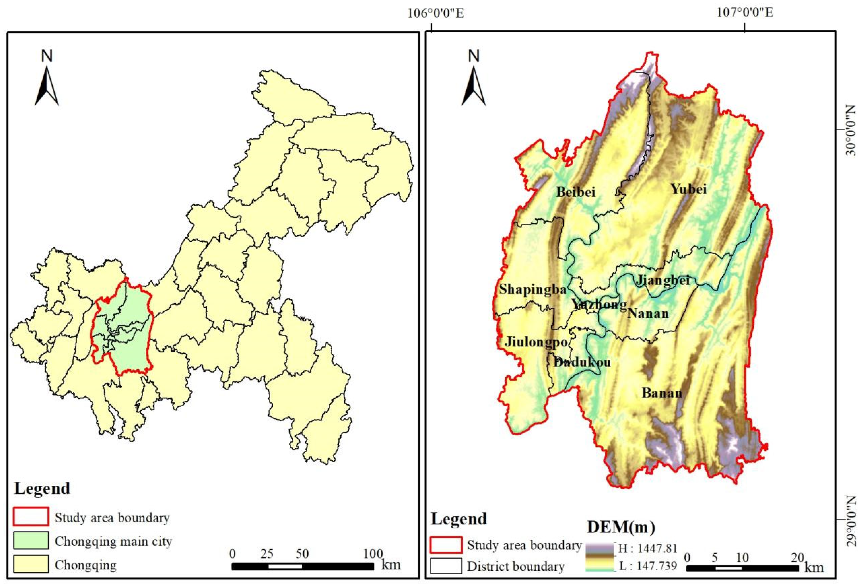
2.1. Study Area

The CMC, situated in southwestern China, serves as a transitional area between the Qinghai–Tibet Plateau and the middle–lower Yangtze River basin. It is also an important intersection and connection point of the Belt and Road strategy and the Yangtze River Economic Belt strategy [21]. The CMC (29°8′2″–30°7′37″ N, 106°14′49″–106°58′26″ E) accounted for about 6.6% of Chongqing’s total area, including 9 administrative districts: Yuzhong, Dadukou, Jiangbei, Shapingba, Jiulongpo, Nanan, Beibei, Yubei and Banan (Figure 1). The CMC is located in the parallel ridge valley area of eastern Sichuan, where the terrain conditions are complicated. Jinyun Mountain, Zhongliang Mountain, Tongluo Mountain, Mingyue Mountain, and other parallel mountains are embedded in the city from north to south, and the Yangtze River and Jialing River cut across the mountains from west to east [22], forming a basic geomorphological pattern of “two rivers and four mountains”. The overall terrain of the study area gradually decreases from the north and south sides to the middle valley zone. The terrain fluctuates greatly, and the landform types mainly include mountain, hill, platform, and flat areas. The study area is characterized by a subtropical monsoon climate featuring hot summers and mild winters. From 2000 to 2020, the urban population surged significantly, driving the rapid expansion of developed areas. This growth has directly and indirectly contributed to habitat reduction and habitat fragmentation.

2.2. Data Sources and Preprocessing

Comprehensive details regarding the data sources and processing are provided in

Table 1. Data sources and preprocessing.

Datasets	Data	Data Sources	Resolution	Data Processing
Topographic dataset	DEM, Slope, Relief, TRI, TPI, TNI, HI, VI, Cs	Geospatial Data Cloud Platform (http://www.gscloud.cn) URL (accessed on 15 September 2023)	30 m	ASTER GDEM V2 global digital elevation model (DEM) data were obtained for Slope, Relief, TRI (terrain ruggedness index), TPI (topographic position index), TNI (terrain niche index), HI (Hill index), VI (Valley index), and Cs (Surface curvature index) extractions by SimDTA V1.0.3 software.
Land use dataset	Land use types	Resource and Environment Science and Data Center (http://www.resdc.cn/) URL (accessed on 15 September 2023)	30 m	The land use type was extracted according to the scope of the study area by ArcGIS.
Meteorological dataset	Precipitation, Temperature, Sunshine duration	National Meteorological Information Center (http://data.cma.cn/) URL (accessed on 15 September 2023)	30 m	According to the daily dataset of surface climate data (V3.0), temperature, precipitation, and sunshine duration data were interpolated by ANUSPLIN 4.3 with data from 28 meteorological stations in the study area and its surrounding zones.
Vegetation dataset	NDVI, NPP	Geospatial Data Cloud Platform (http://www.gscloud.cn)URL (accessed on 20 September 2023) MODIS17 (http://files.ntsg.umt.edu) URL (accessed on 20 September 2023)	30 m, 250 m	The normalized difference vegetation index (NDVI) was calculated based on the red and near-infrared bands of Landsat remote sensing image data. The net primary productivity (NPP) obtained from MODIS17 was resampled to 30 m resolution by cubic convolution interpolation.
Soil dataset	Soil types, Sand, Silt, Clay, Gravel, Organic carbon, Bulk	National Tibetan Plateau Data Center (http://data.tpdc.ac.cn/) URL (accessed on 20 September 2023)	1 km	The soil data were extracted from the Harmonized World Soil Database v1.2 and was resampled to 30 m resolution by cubic convolution interpolation.
Distance factor dataset	Dis_forest, Dis_grass, Dis_cult, Dis_water, Dis_cons	Land use dataset	30 m	Based on the land use data of 2000, 2010, and 2020, with the ArcGIS Euclidean distance tool, the distance factor layers, such as the distance to cultivated land, forestland, grassland, water area, construction land, and unused land, were calculated.
Socio-economic dataset	GDP, POP, NLT	Resource and Environmental Science Data Center (http://www.resdc.cn/) URL (accessed on 20 September 2023) WorldPop platform (https://www.worldpop.org/) URL (accessed on 20 September 2023) NPP-VIIRS-like NLT dataset (https://eogdata.mines.edu/)URL (accessed on 20 September 2023)	1 km 500 m 500 m	The gross regional domestic product (GDP) was resampled to 30 m resolution by cubic convolution interpolation. The population (POP) was resampled to 30 m resolution by cubic convolution interpolation. The nighttime light (NLT) data were resampled to 30 m resolution by cubic convolution interpolation.

.

2.3. Methods

2.3.1. Geomorphological Types and Micro-Topographic Positions Classification

Principal component analysis (PCA), a technique for reducing data dimensionality, was utilized to identify a few comprehensive indicators containing a large amount of topographic information that were determined to replace the original topographic factor indicators. Based on the band synthesis tool, the identified principal component factors were combined into bands, and finally, the multi-band raster was unsupervised and classified using the ISODATA iterative self-organizing analysis to obtain the geomorphological types of CMC. The steps of PCA mainly include the following: (1) the deviation standardization of the original 9 topographic factors; (2) calculating the correlation and covariance matrix, eigenvalues, and eigenvectors of topographic factors (

Table 2. The percent and accumulative of eigenvalues and eigenvectors of principal components.

	Principal Component 1	Principal Component 2	Principal Component 3	Principal Component 4
Eigenvalues	12,698.092	2964.815	518.077	399.506
Percentage	73.859	17.245	3.013	2.324
Cumulative contribution	73.859	91.104	94.117	96.441
Principal component eigenvector
DEM	0.073	0.277	0.678	0.438
Slope	0.087	0.334	−0.683	0.616
Relief	0.081	0.488	−0.063	−0.440
TRI	0.078	0.427	−0.110	−0.422
TPI	0.098	−0.046	0.041	0.058
TNI	0.115	0.592	0.210	0.123
HI	0.684	−0.168	0.064	0.097
VI	−0.692	0.101	0.075	0.156
Cs	0.070	−0.023	0.054	0.069

); and (3) determining the first four principal components as the classification basis by the cumulative contribution rate.

The Geomorphons algorithm uses the topographic openness index to determine the elevation relationships between the central grid and the neighborhood grids in the other eight directions [23]. The optimal analysis window size is the key to ensuring that the terrain factors are representative in a certain range and effectively reflect the integrity of the landform. In this study, the optimal analysis window was determined to be 13 × 13 by the mean change point method [24]. Therefore, the outer search radius of the Geomorphons algorithm was set to 13, and other parameters were defaulted. Based on the r.geomorphon tool in GRASS GIS, the mountain region of CMC was divided into different micro-topographic types, namely, “summit”, “ridge”, “shoulder”, “spur”, “slope”, “hollow”, “footslope”, and “valley” [25].

2.3.2. HQ Assessment

The HQ module of the InVEST model was used to realize the assessment of HQ. The model assumes that the higher the HQ index value, the better the HQ, and the more beneficial it is for the maintenance of biodiversity. HQ depends on the relative impact and weight of each threat factor on the habitat, the habitat suitability of different land use types, and their sensitivity to threat factors. The formula is as follows:

$$Q_{xj}=H_j\times \left[1-\left(D_{xj}^z/\left(D_{xj}^z+k^z\right)\right)\right]$$

(1)

where Q_xj represents the HQ of grid x in land use type j; H_j represents the habitat suitability of land use type j; D_xj is the degree of threat faced by grid x in land use type j; k is the half-saturation constant; and z is the scaling parameter. Referring to the InVEST model user guide and related references, the default value of k is usually 0.5, and the default value of z is 2.5.

Considering the types and combinations of micro-geomorphology in the mountainous areas of the CMC, the forestlands were subdivided into five categories based on the characteristics of mountains’ micro-topographic positions, including the top-slope forestland (summit, ridge, and shoulder), the mid-slope forestland (spur, slope, and hollow), the footslope forestland, the valley forestland, and other forestlands. In this study, taking Jinyun Mountain as an example, multispectral images were collected by using DJI Phantom 4 Pro UAV in different mountains’ micro-topographic positions from 10:00 to 14:00 on 25 April 2020, when the weather was clear and cloudless. Then, the ratio vegetation index (RVI) variation coefficient was calculated to modify the habitat suitability parameters settings. It was found that the RVI variation coefficient was the highest (0.370) in the top-slope forestland, so the habitat suitability was set as 1, followed by the valley forestland (0.339) and the mid-slope forestland (0.338), and the habitat suitability was set as 0.95. The footslope forestland (0.241) was the lowest, and its habitat suitability was set to 0.9 together with other non-mountain forestlands. HQ was quantitatively evaluated using the InVEST model’s HQ module. The model integrated the land use type information, the impact intensity of threat factors, and the sensitivity of land use types to these threats in CMC (

Table 3. Threat factor maximum influence distance and weight.

Threats	Maximum Influence Distance (km)	Weight
Paddy field	1	0.5
Dry land	1	0.5
Urban land	6	1
Rural residential area	3	0.8
Industrial, mining, and transportation land	4	0.9
Bare land	1	0.6
Gross regional domestic product	3	0.3
Population	2	0.2

and

Table 4. Habitat suitability of different land use types and their sensitivity to threat factors.

Land Use Type	Habitat Suitability	Paddy Field	Dry Land	Urban Land	Rural Residential Areas	Industrial, Mining and Transportation Land	Bare Land	GDP	POP
Paddy field	0.4	0	1	0.5	0.8	0.6	0.3	0.3	0.4
Dry land	0.4	1	0	0.5	0.8	0.6	0.3	0.3	0.4
Top-slope forestland	1	0.35	0.45	0.7	0.6	0.7	0.3	0.3	0.4
Mid-slope forestland	0.95	0.45	0.55	0.8	0.7	0.8	0.35	0.4	0.5
Valley forestland	0.95	0.55	0.65	0.8	0.8	0.8	0.35	0.4	0.5
Footslope forestland	0.9	0.55	0.65	0.85	0.8	0.85	0.4	0.45	0.55
Other forestland	0.9	0.6	0.65	0.85	0.8	0.85	0.4	0.45	0.55
Grassland	0.85	0.6	0.65	0.85	0.85	0.85	0.4	0.45	0.55
Rivers	0.9	0.5	0.5	0.8	0.7	0.8	0.3	0.6	0.5
Lakes	0.9	0.5	0.5	0.7	0.8	0.8	0.3	0.5	0.5
Reservoirs and ponds	0.8	0.6	0.6	0.7	0.8	0.8	0.3	0.5	0.6
Shoal	0.8	0.5	0.5	0.6	0.6	0.5	0.4	0.2	0.2
Urban land	0	0	0	0	0	0	0	0	0
Rural residential area	0	0	0	0	0	0	0	0	0
Industrial, mining, and transportation land	0	0	0	0	0	0	0	0	0
Bare land	0	0	0	0	0	0	0	0	0

) to analyze how different habitats respond to threat factors, calculate the overall HQ index, and realize the spatial distribution pattern assessment of HQ. The HQ index, derived from analyzing the sensitivity of land use types and various threat factors within a region, serves as an indicator of regional habitat conditions. Higher index values signify superior HQ, while lower values indicate poorer conditions.

2.3.3. Least-Square Method Trend Analysis

Based on the least-squares regression model and the F-value significance test, the spatiotemporal change in HQ in CMC from 2000 to 2020 was analyzed. The linear regression equation was established with the HQ change in grid cells as the ‘a’ variable and the year as the ‘x’ variable. The slope is determined using the following formula:

$$Slope=\left(n{\displaystyle \sum _{i=1}^n{x}_i{a}_i-{\displaystyle \sum _{i=1}^n{x}_i{\displaystyle \sum _{i=1}^n{a}_i}}}\right)/\left(n{{\displaystyle \sum _{i=1}^n{x}_i^2-\left({\displaystyle \sum _{i=1}^n{x}_i}\right)}}^2\right)$$

(2)

$$\begin{array}{ll}F& =\left(ESS/1\right)/\left(RSS/\left(n-2\right)\right)\hfill \\ & =\left(n-2\right){Slope}^2{\displaystyle \sum _{i=1}^n{\left(x_i-\overline{x}\right)}^2}/\left({\displaystyle \sum _{i=1}^n{\left(a_i-\overline{a}\right)}^2}-{Slope}^2{\displaystyle \sum _{i=1}^n{\left(x_i-\overline{x}\right)}^2}\right)\hfill \end{array}$$

(3)

where slope is the change rate of the HQ; the a_i is the HQ in year x_i; and the n is the number of years. When Slope > 0, the HQ shows an increasing trend; when Slope < 0, the HQ shows a decreasing trend; when Slope = 0, the HQ shows unchanged trend. ESS is the ratio of the regression sum of squares to the explained sum of squares; RSS is the residual sum of squares. The $\overline{x}$ is the mean value of x_i. The $\overline{a}$ is the mean value of a_i. F(1, n − 2) represents the distribution with a first degree of freedom of 1 and a second degree of freedom of n − 2. When F < F_0.05(1, n − 2), it represents the HQ has no significant linear relationship with time; when F_0.05(1, n − 2) ≤ F ≤ F_0.01(1, n − 2), it represents the HQ has significant linear relationship with time; when F ≥ F_0.01(1, n − 2), it means the HQ has dramatic significant linear relationship with time. According to the critical value table of F_α distribution, it shows F_0.05(1, 1) = 161.448 and F_0.01(1, 1) = 4052.181. Based on the slope of linear regression and F-value significance test results, the seven categories of HQ temporal change trend were obtained by reclassification and spatial superposition (

Table 5. The categories of HQ temporal change trend.

Slope	F-Value	Change Trend Types
Slope = 0	F < 161.448	unchanged
	161.448 ≤ F < 4052.181
	F ≥ 4052.181
Slope > 0	F < 161.448	nonsignificant increase
	161.448 ≤ F < 4052.181	significant increase
	F ≥ 4052.181	dramatic increase
Slope < 0	F < 161.448	nonsignificant decrease
	161.448 ≤ F < 4052.181	significant decrease
	F ≥ 4052.181	dramatic decrease

).

2.3.4. Hotspot Analysis

Hotspot analysis of HQ can describe the spatial clustering and dispersion of HQ. Areas with high values are identified as hotspots, while areas with low values are identified as coldspots. In this study, the Getis–Ord G_i^* index in ArcGIS was used to identify spatial clusters of HQ. The specific formula is as follows:

$$G_i^{*}={\displaystyle \frac{{\displaystyle {\sum }_{j=1}^n{w}_{i,j}{x}_j-\overline{x}{\displaystyle {\sum }_{j=1}^n{w}_{i,j}}}}{S\sqrt{\frac{\left[\mathrm{n}{\displaystyle {\sum }_{j=1}^n{w}_{i,j}^2-{({\displaystyle {\sum }_{j=1}^n{w}_{i,j}})}^2}\right]}{n-1}}}}$$

(4)

$$\overline{x}={\displaystyle \frac{{\displaystyle {\sum }_{j=1}^n{x}_j}}{n}}$$

(5)

$$S=\sqrt{{\displaystyle \frac{{\displaystyle {\sum }_{j=1}^n{x}_j^2}}{n}}-{\left(\overline{x}\right)}^2}$$

(6)

where x_j represents the attribute value of feature j, w_i,j denotes the spatial weight between feature i and j, and n is the total number of features. When the calculated result G_i* > 0, it indicates a high-value aggregation distribution in the corresponding area, which represents a “hotspot” of HQ index; when G_i* < 0, it shows a low-value aggregation distribution in the corresponding area, representing a “coldspot” of HQ index [26]. According to the analysis results, the study area was divided into five categories: hotspots and coldspots (99% confidence), sub-hotspots and sub-coldspots (90% confidence), and nonsignificant areas.

2.3.5. Distribution Index

The spatial heterogeneity of HQ hotspots in different landforms can be visually observed by using the distribution index. The formula is as follows:

$$P=\left(S_{ie}/S_i\right)/\left(S_e/S\right)$$

(7)

where P is the distribution index; S_ie represents the area of the i-th HQ hotspots on the e-th landform; S_i represents the total areas of the i-th HQ hotspots; S_e represents the total areas of the e-th landform; and S represents the total areas of the entire study area. When p > 1, it indicates that the HQ hotspots have a high distribution frequency on a certain landform and are dominantly distributed. The larger the p-value, the higher the degree of distribution dominance.

In order to better reveal the relationship between mountain micro-geomorphology and the distribution of HQ hotspots, focusing on mountain regions, the distribution difference of hotspots in different micro-geomorphology types was further analyzed. In the above formula, S_ie represents the area of the i-th HQ hotspots on the e-th micro-geomorphology, and S_e represents the total area of the e-th micro-geomorphology. S represents the total area of all mountains.

2.3.6. Generalized Additive Model

The GAM was employed to detect nonlinear regression effects of influencing factors. The model formula is as follows:

$$g(\mu )={\beta }_0+x_i\beta +{\displaystyle \sum _{j=1}^n{f}_j(x_{ij})}+\epsilon$$

(8)

where g represents the link function; µ denotes the expected value of dependent variable Y; β₀ is the intercept term; x_i and β are the independent variables and fixed-effects parameters, respectively; f_j(x_ij) refers to non-parametric smoothing functions; and ε is the error term.

In this study, the CMC was divided into 5468 grids of 1 km × 1 km, and the grid center points were extracted as sample points. The HQ and influencing factors were extracted to the sample points as dependent variables and independent variables, respectively, and the data of three years were merged into a data set with a sample size of 16,404. Initially, 33 influencing factors were selected based on data availability and rationality, taking into account the natural environment, socio-economics, and policy implementation (

Table 6. The VIF of influencing factors.

Influencing Factors	VIF	Influencing Factors	VIF	Influencing Factors	VIF
Land use types	2.05	Temperature	>5	Distance to cultivated land	2.05
Landform type	1.27	Precipitation	1.71	Distance to construction land	1.77
DEM	2.35	Rainfall erosivity index	>5	POP	1.60
Slope	1.74	Reference evapotranspiration	>5	GDP	3.54
Aspect	1.05	Soil types	>5	Nighttime light	>5
Relief	>5	Erodibility	>5	CMC overall urban planning	>5
TRI	>5	Saturated hydraulic conductivity	>5	Multi-center groups strategies	1.84
TPI	1.04	Organic carbon content	1.35	Four parallel mountain developments and controls	2.01
TNI	3.24	Distance to forestland	1.56	Ecological function regionalization	>5
NDVI	2.99	Distance to grassland	1.14	Ecological redline	2.68
NPP	3.62	Distance to waters	1.23	Beautiful landscape city planning	2.35

). To avoid overfitting the model, the collinearity test was performed based on the variance inflation factor (VIF). Ultimately, 22 influencing factors with a VIF below 5 were selected to build GAM [27]. The adjusted determination coefficient R² of the model reached 0.871, indicating that the model had excellent performance and goodness of fit [28]. The significance of categorical and numerical variables was tested by t-value and F-value, respectively, where *** p < 0.001 means extremely significant; ** p < 0.01 means very significant; and * p < 0.05 means significant. And, the GAM analysis was conducted using R 3.6.1 with the mgcv package.

3. Results

3.1. Topographic Features of Mountain City

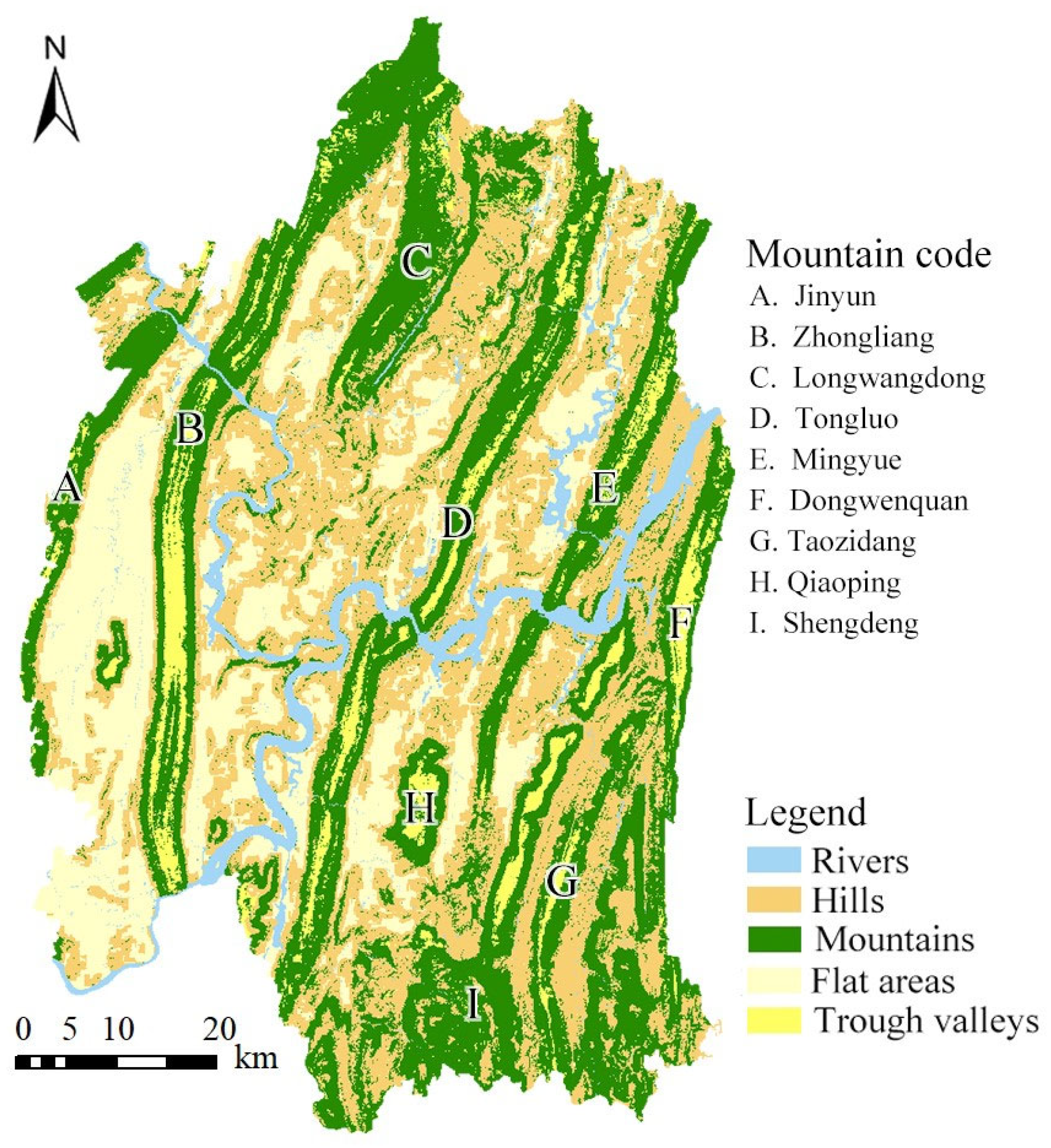
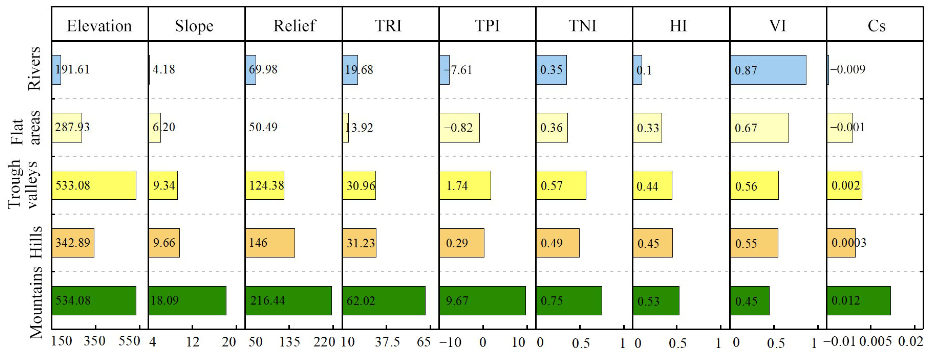
3.1.1. Landform Type Characteristics of CMC

The overall terrain of the CMC was higher in the northeast and southeast and gradually decreased to the central valley, with an average elevation of 392.58 m. There were five landform types in CMC, namely flat area, trough valley, mountain, river, and hill (Figure 2). Mountains and hills were the main landform types, with an area proportion of 34.29% and 34.60%, respectively. There were many parallel anticline mountains, such as Jinyun Mountain, Zhongliang Mountain, Tongluo Mountain, and Mingyue Mountain, which were wedged into the CMC from northeast to southwest. Except for the VI, all topographic indexes in the mountains had the highest value; the average elevation and slope were 534.08 m and 18.09°, respectively, and the relief reached 216.44 (Figure 3). Hills were mainly distributed on both sides of mountains, southeast and northeast of CMC, with the average elevation and slope of 342.89 m and 9.66°, respectively. The relief and TRI of hills were second only to the mountains. The trough valleys were distributed at the top of the anticline mountains, with an area proportion of 5.96%. The average elevation of the trough valleys was 533.08 m, second only to mountains, and the relief was slightly lower than that of hills. Flat regions comprised 20.12% of the total area and were predominantly located in the syncline valley area, alternating with hills. Notably, the largest expanse of flat terrain was found between Jinyun Mountain and Zhongliang Mountain. The average elevation and slope of the flat areas were only 287.93 m and 6.20°. The TPI and Cs were close to 0. The rivers had the lowest average elevation, with a TPI of −7.61 and a VI as high as 0.87, indicating that the rivers were primarily located in valley regions.

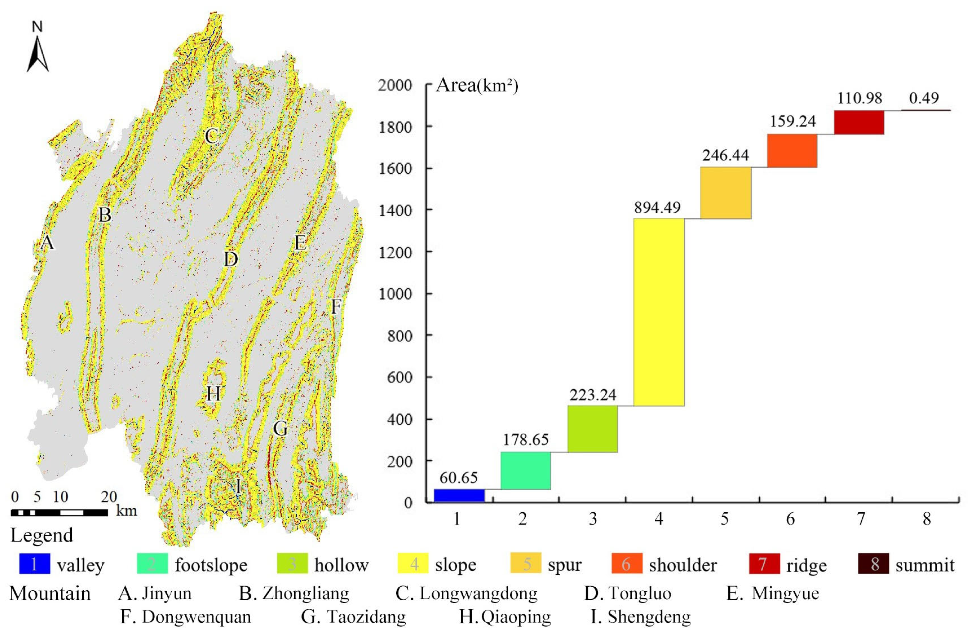
3.1.2. Mountain Micro-Topographic Analysis of CMC

To further examine the HQ heterogeneity across different micro-geomorphology types in the mountain region, this study selected the mountains from the above topographic division results to classify micro-geomorphic types and extract the information of mountain micro-topographic positions. Based on the Geomorphons method, the micro-geomorphology types and their combinations in the mountains were divided into eight different mountains’ micro-topographic positions (Figure 4), namely summit, ridge, shoulder, spur, slope, hollow, footslope, and valley.

The summits, ridges, and shoulders together constituted the skeleton of mountain terrain, and all belonged to the top region of the mountains. The area of summits was 0.49 km², accounting for only 0.03% of the mountains. In addition to the VI, the values of all topographic indices were higher, and the average elevation and slope were the highest, reaching 674.28 m and 20.46° (Figure 5). The ridges areas accounted for 5.92%, mainly extending along the middle of parallel mountains and the edge of trough valleys. The TPI, HI, and Cs of the ridges were second only to summits, and the average elevation was 531.31 m. The area proportion of the shoulders was 8.50%, and its average elevation was second only to summits, and the relief and TPI were low, which was relatively flat.

The spurs, slopes, and hollows were distributed alternately, and all belonged to the middle of the mountains, forming the main body of the mountain. The area proportions of these three micro-geomorphology types were relatively high, among which the slopes account for as high as 47.73%. Because they were located in the middle of the mountains, the slope, relief, TRI, and TPI were high, and the average elevation, TPI, HI, and Cs were the highest on spurs and the lowest on hollows.

The footslopes and valleys had the lowest elevation, accounting for 9.53% and 3.24% of the CMC, respectively, which belonged to the bottom region of the mountains. The difference was that the footslopes gradually transited to the flat, with the lowest slope and gentle terrain. The valley was a linear, extended trough-shaped depression formed by scouring, mostly located on the watershed line, with the highest VI and a certain degree of undulation and complexity.

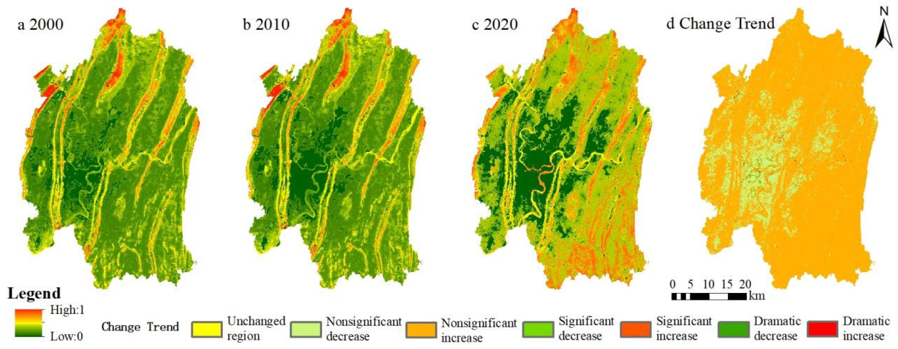
3.2. Spatiotemporal Change Trend Characteristic of HQ

On the overall spatial scale, Jinyun Mountain, Zhongliang Mountain, Tongluo Mountain, Mingyue Mountain, and other elevated regions exhibited higher HQ compared to the central urban zones. And the growth trend of HQ in southeastern mountainous areas was particularly significant in 2020 (Figure 6). On a time scale, the average HQ showed an improving trend from 2000 to 2020, which was 0.151, 0.152, and 0.373, respectively, especially in the period from 2010 to 2020. From 2000 to 2020, there were significant regional differences in the HQ change trend in CMC (Figure 6d), and the changing trend of the urban central areas generally showed a nonsignificant decreasing trend. Also, there were significant and dramatic significant decreases in areas, and the total area showing a decreasing trend was 810.64 km², of which 97.20% belonged to the area with a nonsignificant decrease in HQ, which was mainly closely related to the overall urban planning and expansion direction. As a whole, the four mountains and the southeastern areas showed a nonsignificant increasing trend, and there were also significant and dramatic significant increases in areas. The total area showing an increasing trend was 4651.83 km², accounting for 85.16% of the whole study area. Among these, the majority of the region showed a nonsignificant increase, representing 99.64% of the total area. The smallest portion, covering only 0.0324 km², remained unchanged in HQ.

From the perspective of administrative districts, Beibei, Banan, and Yubei had higher levels of HQ, with average HQ indices of 0.266, 0.257, and 0.224. While Yuzhong was the lowest, with an average HQ index of only 0.094 (Figure 7). The average HQ in Beibei and Banan increased from 2000 to 2020, and other administrative districts showed an overall trend of slightly decreasing first and then increasing. And the HQ increased the most from 2010 to 2020. Banan had the largest change in average HQ, rising by 0.330, followed by Beibei and Yubei, with changes of 0.199 and 0.196, respectively. The change in average HQ in Jiangbei was the smallest, with an increase of only 0.09, followed by Dadukou, with a smaller change of 0.106. By 2020, the HQ index in Banan was the highest (0.476), and the lowest was 0.200 in Yuzhong.

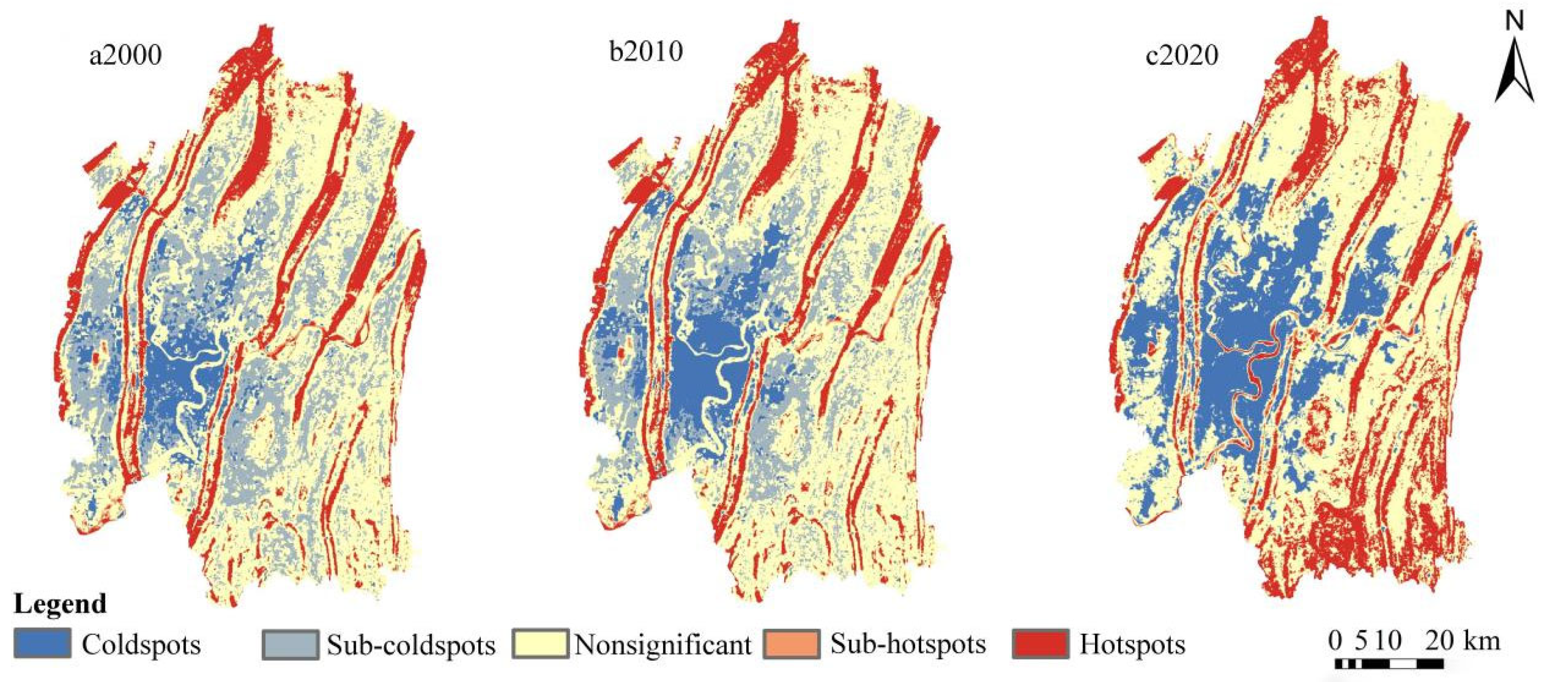
3.3. Spatiotemporal Heterogeneity Analysis of HQ Hotspots

The hotspot identification of HQ for the CMC revealed distinct spatial differences, with notable differentiation between coldspots and hotspots (Figure 8). The hotspots were predominantly located in the mountain areas encompassing Jinyun Mountain, Zhongliang Mountain, Tongluo Mountain, and Mingyue Mountain, and the whole area was in a band from northeast to southwest. The sub-hotspots were mostly distributed at the edge of hotspots and were less distributed. The coldspots of the HQ index were mainly distributed in the central and western sections of the study area, corresponding to the urban central areas of CMC, where the low value of the HQ index was clustered due to rapid urban development and frequent human activities. The sub-coldspots were distributed on the edge of the coldspots. The flat areas on the north and south sides of the study area had no significant features.

On a time scale, the area of HQ hotspots in 2000, 2010, and 2020 were 838.14 km², 837.62 km², and 1086.16 km², indicating an upward trend. From 2000 to 2010, the spatial distribution and area of hotspots were almost unchanged. Between 2010 and 2020, the total area of hotspots increased by nearly 30%, especially in the southeastern mountainous areas. Over the past two decades, the rapid urbanization and spread of built-up areas have led to a significant growth in the total area of HQ coldspots within the study area, expanding from 412.58 km² in 2000 to 1042.60 km² in 2020, with an increase rate of nearly 150%. The newly added coldspots were predominantly concentrated around the edges of existing coldspots, aligning closely with the pattern of urban sprawl. The original large area of sub-coldspots and nonsignificant areas were transformed into coldspots, which caused the total area of sub-coldspots to shrink seriously, from 1287.55 km² to 287.79 km².

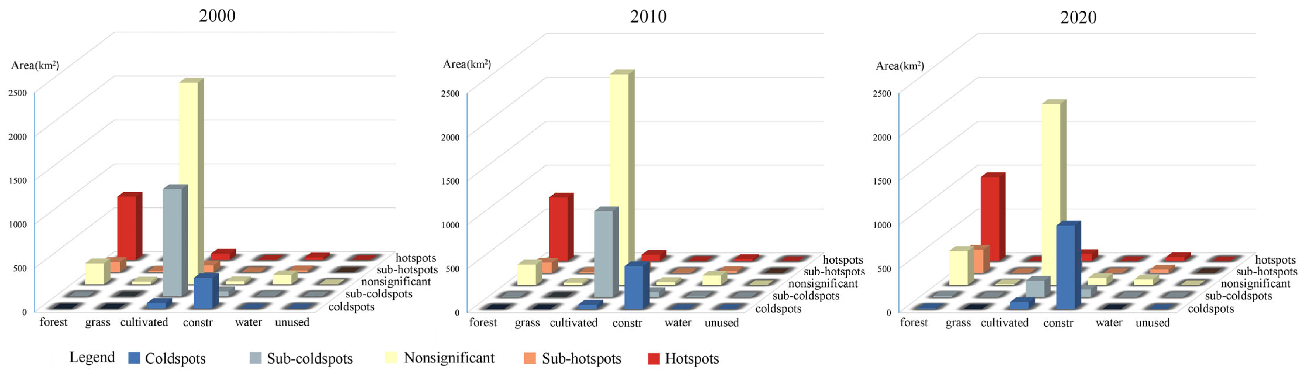
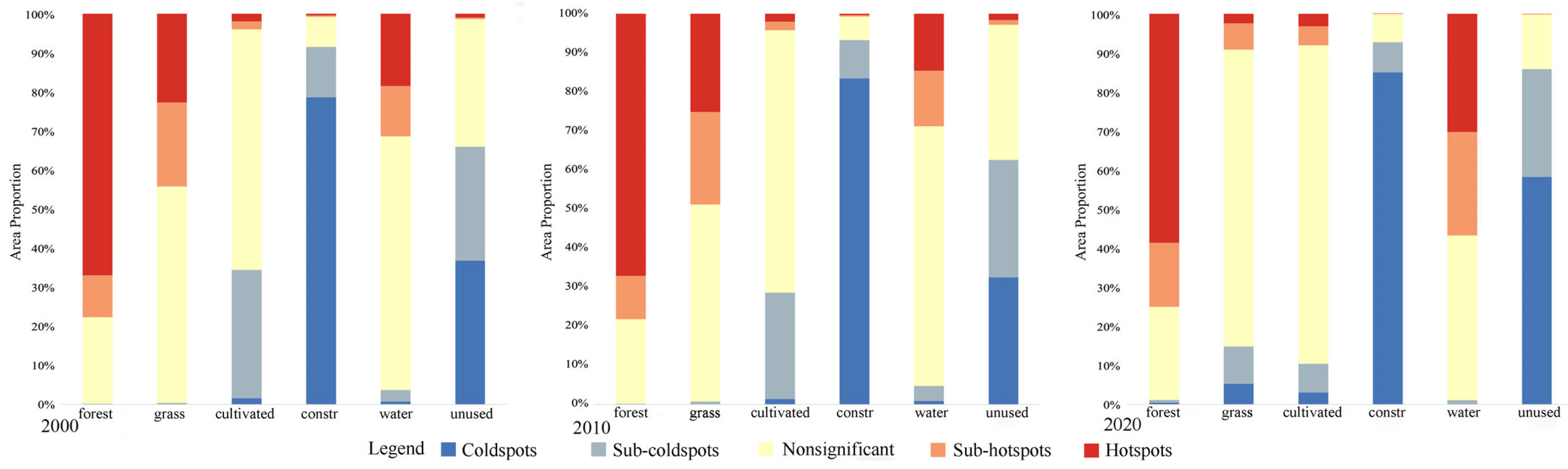
3.3.1. The Heterogeneity of HQ Hotspots in Different Geomorphological Types

The geomorphological types of CMC are complex and diverse, which directly affect the regional ecosystem structure and process and determine the topographic heterogeneity of HQ. The distribution index of HQ hotspots and coldspots in different geomorphological regions can intuitively reflect the topographic heterogeneity. From 2000 to 2020, HQ hotspots always had obvious distribution advantages in mountainous areas (Figure 9), with a distribution index greater than 2.5 and an increasing trend. The distribution index in the trough valley decreased from 1.20 to 0.65, indicating that the distribution of hotspots tended to gather in the mountains. The distribution index of the sub-hotspots in the trough valley, rivers, and mountains was greater than 1, and the distribution advantage in the trough valley decreased significantly, with the distribution index decreasing from 2.04 to 1.42. The coldspots and sub-coldspots had the most obvious distribution advantages in the flat areas, with average distribution indices of 2.60 and 1.09, respectively, followed by the average distribution indices of 1.09 and 1.29 in the hills. In 2020, the sub-coldspots gradually gained the distribution advantage in the trough valley and rivers, with distribution indices of 1.16 and 1.27, respectively. In summary, the HQ hotspots were the most selective to topographic and geomorphic conditions and always concentrated in mountainous areas. On the contrary, flat areas were the main distribution area of the coldspots.

In view of the fact that mountains were always the main distribution areas of the HQ hotspots, the distribution index of the hotspots under different micro-geomorphology types was further calculated to better reveal their micro-topographic heterogeneity. From 2000 to 2020, HQ hotspots had obvious distribution advantages in the top and middle of the mountains (Figure 10), especially in the summits, with an average distribution index of 2.16 but a decreasing trend. The sub-hotspots had a certain distribution advantage in the shoulders, slopes, footslopes, and valleys, and the average distribution index is greater than 1, with minimal variation. The distribution of the coldspots and sub-coldspots had obvious advantages in the ridges and footslopes, and both exhibited a rising trend. In summary, the heterogeneity of HQ at the mountain micro-geomorphology scale was manifested in that the summits were always the hotspots of HQ, and the HQ level in the middle of mountains was relatively high, while the ridges and footslopes were HQ coldspots.

3.3.2. The Heterogeneity of HQ Hotspots in Different Land Use Types

HQ was affected by land use types, so the distribution of HQ hotspots in different land use types had obvious differences. The variation degree of HQ hotspots in different land use types was different.

From the perspective of land use types (Figure 11), the HQ hotspots were mainly composed of forestland, cultivated land, and water areas, and the average proportions of the three land use types were 87.00%, 8.27%, and 3.51%, respectively. With rich biodiversity and strong ecosystem service supply capacity, forestland had a high HQ index and was the dominant distribution area of hotspots. The main composition of the sub-hotspots was the same as that of the hotspots, and the proportion of forestland was as high as 54.47%, followed by cultivated land (32.03%). The total area of the nonsignificant area was the highest, and it was mainly composed of cultivated land, accounting for about 80%. Over the last two decades, the extent of sub-coldspots has decreased greatly. Since the main land use types of the sub-coldspots are cultivated land and construction land, the area of cultivated land had decreased significantly, which was the main reason for the area reduction of the sub-coldspots. The coldspots were mainly composed of construction land, and the area had been increasing continuously in the past 20 years. On the whole, the heterogeneity of HQ hotspots in different land use types mainly showed that the proportion of cultivated land in the sub-coldspots and the nonsignificant area decreased, and the share of construction land within the coldspots and forestland in the sub-hotspots area increased.

According to the area proportion of HQ coldspots and hotspots in each land use type (Figure 12), forestland was the main contributor to the hotspots of HQ. Between the years 2000 and 2020, the HQ hotspots in forestland always dominated, accounting for 66.90%, 67.05%, and 58.61%, respectively. Although the total area of grassland was small, it had a certain contribution to the hotspots. The proportion of hotspots and sub-hotspots in the grassland was 16.76% and 17.31%, respectively. Most of the construction land and unused land were coldspots and sub-coldspots where the HQ index was low. From 2010 to 2020, the proportion of hotspots and sub-hotspots of HQ in water areas increased significantly.

In conclusion, the distribution of HQ coldspots and hotspots in different land use types was different. The construction land was the human activity area, and the HQ was the lowest. The forestland, grassland, and water areas were rich in biodiversity, and the HQ was relatively better because the intensity of human activities was less [29].

3.4. Nonlinear Influence Effects on HQ

The hypothesis test results of the GAM were divided into two parts: the upper part of the table was the parameter results of the linear model, the lower part was the parameter estimates of the nonlinear model, the estimate of the smooth function, and the hypothesis test (

Table 7. Outcomes of GAM hypothesis testing evaluating the relationships between HQ and fixed factors.

Parameter	Parametric Estimate	Std. Error	T-Value	p-Value
Intercept	−0.063560	0.050772	−1.252	0.210631
Cultivated land	0.335495	0.050595	6.631	3.44 × 10−11 ***
Forestland	0.507315	0.050666	10.013	<2 × 10−16 ***
Grassland	0.432428	0.051877	8.336	<2 × 10−16 ***
Water areas	0.391870	0.051363	7.629	2.49 × 10−14 ***
Construction land	0.286391	0.050772	5.641	1.72 × 10−8 ***
Unused land	0.369158	0.097053	3.804	0.000143 ***
Flat areas	−0.010782	0.006663	−1.618	0.105640
Top-slope	0.101374	0.008469	11.969	<2 × 10−16 ***
Mid-slope	0.129301	0.005969	21.663	<2 × 10−16 ***
Footslope	0.102275	0.007488	13.658	<2 × 10−16 ***
Hills	0.031711	0.012185	2.602	0.009265 **
Trough valley	−0.032755	0.005250	−6.239	4.51 × 10−10 ***
River way	0.102973	0.018745	5.493	4.00 × 10−8 ***
Multi-center groups strategies	−0.146346	0.017455	−8.384	<2 × 10−16 ***
Four parallel mountains’ developments and controls	0.054770	0.048296	1.134	0.000212 ***
Ecological redlines	0.056627	0.004662	12.146	<2 × 10−16 ***
Beautiful landscape city planning	0.036629	0.004539	8.070	7.51 × 10−16 ***
Smooth terms	Estimated degree of freedom	Reference degree of freedom	F-value	p-value
s(DEM)	7.953	9.042	9.540	<2 × 10−16 ***
s(Slope)	1.284	1.518	0.414	0.733
s(Aspect)	4.716	5.610	1.817	0.099
s(TPI)	2.000	2.320	48.748	<2 × 10−16 ***
s(TNI)	3.463	3.846	22.377	<2 × 10−16 ***
s(NDVI)	1.989	2.000	172.510	<2 × 10−16 ***
s(NPP)	2.971	2.999	120.121	<2 × 10−16 ***
s(Pre)	4.643	4.945	45.655	<2 × 10−16 ***
s(OC)	2.950	2.998	36.371	<2 × 10−16 ***
s(Dis_forest)	2.986	3.000	159.328	<2 × 10−16 ***
s(Dis_grass)	1.979	2.000	25.845	<2 × 10−16 ***
s(Dis_cult)	7.814	7.987	73.608	<2 × 10−16 ***
s(Dis_water)	3.833	4.442	5.814	8.57 × 10−5 ***
s(Dis_cons)	2.892	3.000	114.695	<2 × 10−16 ***
s(POP)	2.707	2.941	17.746	<2 × 10−16 ***
s(GDP)	2.832	2.980	15.490	<2 × 10−16 ***

The statistical significance levels were very significant (** p < 0.01), and extremely significant (*** p < 0.001). Pre: precipitation; OC: soil organic matter content; Dis_forest: distance to forestland; Dis_grass: distance to grass; Dis_cult: distance to cultivated land; Dis_water: distance to water areas; Dis_con: distance to construction land.

). The results showed that except for flat areas, land use type, landform type, and policy implementation had significant statistical significance with HQ. Specifically, forestland, grassland, and water areas exhibited a strong positive association with HQ, with parameter estimates of 0.507, 0.432, and 0.392, respectively. A strong positive relationship was observed between HQ and the mid-slope, with a parameter estimate of 0.130. There was a significant negative correlation with the trough valley, and the parameter estimate was 0.033. The river way can maintain a certain level of biodiversity, and the parameter estimate was 0.103. The implementation of ecological protection policies positively influenced HQ.

Among the smoothing effect terms, except for slope and aspect, all environmental variables had significant statistical significance on the HQ. The accepted probabilities of different environmental variables in model fitting can reflect their importance to HQ. According to the F-value, it could be seen that the NDVI was the most important influencing factor affecting HQ, with an F-value of 172.510. Followed by the dis_forest, NPP, the dis_cons, the dis_cult, TPI, and so on.

Smoothers describe HQ as a function of the respective predictor (lines) along with their 95% confidence intervals (gray shading) and partial residuals. In the graph of the influence effects of environmental factors on HQ (Figure 13), the X axis represents environmental factors, and the Y axis represents partial residuals. The number in the y-axis label was the estimated degrees of freedom (edf) of the smoothers function. When edf was close to 1, it showed a linear relationship, and when edf was greater than 1, it was nonlinear.

There were extremely significant nonlinear relationships between HQ and environmental factors, in which the HQ initially declined with rising elevation, followed by a pattern of fluctuating increases. And HQ initially declined but later improved as NDVI, TNI, and soil organic matter content increased. The pattern of HQ exhibited an M-shaped undulation in response to the aspect, reaching its zenith around 100° and 275°. The relationship between HQ and TPI, when represented by a smoothed curve, assumed a V-shape, with the HQ reaching its nadir at a TPI value of 0. There was a positive correlation between HQ and NPP. And HQ referred to a fluctuating downward trend as precipitation increased. The farther the distance to forestland, the lower the HQ. As the distance to grassland increased, the HQ decreased first and then increased. The HQ showed a multi-peak fluctuation trend with the increase in the distance to cultivated land, which was closely related to the mosaic distribution of striped parallel mountains and valleys cultivated land, as well as the complex combination of landforms such as anticlinal mountains and the trough valley cultivated land developed on the top. The HQ showed a fluctuating increased trend with the increase in the distance to construction land and waters, and the fluctuation of HQ from construction land was greater. The HQ tended to decrease with the increase in population density and GDP.

4. Discussion

4.1. Optimal Assessment of HQ Considering Mountain Micro-Topographic Characteristics

Topography is the dominant factor affecting the HQ of mountain cities. For example, topographic fluctuation directly affects the distribution of water and temperature. Soil erosion and accumulation are greatly affected by topographic slope. Terrain can also block or guide the wind direction, affecting wind speed and thus affecting the growth of vegetation and the habitat of animals. In addition, the terrain directly determines the biological migration path and affects biological communication [30]. At present, while numerous studies have explored the influence of topography on HQ [31], limited research has integrated mountain micro-geomorphology to optimize HQ assessment. In fact, different types of micro-geomorphology affect the living space, water source, food, and natural enemies of organisms, create favorable living environments for particular species, and jointly maintain the diversity of mountain ecosystems [32]. In this paper, the HQ hotspots always had obvious distribution advantages in the summits, and the distribution index of the sub-hotspots in the shoulders, footslopes, and valleys was also greater than 1. Relevant studies had shown that the top of mountains was usually more open, which was conducive to biological migration and foraging. In addition, the summits are a biological refuge, providing living space for alpine species and endemic species [33]. The shoulder is located between the ridge and the slope, with a gentle slope and relatively fertile soil. The open living space on the shoulder provides suitable living conditions for a variety of plants and animals [34]. Similarly, the footslope is a transition zone between mountains and plains, providing a rich ecological niche and supporting a high level of biodiversity [35]. The valley can provide relatively moist habitats for organisms, and it is an important habitat for aquatic and wet organisms, as well as an important route for plant spread and animal migration [36].

In this study, the mountain forestland was subdivided into five types according to the mountain micro-topographic position, and the HQ assessment was optimized by calculating the variation coefficient of the RVI based on UAV multispectral image acquisition and processing. HQ refers to the suitability of environmental conditions for the survival and reproduction of organisms in a specific area, which directly determines the regional biodiversity [14]. Based on the spectral variation hypothesis, the spectral reflectance characteristics of plant communities are closely related to biodiversity, and the variation characteristics of vegetation indices are commonly used to monitor tree species diversity. The standard deviation, variance, and variation coefficient of NDVI are often used to monitor and invert biodiversity [37]. Although NDVI is widely used, it has certain limitations. NDVI values are easily saturated in areas with high vegetation coverage, and soil and canopy background noise can lead to uncertainty of vegetation index [38]. Many scholars have also explored the application of RVI and difference vegetation index (DVI) in biodiversity inversion [39]. Related studies have shown that the variation characteristics of the RVI had better comprehensive explanatory power for tree species diversity than that of NDVI [40].

4.2. The Analysis of the Spatiotemporal Change in HQ in the CMC

Between 2000 and 2020, the HQ in the CMC exhibited a general upward trend, with a decreasing trend in the urban central areas and an increasing trend in the periphery. This was mainly influenced by two factors: urban development and the implementation of ecological protection policies.

Amid ongoing urbanization and escalating human activities, the dual processes of new area expansion and old area renewal, coupled with improving infrastructure [41], resulted in the occupation of 752.64 km² of cultivated land and an increase in construction land by 776.93 km². This directly led to the expansion of HQ coldspots from 412.58 km² to 1042.60 km² (Figure 14). Following Chongqing’s designation as a centrally administered municipality in 1997, a large number of cross-river bridges and mountain tunnels were constructed. The original urban groups in the central region were gradually connected and gradually developed, crossing Zhongliang Mountain to the west and breaking through Tongluo Mountain and Nanshan to the east. In 2000, the Eastern Tea Garden New Area was approved for establishment. Chongqing Jiangbei International Airport were expanded in 2001 and 2008. In 2003, the western university area was approved for construction. In 2009, the entire Ring Expressway was opened to traffic. In 2010, Liangjiang New Area was established as the first national level of inland development and opening up new areas in China [42]. The urbanization rate in the Yuzhong district was as high as 100%. The high-density population, high-intensity production, and living interference had led to a lower level of regional HQ. The overall HQ of the nine administrative districts was showing an increasing trend. Jiangbei district showed the smallest increase, with an HQ increase of only 0.090. This was closely tied to the rapid development and heightened urbanization of the Liangjiang New Area [43]. The specific urban spatial layout planning made the urban groups gradually connect seamlessly, and the infrastructure was gradually improved. According to the overall urban planning of Chongqing from 2007 to 2020, the Chongqing main city had formulated a “multi-center groups development strategy”. This strategy planned the 16 urban groups in Yuzhong, Dayangshi, Dadukou, Shapingba, Guanyin Bridge–Renhe, Dazhulin–Lijia, Caijia, Lianglu, Tangjiatuo, Nanping, Lijiatuo–Yudong, Beibei, Xiyong, Xipeng, Yuzui, and Tea Garden–Lujiao. The transportation network, population density, and social economic development within each group were becoming increasingly developed [44]. In the past 20 years, the total population has increased by 1.73 million, and the GDP has increased nearly 16-fold (Figure 15). The high-density population and high-intensity production had led to the urbanization rate increasing substantially from 50.26% to 93.54% and a decrease in local HQ.

On the other hand, as ecological protection efforts intensified, the overall HQ index in CMC improved despite localized declines in certain areas. From 2010 to 2020, the HQ showed an increasing trend, and the hotspots increased from 838.14 km² to 1086.16 km² (Figure 14). The improvement in HQ was mainly due to the strict and effective ecological protection work over the years. The overall urban planning of Chongqing emphasized the protection of the urban landscape and ecological environment, strengthening the integration and construction of suburban and rural residential areas, improving the quality of the living environment, coordinating the promotion of ecological construction, environmental protection, and green space system construction [45]. In 2008, the ecological function zoning of Chongqing was promulgated, Beibei, Banan, and Yubei districts were identified as important ecological barriers in the metropolitan. Most of the areas in the three administrative districts were less disturbed by human activities, had good vegetation coverage, and maintained a high level of HQ. In 2016, the beautiful landscape city planning in CMC was formulated. Through a comprehensive analysis of the natural background conditions of mountains, waters, and green, the veins of the mountain system, water system, and green system were clarified, and the integrated development planning strategy of landscape city was defined, which integrated ecological protection and urban development. To rigorously safeguard the critical ecological barrier areas of the Four Mountains, the vital conservation areas of the Yangtze and Jialing River basins, and the mountain and green space systems with significant ecological functions, the 1736.7 km² areas were designated as ecological protection redline areas in the CMC in 2016. In addition, the strict management and ecological protection of nature reserves and forest parks at all levels provided suitable habitats for living, survival, and reproduction [46]. Therefore, the improvement of HQ in Banan, Beibei, and Yubei districts was the most obvious.

4.3. Nonlinear Influencing Mechanism of HQ Under Complex Landscape City

Previous studies have neglected the nonlinear mechanism of HQ caused by the combination of landscape patterns and landforms in mountain cities. The GAM is capable of capturing both linear relationships and, through its non-parametric smoothing function, adeptly modeling nonlinear interactions between independent and dependent variables [47]. The model is conducive to the scientific identification and analysis of the characteristics of the dominant influence factors and their responses [48], which has a relatively strong ability to explain the spatiotemporal differentiation of HQ under the complex landscape city pattern in the CMC.

The HQ initially declined but then exhibited a fluctuating rise as elevation increased (Figure 13), which was mainly because the lowest altitude areas in CMC were mainly composed of rivers, lakes, and other waters. The water areas were very important for aquatic animals and plants, such as swimming birds that like to feed and roost in water, and water is also an important foraging ground for wading birds [49]. The high-altitude areas belong to parallel mountain areas with high vegetation coverage, and the change in topographic factors regulates various resource gradients such as solar radiation and soil [50], creating a suitable habitat for a variety of animals and plants. With the increase in slope, the topography of mountain areas becomes more complex, human activities decrease, and habitat types are diverse, making mountain areas an important shelter for animals and plants. The HQ index showed an M-shaped fluctuation trend with aspect, which was influenced by the trend of parallel folded mountains from northeast to southwest, resulting in a higher area proportion of forestland on the eastern slope and the western slope and a relatively higher HQ. Areas with higher or lower TPI values, indicating proximity to ridges or valleys, tended to exhibit higher HQ.

In the CMC, forests with a certain quality and scale composed of forestland were mainly located in the parallel mountain areas. Affected by topographic factors, the horizontal and vertical structures inside the forests were relatively complete, and the habitat types were diverse [51]. The different resource utilization strategies of plants inhibited the competitive exclusion effect of communities [52], led to the ecological niche differentiation of different plants, and provided suitable conditions for the survival and reproduction of various plants and animals. Therefore, the further the distance to the forestland, the HQ index would decrease. The occurrence of a single wave crest was related to the ability of the waters to maintain a certain level of biodiversity.

There was a positive correlation between HQ and NPP, and HQ showed a trend of fluctuation decreases with the increase in Pre. There was a trend of multi-wave peak fluctuation between HQ and the distance to cultivated land, which was closely related to the mosaic distribution of long strip parallel mountains and valleys cultivated land, and the complex geomorphologic combination of the anticlinal mountain range and the trough valley cultivated land developed on the top. The multi-center groups’ urban development pattern across rivers and mountains had resulted in a fluctuating rise in HQ with greater distance from construction land. Simultaneously, as POP and GDP grew, the intensifying influence of human activities contributed to a decline in HQ.

4.4. Limitations and Future Works

The innovation of this study was to consider the mountain micro-topographic characteristics and to obtain the RVI variation coefficient of forestland in different mountain micro-topographic positions based on the UAV multispectral data collection and procession so as to optimize the habitat suitability parameters of the InVEST model. However, this study only modified the model for mountainous areas and only carried out field investigation with Jinyun Mountain as an example. In the future, more comprehensive field investigations should be carried out to fully consider the internal mechanisms of HQ, and model parameter localization should be strengthened to assess HQ more accurately. In addition, although the HQ obtained by the InVEST model can be used as a proxy for the ability of the ecosystem to provide conditions appropriate for individual survival, reproduction, and population persistence, the model parameter setting was still somewhat subjective, and the model does not adequately take into account the actual species distribution. How to further combine remote sensing, geographic information, and species distribution information to effectively and comprehensively evaluate HQ by coupling species potential distribution model will be the focus of future research work. Furthermore, it is also important to further reveal the influence intensity and response mode of the interaction of natural, social, and policy-influencing factors on the spatial differentiation of HQ.

5. Conclusions

This research comprehensively considered the mountainous micro-geomorphology characteristics to optimize and evaluate the spatiotemporal patterns of HQ in the CMC between 2000 and 2020 based on the HQ module of the InVEST model. Methods such as least-squares trend analysis, hotspot analysis, and GAM were used to explore the spatiotemporal variation characteristics of HQ, clarify the spatiotemporal differentiation of HQ hotspots, and explore the nonlinear influencing mechanism of HQ, and the following findings were obtained:

(1)

The overall HQ in CMC exhibited significant spatial variability. High-value HQ areas were mainly concentrated in mountainous areas such as Jinyun Mountain, Zhongliang Mountain, Tongluo Mountain, and Mingyue Mountain, while the HQ in the urban central areas was lower. From 2000 to 2020, on the one hand, the urbanization process continued to advance, and the interference from human activities continued to increase. On the other hand, ecological protection has been strengthened. While the HQ index level in some areas had decreased, the overall HQ level in CMC had improved. Beibei, Banan, and Yubei districts had the highest average HQ level, while Yuzhong district had the lowest;

(2)

HQ hotspots were mainly distributed in parallel mountain areas and ran through the entire study area with a trend from northeast to southwest. Coldspots were mainly distributed in the urban central areas in the central and western parts of the study area. The area of HQ hotspots showed an overall increasing trend, which was mainly due to strict ecological protection work in recent years. With the expansion of construction land, the total area of coldspots had increased rapidly. The HQ hotspots had the highest distribution advantage in mountainous areas, and the distribution index was greater than 2.5, indicating that the mountainous areas were the concentrated distribution areas of HQ hotspots. Specifically, the heterogeneity of HQ at the mountain micro-geomorphology scale was manifested in that the summits were always the hotspots of HQ, with an average distribution index of 2.16. In terms of the composition of land use types, the hotspots and sub-hotspots primarily consisted of forestland, cultivated land, and waters, of which the average proportion of forestland was 87.00% and 54.47%, respectively. Forestland was also a major contributor to HQ hotspots. Over the past two decades, HQ hotspots in forestland have always dominated, accounting for 66.90%, 67.05%, and 58.61%, respectively;

(3)

HQ was comprehensively affected by a combination of diverse factors, including natural environmental conditions, socio-economic elements, and the execution of policies. Among them, the NDVI and the distance to forestland had very significant nonlinear relationships with HQ. It was mainly related to the mosaic distribution of long strip parallel mountains and valleys cultivated land in CMC, as well as the complex geomorphologic combination of the anticlinal mountains and the trough valley cultivated land developed on the top.

In conclusion, this study revealed the spatiotemporal evolution of urban HQ and its nonlinear influencing mechanism in the CMC, which provided important references for regional ecological protection and urban sustainable development.

References

1. Huang, Z.; Bai, Y.; Alatalo, J.M.; Yang, Z. Mapping biodiversity conservation priorities for protected areas: A case study in Xishuangbanna tropical area, China. Biol. Conserv. 2020, 249, 108741. [Google Scholar] [CrossRef]
2. Peng, J.; Tian, L.; Liu, Y.; Zhao, M.; Hu, Y.; Wu, J. Ecosystem services response to urbanization in metropolitan areas: Thresholds identification. Sci. Total Environ. 2017, 607–608, 706–714. [Google Scholar] [CrossRef]
3. Convention on Biological Diversity (CBD). Available online: https://www.cbd.int/sp/targets/ (accessed on 30 October 2023).
4. Convention on Biological Diversity (CBD). Available online: https://www.cbd.int/meetings/COP-15 (accessed on 30 October 2023).
5. Jiang, B.; Bai, Y.; Wong, C.P.; Xu, X.; Alatalo, J.M. China’s ecological civilization program–Implementing ecological redline policy. Land Use Policy 2019, 81, 111–114. [Google Scholar] [CrossRef]
6. Guo, K.; Niu, X.; Wang, B.; Xu, T.Y.; Ma, X. Dynamic changes in habitat quality and the driving mechanism in the Luoxiao mountains area from 1995 to 2020. Ecosyst. Health Sust. 2023, 9, 0039. [Google Scholar] [CrossRef]
7. Louis, V.; Page, S.E.; Tansey, K.J.; Jones, L.; Bika, K.; Balzter, H. Tiger habitat quality modelling in Malaysia with Sentinel-2 and InVEST. Remote Sens. 2024, 16, 284. [Google Scholar] [CrossRef]
8. Zhang, T.; Gao, Y.; Li, C.; Xie, Z.; Chang, Y.; Zhang, B. How human activity has changed the regional habitat quality in an eco-economic zone: Evidence from Poyang Lake Eco-Economic Zone, China. Int. J. Environ. Res. Public Health 2020, 17, 6253. [Google Scholar] [CrossRef] [PubMed]
9. Wang, B.; Cheng, W. Effects of land use/cover on regional habitat quality under different geomorphic types based on InVEST model. Remote Sens. 2022, 14, 1279. [Google Scholar] [CrossRef]
10. Li, X.; Cheng, S.; Wang, Y.; Zhang, G.; Zhang, L.; Wu, C. Future land use spatial conflicts and habitat quality impacts based on SSPs-RCPs Scenarios—Qin-Ba Mountain City. Land 2023, 12, 1708. [Google Scholar] [CrossRef]
11. Wei, W.; Bao, Y.; Wang, Z.; Chen, X.; Luo, Q.; Mo, Y. Response of habitat quality to urban spatial morphological structure in multi-mountainous city. Ecol. Indic. 2023, 146, 109877. [Google Scholar] [CrossRef]
12. Bai, L.; Xiu, C.; Feng, X.; Liu, D. Influence of urbanization on regional habitat quality: A case study of Changchun City. Habitat. Int. 2019, 93, 102042. [Google Scholar] [CrossRef]
13. Bi, M.; Zhong, Y.; Xiao, Z.; Feng, X.; Ma, H. Spatial and temporal change of habitat quality of Poyang Lake Basin in China at small watershed scale and its multidimensional response to landscape pattern. Chin. Geogr. Sci. 2023, 33, 565–582. [Google Scholar] [CrossRef]
14. Chen, C.; Liu, J.; Bi, L. Spatial and temporal changes of habitat quality and its influential factors in China based on the InVEST model. Forests 2023, 14, 374. [Google Scholar] [CrossRef]
15. Hu, J.; Zhang, J.; Li, Y. Exploring the spatial and temporal driving mechanisms of landscape patterns on habitat quality in a city undergoing rapid urbanization based on GTWR and MGWR: The case of Nanjing, China. Ecol. Indic. 2022, 143, 109333. [Google Scholar] [CrossRef]
16. Jia, C.; Li, Z.; Yang, X.; Liu, H.; Yang, X. The spatiotemporal evolution characteristics and influencing factors of habitat quality in the typical region of the Lunan Economic Belt: A case study of Donggang District, Rizhao. Environ. Monit. Assess. 2024, 196, 1074. [Google Scholar] [CrossRef] [PubMed]
17. Xu, J.; Ling, Y.; Sun, Y.; Jiang, Y.; Shen, R.; Wang, Y. How do different processes of habitat fragmentation affect habitat quality?–Evidence from China. Ecol. Indic. 2024, 160, 111880. [Google Scholar] [CrossRef]
18. Mondal, I.; Naskar, P.K.; Alsulamy, S.; Jose, F.; Hossain, S.K.A.; Mohammad, L.; De, T.K.; Khedher, K.M.; Salem, M.A.; Benzougagh, B.; et al. Habitat quality and degradation change analysis for the Sundarbans mangrove forest using invest habitat quality model and machine learning. Environ. Dev. Sustain. 2024, 1–26. [Google Scholar] [CrossRef]
19. Liu, S.; Liao, Q.; Xiao, M.; Zhao, D.; Huang, C. Spatial and temporal variations of habitat quality and its response of landscape dynamic in the Three Gorges Reservoir Area, China. Int. J. Environ. Res. Public Health 2022, 19, 3594. [Google Scholar] [CrossRef]
20. Chongqing Bureau of Statistics; China’s National Bureau of Statistics. Chongqing Statistical Yearbook; China Statistics Press: Beijing, China, 2021. [Google Scholar]
21. Tang, Z.L.; Fu, M.; Wang, Y.T.; Zhao, Y.H. Spatial characteristics of industrial economic location and its formation in Chongqing, China. Front. Environ. Sci. 2023, 11, 1115067. [Google Scholar] [CrossRef]
22. Wang, F.; Yuan, X.; Zhou, L.; Liu, S.; Zhang, M.; Zhang, D. Detecting the complex relationships and driving mechanisms of key ecosystem services in the Central Urban Area Chongqing Municipality, China. Remote Sens. 2021, 13, 4248. [Google Scholar] [CrossRef]
23. Jasiewicz, J.; Stepinski, T.F. Geomorphons—A pattern recognition approach to classification and mapping of landforms. Geomorphology 2013, 182, 147–156. [Google Scholar] [CrossRef]
24. Deng, J.; Cheng, W.; Liu, Q.; Jiao, Y.; Liu, J. Morphological differentiation characteristics and classification criteria of lunar surface relief amplitude. J. Geogr. Sci. 2022, 32, 2365–2378. [Google Scholar] [CrossRef]
25. Libohova, Z.; Winzeler, H.E.; Lee, B.; Schoeneberger, P.J.; Datta, J.; Owens, P.R. Geomorphons: Landform and property predictions in a glacial moraine in Indiana landscapes. Catena 2016, 142, 66–76. [Google Scholar] [CrossRef]
26. Fang, C.S.; Wang, L.Y.; Li, Z.Q.; Wang, J. Spatial characteristics and regional transmission analysis of PM2.5 pollution in northeast China, 2016-2020. Int. J. Environ. Res. Public Health 2021, 18, 12483. [Google Scholar] [CrossRef]
27. Zuur, A.F.; Ieno, E.N.; Elphick, C.S. A protocol for data exploration to avoid common statistical problems. Methods Ecol. Evol. 2010, 1, 3–14. [Google Scholar] [CrossRef]
28. Hastie, T.; Tibshirani, R. Generalized Additive Models. In Wiley StatsRef: Statistics Reference Online; CRC Press: Boca Raton, FL, USA, 2014. [Google Scholar]
29. Xiao, P.; Zhou, Y.; Li, M.; Xu, J. Spatiotemporal patterns of habitat quality and its topographic gradient effects of Hubei province based on the InVEST model. Environ. Dev. Sustain. 2023, 25, 6419–6448. [Google Scholar] [CrossRef]
30. Swanson, F.J.; Kratz, T.K.; Caine, N.; Woodmansee, R.G. Landform effects on ecosystem patterns and processes: Geomorphic features of the earth’s surface regulate the distribution of organisms and processes. BioScience 1988, 38, 92–98. [Google Scholar] [CrossRef]
31. Huang, H.; Xiao, Y.; Ding, G.; Liao, L.; Yan, C.; Liu, Q.; Gao, Y.; Xie, X. Comprehensive evaluation of island habitat quality based on the Invest model and terrain diversity: A case study of Haitan Island, China. Sustainability 2023, 15, 11293. [Google Scholar] [CrossRef]
32. Liu, Y.; Du, J.; Xu, X.; Kardol, P.; Hu, D. Microtopography-induced ecohydrological effects alter plant community structure. Geoderma 2020, 362, 114119. [Google Scholar] [CrossRef]
33. Zhang, L.; Wang, J. Mountain biodiversity, species distribution and ecosystem functioning in a changing world. Diversity 2023, 15, 799. [Google Scholar] [CrossRef]
34. Cho, K.H.; Hong, S.K.; Cho, D.-S. Ecological role of mountain ridges in and around gwangneung royal tomb forest in central Korea. J. Plant Biol. 2008, 51, 387–394. [Google Scholar] [CrossRef]
35. Jiang, Y.; Kang, M.; Zhu, Y.; Xu, G. Plant biodiversity patterns on Helan Mountain, China. Acta Oecologica 2007, 32, 125–133. [Google Scholar] [CrossRef]
36. Wierzcholska, S.; Dyderski, M.K.; Pielech, R.; Gazda, A.; Smoczyk, M.; Malicki, M.; Horodecki, P.; Kamczyc, J.; Skorupski, M.; Hachułka, M.; et al. Natural forest remnants as refugia for bryophyte diversity in a transformed mountain river valley landscape. Sci. Total Environ. 2018, 640–641, 954–964. [Google Scholar] [CrossRef]
37. Krishnaswamy, J.; Bawa, K.S.; Ganeshaiah, K.N.; Kiran, M.C. Quantifying and mapping biodiversity and ecosystem services: Utility of a multi-season NDVI based Mahalanobis distance surrogate. Remote Sens. Environ. 2009, 113, 857–867. [Google Scholar] [CrossRef]
38. Wang, Z.; Liu, C.; Huete, A. From AVHRR-NDVI to MODIS-EVI: Advances in vegetation index research. Acta Ecol. Sin. 2003, 23, 979–987. [Google Scholar]
39. Sun, G.; Jiao, Z.; Zhang, A.; Li, F.; Fu, H.; Li, Z. Hyperspectral image-based vegetation index (HSVI): A new vegetation index for urban ecological research. Int. J. Appl. Earth Obs. Geoinf. 2021, 103, 102529. [Google Scholar] [CrossRef]
40. Madonsela, S.; Cho, M.A.; Ramoelo, A.; Mutanga, O. Remote sensing of species diversity using Landsat 8 spectral variables. ISPRS J. Photogramm. Remote Sens. 2017, 133, 116–127. [Google Scholar] [CrossRef]
41. Wang, S.; Lu, F.; Wei, G. Direct and spillover effects of urban land expansion on habitat quality in Chengdu-Chongqing urban agglomeration. Sustainability 2022, 14, 14931. [Google Scholar] [CrossRef]
42. Ma, T.; Liu, R.; Li, Z.; Ma, T. Research on the evolution characteristics and dynamic simulation of habitat quality in the southwest mountainous urban agglomeration from 1990 to 2030. Land 2023, 12, 1488. [Google Scholar] [CrossRef]
43. Zhang, Y.; Li, Y.; Chen, Y.; Liu, S.; Yang, Q. Spatiotemporal heterogeneity of urban land expansion and urban population growth under new urbanization: A case study of Chongqing. Int. J. Environ. Res. Public Health 2022, 19, 779. [Google Scholar] [CrossRef]
44. Zong, H.; Yu, X. Urbanization of Chongqing municipality: Regional contributions and influencing mechanisms. Sustainability 2024, 16, 3734. [Google Scholar] [CrossRef]
45. Liu, Y.; Zhou, T.; Yu, W. Analysis of changes in ecological environment quality and influencing factors in Chongqing based on a remote-sensing ecological index mode. Land 2024, 13, 227. [Google Scholar] [CrossRef]
46. Wang, S.; Tian, M.; Ding, Q.B.; Shao, H.Y.; Xia, S.Y. Study on coupling coordination degree of urbanization and ecological environment in Chengdu-Chongqing economic circle from 2002 to 2018. Environ. Sci. Pollut. Res. 2024, 31, 3134–3151. [Google Scholar] [CrossRef] [PubMed]
47. Shen, Z.; Yang, Y.; Ai, L.; Yu, C.; Su, M. A hybrid CART-GAMs model to evaluate benthic macroinvertebrate habitat suitability in the Pearl River Estuary, China. Ecol. Indic. 2022, 143, 109368. [Google Scholar] [CrossRef]
48. Alahuhta, J.; Ala-Hulkko, T.; Tukiainen, H.; Purola, L.; Akujärvi, A.; Lampinen, R.; Hjort, J. The role of geodiversity in providing ecosystem services at broad scales. Ecol. Indic. 2018, 91, 47–56. [Google Scholar] [CrossRef]
49. Schwentner, M.; Timms, B.V.; Richter, S. Flying with the birds? Recent large-area dispersal of four Australian Limnadopsis species (Crustacea: Branchiopoda: Spinicaudata). Ecol. Evol. 2012, 2, 1605–1626. [Google Scholar] [CrossRef]
50. Poulos, H.M.; Camp, A.E. Topographic influences on vegetation mosaics and tree diversity in the Chihuahuan Desert Borderlands. Ecology 2010, 91, 1140–1151. [Google Scholar] [CrossRef]
51. Takyu, M.; Aiba, S.I.; Kitayama, K. Effects of topography on tropical lower montane forests under different geological conditions on Mount Kinabalu, Borneo. Plant Ecol. 2002, 159, 35–49. [Google Scholar] [CrossRef]
52. Balvanera, P.; Aguirre, E. Tree diversity, environmental heterogeneity, and productivity in a Mexican Tropical Dry Forest. Biotropica 2006, 38, 479–491. [Google Scholar] [CrossRef]
Figure 1. Geographical position and digital elevation model of the Chongqing main city.
Sustainability 17 01515 g001
Figure 2. Topographic and geomorphic division of CMC.
Sustainability 17 01515 g002
Figure 3. Topographic and geomorphologic characteristics of CMC.
Sustainability 17 01515 g003
Figure 4. Micro-topographic division of mountainous area in CMC.
Sustainability 17 01515 g004
Figure 5. Micro-topographic characteristics of mountainous area in CMC.
Sustainability 17 01515 g005
Figure 6. HQ spatiotemporal change trend characteristic.
Sustainability 17 01515 g006
Figure 7. HQ index and its changes in different administrative districts.
Sustainability 17 01515 g007
Figure 8. Spatiotemporal differentiation of coldspots and hotspots of HQ.
Sustainability 17 01515 g008
Figure 9. Distribution index of HQ coldspots and hotspots on different landforms.
Sustainability 17 01515 g009
Figure 10. Distribution index of HQ coldspots and hotspots on different micro-geomorphology types.
Sustainability 17 01515 g010
Figure 11. Composition of land use types in HQ coldspots and hotspots. Note: Construction land (constr). The same is true below.
Sustainability 17 01515 g011
Figure 12. Area proportion of HQ coldspots and hotspots in different land use types.
Sustainability 17 01515 g012
Figure 13. Influence effects of various environmental factors on HQ.
Sustainability 17 01515 g013
Figure 14. The area changes of HQ hotspots and coldspots.
Sustainability 17 01515 g014
Figure 15. Changes in population, GDP, and urbanization rate from 2000 to 2020 in CMC.
Sustainability 17 01515 g015