
Optimal Electric Bus Charging Scheduling with Multiple Vehicle and Charger Types Considering Compatibility


Abstract
:1. Introduction
Contributions
- (i)
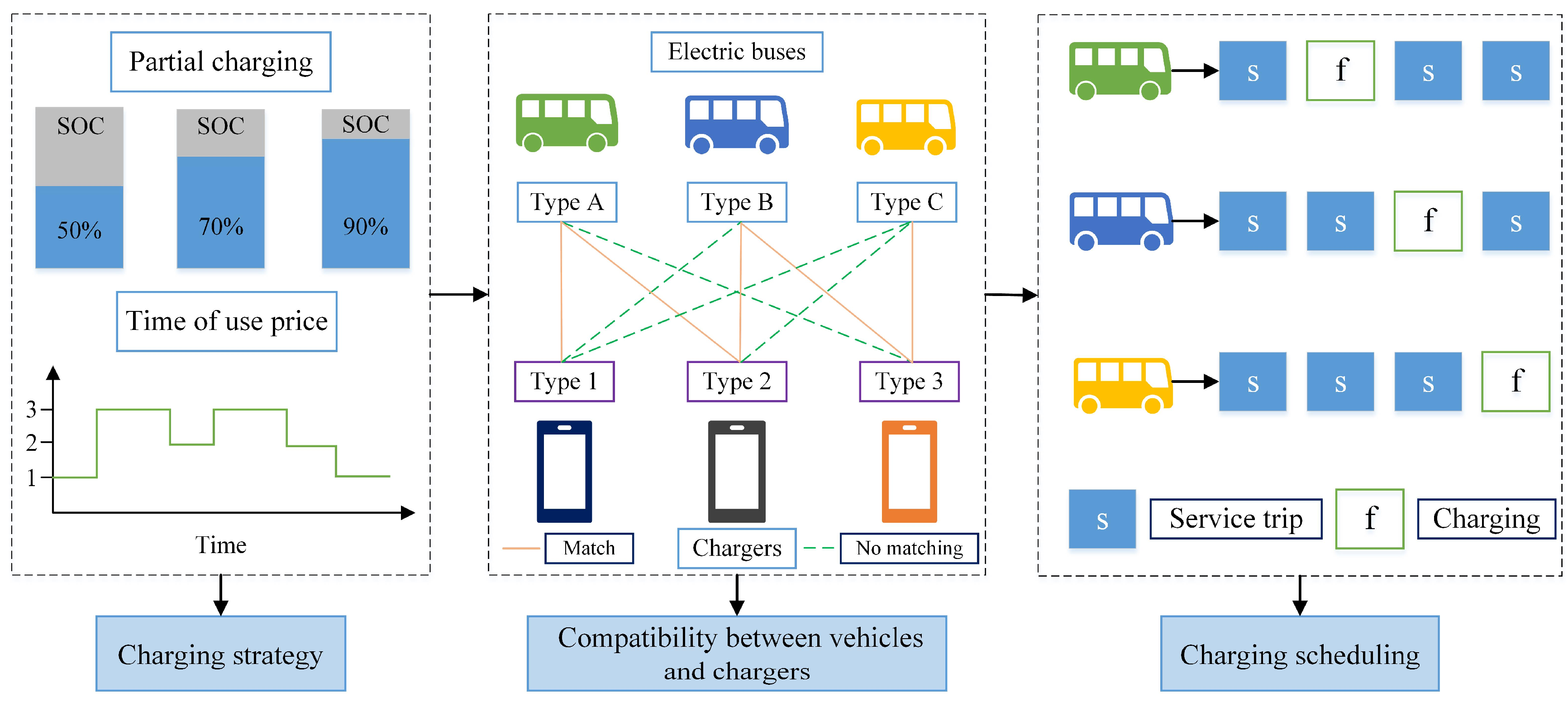
- A joint optimization model of charging infrastructure, fleet composition, and charging scheduling is proposed, and multiple types of vehicles and chargers are considered.
- (ii)
- The compatibility of vehicles and chargers is optimized to reduce the total system costs.
- (iii)
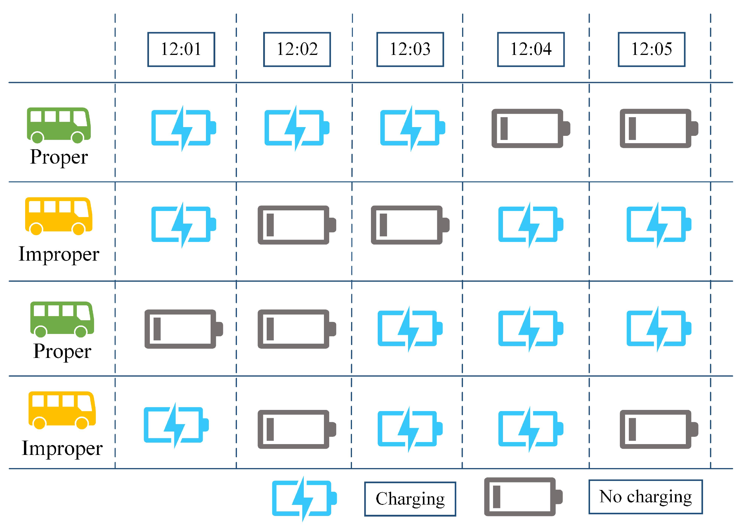
- A partial charging strategy, including ToU electricity price and charging continuity, is proposed, which aligns more with BEB transit operation and practice.From a methodological perspective, the study contributes to the following:
- (iv)
- By model linearization, the proposed model integrates constraints of partial charging strategies, minimum charging time, and continuity requirements under a series of state-of-charge (SoC) updating functions without quadratic terms.
- (v)
- A column generation algorithm is designed to obtain the optimal solution, and a comparison is conducted between the CG algorithm and the CPLEX solver (Version: 12.8.0).
- (vi)
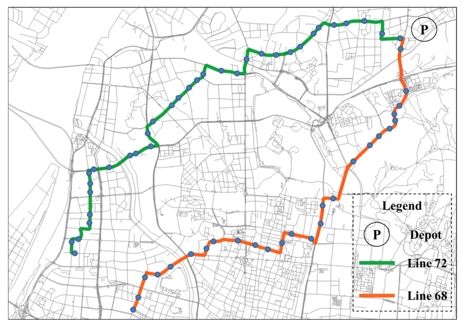
- Two BEB routes are used as case studies to validate the effectiveness of the proposed model and algorithm. Additionally, a sensitivity analysis is performed under various parameter combinations.
2. Literature Review
3. Methodology
3.1. Problem Description
3.2. Model Development
3.2.1. Purchase Costs of Chargers
3.2.2. Fleet Composition Costs
3.2.3. Electricity Costs
3.2.4. Objective Function and Constraints
4. Solution Algorithm
4.1. Master Problem Formulation
4.2. Reduced Cost Calculation
4.3. Subproblems with Math Programming
5. Case Study
Experimental Background
6. Results
6.1. Comparison Between CPLEX and CG Algorithm
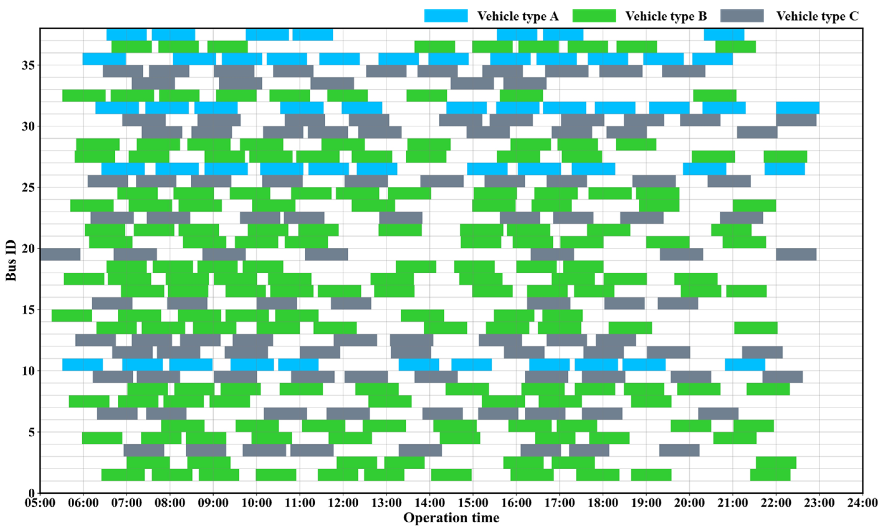
6.2. Numerical Results
6.3. Sensitivity Analysis
6.4. Policy Implications
7. Conclusions
Author Contributions
Funding
Institutional Review Board Statement
Informed Consent Statement
Data Availability Statement
Conflicts of Interest
References
- Foda, A.; Mohamed, M.; Bakr, M. Dynamic surrogate trip-level energy model for electric bus transit system optimization. Transp. Res. Rec. 2024, 2677, 513–528. [Google Scholar]
- Zhang, M.; Yang, M.; Gao, Y. Tripartite evolutionary game and simulation analysis of electric bus charging facility sharing under the governmental reward and punishment mechanism. Energy 2024, 307, 132783. [Google Scholar]
- Tian, J.; Jia, H.; Wang, G.; Huang, Q.; Wu, R.; Gao, H.; Liu, C. Integrated Optimization of Charging Infrastructure, Fleet Size and Vehicle Operation in Shared Autonomous Electric Vehicle System Considering Vehicle-to-grid. Renew. Energy 2024, 229, 120760. [Google Scholar]
- Xu, Y.; Zheng, Y.; Yang, Y. On the Movement Simulations of Electric Vehicles: A Behavioral Model-based Approach. Appl. Energy 2021, 283, 116356. [Google Scholar]
- Zhang, M.; Yang, M.; Li, Y.; Huang, S. Optimization of Electric Bus Scheduling Considering Charging Station Resource Constraints. Transp. Res. Rec. 2024, 2678, 13–23. [Google Scholar]
- Qin, N.; Gusrialdi, A.; Brooker, R.P.; T-Raissi, A. Numerical Analysis of Electric Bus Fast Charging Strategies for Demand Charge Reduction. Transp. Res. Part A Policy Pract. 2016, 94, 386–396. [Google Scholar] [CrossRef]
- Li, Y.; Li, X.; Zhang, C.; Zhang, Y. Optimizing the Photovoltaic-assisted Electric Bus Network with Rooftop Energy Supply. Renew. Energy 2024, 234, 121244. [Google Scholar]
- Bie, Y.; Liu, Y.; Li, S.; Wang, L. HVAC Operation Planning for Electric Bus Trips based on Chance-constrained Programming. Energy 2022, 258, 124807. [Google Scholar]
- Wang, Y.; Liao, F.; Bi, J.; Lu, C. Optimal Battery Electric Bus System Planning Considering Heterogeneous Vehicles. Renew. Energy 2024, 229, 121596. [Google Scholar]
- Zhou, Y.; Meng, Q.; Ong, G. Electric bus charging scheduling for a single public transport route considering nonlinear charging profile and battery degradation effect. Transp. Res. Part B Methodol. 2022, 159, 49–75. [Google Scholar] [CrossRef]
- Zhang, A.; Li, T.; Zheng, Y.; Li, X.; Abdullah, M.; Dong, C. Mixed electric bus fleet scheduling problem with partial mixed-route and partial recharging. Int. J. Sustain. Transp. 2021, 16, 73–83. [Google Scholar] [CrossRef]
- Chen, Q.; Niu, C.; Tu, R.; Li, T.; Wang, A.; He, D. Cost-effective Electric Bus Resource Assignment based on Optimized Charging and Decision Robustness. Transp. Res. Part D Transp. Environ. 2023, 118, 103724. [Google Scholar] [CrossRef]
- Liu, K.; Gao, H.; Wang, Y.; Feng, T.; Li, C. Robust Charging Strategies for Electric Bus Fleets under Energy Consumption Uncertainty. Transp. Res. Part D Transp. Environ. 2016, 104, 103215. [Google Scholar] [CrossRef]
- Xu, X.; Yu, Y.; Long, J. Integrated Electric Bus Timetabling and Scheduling Problem. Transp. Res. Part C Emerg. Technol. 2023, 149, 104057. [Google Scholar] [CrossRef]
- Gallet, M.; Massier, T.; Hamacher, T. Estimation of the Energy Demand of Electric Buses based on Real-world Data for Large-scale Public Transport Networks. Appl. Energy 2018, 230, 344–356. [Google Scholar] [CrossRef]
- Ma, X.; Miao, R.; Wu, X.; Liu, X. Examining Influential Factors on the Energy Consumption of Electric and Diesel Buses: A Data-driven Analysis of Large-scale Public Transit Network in Beijing. Energy 2021, 216, 119196. [Google Scholar] [CrossRef]
- Zhang, M.; Yang, M. Optimal Electric Bus Scheduling Considering Battery Degradation Effect and Charging Facility Capacity. Transp. Lett. 2024, 2363659. [Google Scholar] [CrossRef]
- Bie, Y.; Ji, J.; Wang, X.; Qu, X. Optimization of Electric Bus Scheduling Considering Stochastic Volatilities in Trip Travel Time and Energy Consumption. Comput.-Aided Civ. Infrastruct. Eng. 2021, 36, 1530–1548. [Google Scholar] [CrossRef]
- Li, L.; Lo, H.; Xiao, F. Mixed Bus Fleet Scheduling under Range and Refueling Constraints. Transp. Res. Part C Emerg. Technol. 2019, 104, 443–462. [Google Scholar] [CrossRef]
- Li, J. Battery-electric Transit Bus Developments and Operations: A Review. Int. J. Sustain. Transp. 2016, 10, 157–169. [Google Scholar] [CrossRef]
- Ritari, A.; Vepsäläinen, J.; Kivekäs, K.; Tammi, K.; Laitinen, H. Energy Consumption and Lifecycle Cost Analysis of Electric City Buses with Multispeed Gearboxes. Energies 2020, 13, 2117. [Google Scholar] [CrossRef]
- He, Y.; Liu, Z.; Song, Z. Joint Optimization of Electric Bus Charging Infrastructure, Vehicle Scheduling, and Charging Management. Transp. Res. Part D Transp. Environ. 2023, 117, 103653. [Google Scholar] [CrossRef]
- Wang, Y.; Huang, Y.; Xu, J.; Barclay, N. Optimal Recharging Scheduling for Urban Electric Buses: A Case Study in Davis. Transp. Res. Part E Logist. Transp. Rev. 2017, 100, 115–132. [Google Scholar]
- He, Y.; Liu, Z.; Song, Z. Optimal Charging Scheduling and Management for a Fast-charging Battery Electric Bus System. Transp. Res. Part E Logist. Transp. Rev. 2020, 142, 102056. [Google Scholar]
- Zhou, Y.; Wang, H.; Wang, Y.; Li, R. Robust optimization for integrated planning of electric-bus charger deployment and charging scheduling. Transp. Res. Part D Transp. Environ. 2022, 110, 103410. [Google Scholar] [CrossRef]
- Liu, J.; Yang, X.; Zhuge, C. A joint model of infrastructure planning and smart charging strategies for shared electric vehicles. Green Energy Intell. Transp. 2024, 3, 100168. [Google Scholar]
- Das, P.; Kayal, P. An advantageous charging/discharging scheduling of electric vehicles in a PV energy enhanced power distribution grid. Green Energy Intell. Transp. 2024, 3, 100170. [Google Scholar] [CrossRef]
- Liu, L.; Zhou, K. Electric vehicle charging scheduling considering urgent demand under different charging modes. Energy 2022, 249, 123714. [Google Scholar]
- Zhang, M.; Yang, M.; Li, Y.; Chen, J.; Lei, D. Optimal electric bus scheduling with multiple vehicle types considering bus crowding degree. J. Transp. Eng. Part A Syst. 2023, 149, 04022138. [Google Scholar]
- Yao, E.; Liu, T.; Lu, T.; Yang, Y. Optimization of Electric Vehicle Scheduling with Multiple Vehicle Types in Public Transport. Sustain. Cities Soc. 2020, 52, 101862. [Google Scholar] [CrossRef]
- Rogge, M.; Hurk, E.; Larsen, A.; Sauer, D. Electric Bus Fleet Size and Mix Problem with Optimization of Charging Infrastructure. Appl. Energy 2018, 211, 282–295. [Google Scholar]
- Wang, Y.; Liao, F.; Lu, C. Integrated Optimization of Charger Deployment and Fleet Scheduling for Battery Electric Buses. Transp. Res. Part D Transp. Environ. 2022, 109, 103382. [Google Scholar]
- Foda, A.; Abdelaty, H.; Mohamed, M.; El-Saadany, E. A generic cost-utility-emission optimization for electric bus transit infrastructure planning and charging scheduling. Energy 2023, 277, 127592. [Google Scholar]
- Sung, Y.; Chu, J.; Chang, Y.; Yeh, J.; Chou, Y. Optimizing Mix of Heterogeneous Buses and Chargers in Electric Bus Scheduling Problems. Simul. Model. Pract. Theory 2022, 119, 102584. [Google Scholar]
- Liu, K.; Gao, H.; Liang, Z.; Zhao, M.; Li, C. Optimal Charging Strategy for Large-scale Electric Buses Considering Resource Constraints. Transp. Res. Part D Transp. Environ. 2021, 99, 103009. [Google Scholar]
- Ji, J.; Bie, Y.; Wang, W. Optimal Electric Bus Fleet Scheduling for a Route with Charging Facility Sharing. Transp. Res. Part C Emerg. Technol. 2023, 147, 104010. [Google Scholar]
- McCabe, D.; Ban, X. Optimal locations and sizes of layover charging stations for electric buses. Transp. Res. Part C Emerg. Technol. 2023, 152, 104157. [Google Scholar]
- Zhou, Y.; Ong, G.; Meng, Q.; Cui, H. Electric bus charging facility planning with uncertainties: Model formulation and algorithm design. Transp. Res. Part C Emerg. Technol. 2023, 150, 104108. [Google Scholar]
- Zhang, L.; Wang, S.; Qu, X. Optimal electric bus fleet scheduling considering battery degradation and non-linear charging profile. Transp. Res. Part E Logist. Transp. Rev. 2021, 154, 102445. [Google Scholar]
- Li, J. Transit Bus Scheduling with Limited Energy. Transp. Sci. 2014, 48, 521–539. [Google Scholar]
- Wu, W.; Lin, Y.; Liu, R.; Jin, W. The Multi-depot Electric Vehicle Scheduling Problem with Power Grid Characteristics. Transp. Res. Part B Methodol. 2022, 155, 322–347. [Google Scholar]


| Study | Charger Deployment | Fleet Composition | Partial Charging | Vehicle–Charger Compatibility | ||
|---|---|---|---|---|---|---|
| Number | Type | Homogenous | Heterogenous | |||
| Zhang et al. [17] | ✓ | ✓ | ✓ | |||
| Foda et al. [33] | ✓ | ✓ | ✓ | ✓ | ||
| Zhang et al. [11] | ✓ | ✓ | ✓ | |||
| Chen et al. [12] | ✓ | ✓ | ✓ | |||
| He et al. [22] | ✓ | ✓ | ✓ | |||
| He et al. [24] | ✓ | ✓ | ||||
| Zhou et al. [10] | ✓ | ✓ | ✓ | |||
| Rogge et al. [31] | ✓ | ✓ | ||||
| Wang et al. [32] | ✓ | ✓ | ✓ | |||
| Sung et al. [34] | ✓ | ✓ | ✓ | ✓ | ||
| Liu et al. [35] | ✓ | ✓ | ||||
| Ji et al. [36] | ✓ | ✓ | ||||
| McCabe et al. [37] | ✓ | ✓ | ||||
| Zhou et al. [38] | ✓ | ✓ | ✓ | |||
| Present study | ✓ | ✓ | ✓ | ✓ | ✓ | |
| Sets | Description | Sets | Description |
|---|---|---|---|
| Set of charger types, | Set of vehicle types, | ||
| Set of vehicles, | Set of time intervals, | ||
| Set of trips serviced by vehicle k, | Set of chargers that match vehicle type | ||
| Parameters | Description | Parameters | Description |
| Daily purchase cost of charger type , CNY | Daily vehicle costs of type , CNY | ||
| Charging amount of bus k at time t, kWh | Charging power of chargers of type , kW | ||
| Length of unit time interval, min | Electricity price at time t, CNY/kWh | ||
| nth trip serviced by vehicle k | Departure time of trip | ||
| Arrival time of trip | First available charging time after trip | ||
| Last available charging time before next trip , or 1440 for last trip | Electricity amount when vehicle k departures from original stop of trip | ||
| Electricity amount when vehicle k arrives at destination stop of trip | Battery capacity of vehicle type u | ||
| Last interval in research period | Energy consumption rate of vehicle type , kWh/km | ||
| Length of trip , km | Operation time of trip , minute | ||
| Minimum SoC that vehicles need to satisfy during scheduling processes | Maximum SoC that vehicles need to satisfy during scheduling processes | ||
| Parameter denotes that if bus is located at charging station after trip , ; otherwise, , and value can be obtained before optimization | |||
| Variables | Description | Decision Variables | Description |
| Total costs of BEB system, CNY | Number of chargers of type | ||
| Purchase costs of chargers, CNY | Binary variable where if type of bus k is u and if not | ||
| BEB fleet composition costs, CNY | Binary variable where if bus k is charged at time t by charger of type s and if not | ||
| Electricity costs, CNY | Binary auxiliary variable, representing linearization of |
| Trip No. | Departure Time | Operation Time (min) | Line No. | Direction | Vehicle ID |
|---|---|---|---|---|---|
| 1 | 5:00 | 56 | 68 | Inbound | 19 |
| 2 | 5:16 | 56 | 68 | Inbound | 14 |
| 3 | 5:31 | 56 | 68 | Outbound | 10 |
| 4 | 5:31 | 60 | 72 | Inbound | 32 |
| 5 | 5:33 | 56 | 68 | Inbound | 17 |
| 6 | 5:40 | 56 | 68 | Outbound | 7 |
| 7 | 5:42 | 60 | 72 | Inbound | 23 |
| … | … | … | … | … | … |
| 343 | 22:00 | 60 | 72 | Outbound | 31 |
| Parameter | Value | Unit |
|---|---|---|
| 1440 | Minute | |
| 1 | Minute | |
| 95% | Percentage | |
| 20% | Percentage |
| Parameter | Type A | Type B | Type C |
|---|---|---|---|
| Battery capacity (kWh) | 200 | 150 | 100 |
| Energy consumption rate (kWh/Km) | 1.875 | 1.6875 | 1.5 |
| Daily cost (CNY) ≃ (USD 0.137) | 800 | 700 | 600 |
| Similar BEBs in market | King-Long XMQ6016G | Hager KLQ6650GEV | Yutong ZK6606BEVG4 |
| Parameter | DC Fast Charging | Type I | Type II |
|---|---|---|---|
| Charging power (kW) | 240 | 150 | 90 |
| Daily cost (CNY) | 3000 | 2500 | 1800 |
| Similar chargers in market | Xi’an Boston 240 kW Chargers | EAST 150 kW chargers | Bull 90 kW Chargers |
| CPLEX Results | CG Results | |||
|---|---|---|---|---|
| Number of Vehicles | Obj. (CNY) | Time (min) | Obj. (CNY) | Time (min) |
| 3 | 4907.8 | 0.3 | 5509.7 | 3.0 |
| 6 | 7356.3 | 3.4 | 7844.5 | 5.5 |
| 9 | 10,828.6 | 73.5 | 11,350.0 | 10.9 |
| 12 | 16,358.9 | 360.0 | 16,846.9 | 17.0 |
| 15 | 25,765.6 | 360.0 | 20,823.8 | 25.3 |
| 18 | 33,814.3 | 360.0 | 23,383.7 | 31.8 |
| 21 | 36,564.4 | 360.0 | 28,082.0 | 36.2 |
| 24 | 39,387.8 | 360.0 | 30,517.9 | 39.6 |
| 27 | 43,046.3 | 360.0 | 33,111.1 | 45.0 |
| 30 | 45,517.2 | 360.0 | 35,507.6 | 50.8 |
| 33 | 48,951.7 | 360.0 | 38,146.5 | 54.7 |
| 37 | 54,859.1 | 360.0 | 43,110.9 | 58.2 |
| Related Indicators | CPLEX | CG Algorithm |
|---|---|---|
| The number of BEBs for Type A (200 kWh) | 19.0 | 5.0 |
| The number of BEBs for Type B (150 kWh) | 12.0 | 19.0 |
| The number of BEBs for Type C (100 kWh) | 6.0 | 13.0 |
| The number of chargers for DC fast charging | 4.0 | 1.0 |
| The number of chargers for Type I | 0.0 | 2.0 |
| The number of chargers for Type II | 6.0 | 3.0 |
| The overall occupancy rate of chargers (%) | 27.8 | 49.3 |
| The purchase cost of chargers (CNY) | 22,800.0 | 13,400.0 |
| Fleet composition costs (CNY) | 27,200.0 | 25,100.0 |
| Electricity costs (CNY) | 4859.1 | 4610.9 |
| CPLEX | CG Algorithm | ||||
|---|---|---|---|---|---|
| Charger No. | Type | Occupancy Rate (%) | Charger No. | Type | Occupancy Rate (%) |
| 1 | DC | 27.25 | 1 | DC | 25.28 |
| 2 | DC | 19.90 | 2 | I | 51.53 |
| 3 | DC | 21.40 | 3 | I | 51.04 |
| 4 | DC | 23.88 | 4 | II | 63.75 |
| 5 | II | 28.54 | 5 | II | 51.32 |
| 6 | II | 33.75 | 6 | II | 53.12 |
| 7 | II | 30.06 | - | - | - |
| 8 | II | 31.26 | - | - | - |
| 9 | II | 21.70 | - | - | - |
| 10 | II | 40.18 | - | - | - |
| Types of Vehicles | Types of Chargers | Fleet Composition Costs (CNY) | Purchase Cost of Chargers (CNY) | Electricity Costs (CNY) | Total Costs (CNY) |
|---|---|---|---|---|---|
| A, B, C | DC fast charging | 29,600 | 15,000 | 4349.60 | 48,949.60 |
| A, B, C | DC fast charging, I | 26,400 | 15,500 | 4365.45 | 46,265.45 |
| A, B, C | DC fast charging, II | 25,100 | 15,000 | 4408.65 | 44,508.65 |
| A, B, C | DC fast charging, I, II | 25,100 | 13,400 | 4610.85 | 43,110.85 |
| Charger ID | Charger Type | Vehicle Type A | Vehicle Type B | Vehicle Type C | |||
|---|---|---|---|---|---|---|---|
| Number of Vehicles (#) | Daily Charging Duration (min) | Number of Vehicles (#) | Daily Charging Duration (min) | Number of Vehicles (#) | Daily Charging Duration (min) | ||
| 1 | DC | 5 | 364 | 0 | 0 | 0 | 0 |
| 2 | Type I | 2 | 32 | 15 | 710 | 0 | 0 |
| 3 | 1 | 4 | 16 | 731 | 0 | 0 | |
| 4 | Type II | 0 | 0 | 11 | 358 | 9 | 560 |
| 5 | 0 | 0 | 8 | 247 | 8 | 492 | |
| 6 | 0 | 0 | 8 | 340 | 12 | 425 | |
| Total | 8 | 400 | 58 | 2386 | 29 | 1477 | |
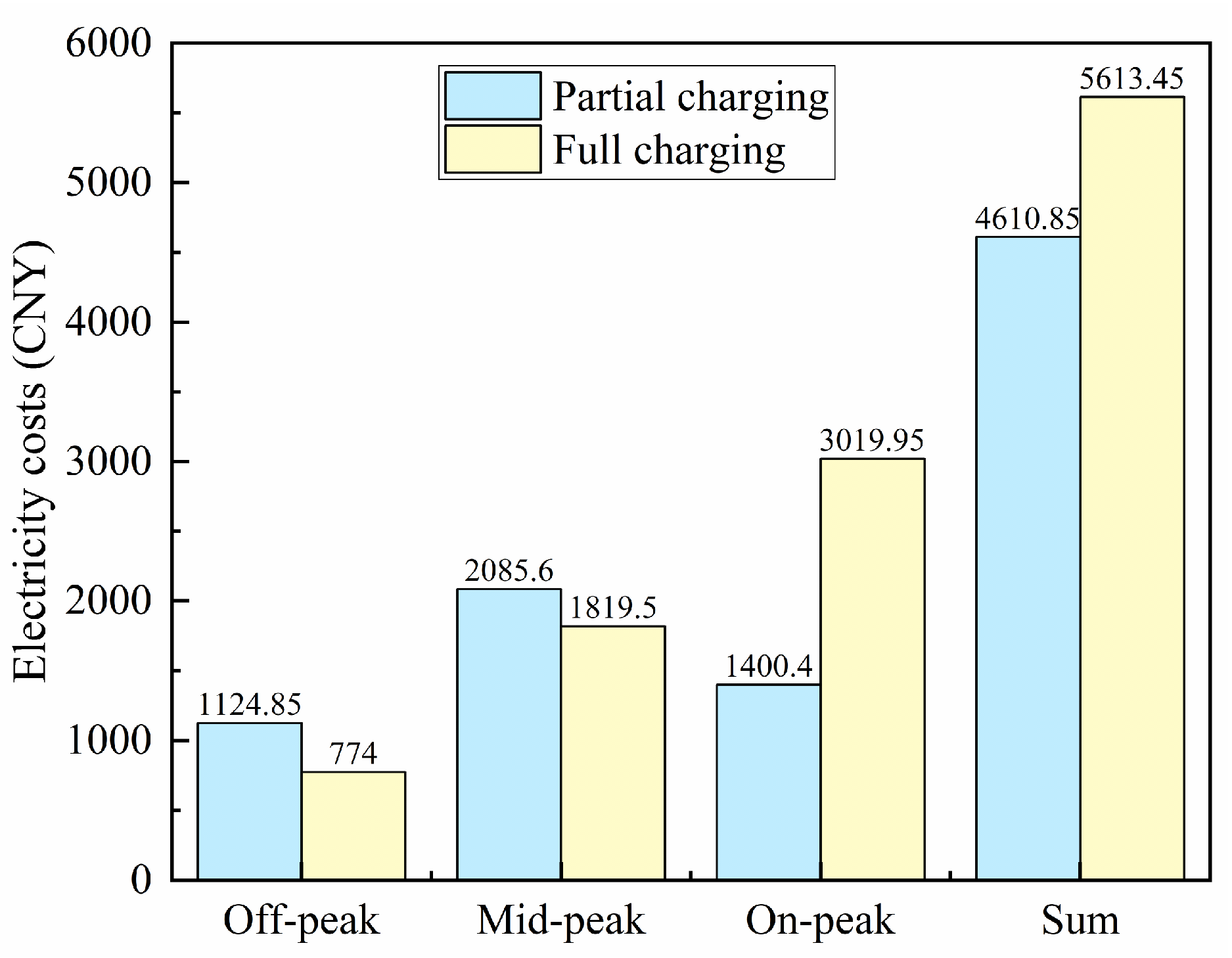
| Charging Strategy | Fleet Composition Costs | Purchase Costs of Chargers (CNY) | Electricity Costs (CNY) | Total Costs (CNY) |
|---|---|---|---|---|
| Partial Charging | 25,100.00 | 13,400.00 | 4610.85 | 43,110.85 |
| Full Charging | 25,700.00 | 13,400.00 | 5613.45 | 44,713.45 |
| Variation (%) | −2.33% | −0.00% | −17.33% | −3.58% |
Disclaimer/Publisher’s Note: The statements, opinions and data contained in all publications are solely those of the individual author(s) and contributor(s) and not of MDPI and/or the editor(s). MDPI and/or the editor(s) disclaim responsibility for any injury to people or property resulting from any ideas, methods, instructions or products referred to in the content. |
© 2025 by the authors. Licensee MDPI, Basel, Switzerland. This article is an open access article distributed under the terms and conditions of the Creative Commons Attribution (CC BY) license (https://creativecommons.org/licenses/by/4.0/).
Share and Cite
Zhang, M.; Mohamed, M.; Foda, A.; Guo, Y. Optimal Electric Bus Charging Scheduling with Multiple Vehicle and Charger Types Considering Compatibility. Sustainability 2025, 17, 3294. https://doi.org/10.3390/su17083294
Zhang M, Mohamed M, Foda A, Guo Y. Optimal Electric Bus Charging Scheduling with Multiple Vehicle and Charger Types Considering Compatibility. Sustainability. 2025; 17(8):3294. https://doi.org/10.3390/su17083294
Chicago/Turabian StyleZhang, Mingye, Moataz Mohamed, Ahmed Foda, and Yihua Guo. 2025. "Optimal Electric Bus Charging Scheduling with Multiple Vehicle and Charger Types Considering Compatibility" Sustainability 17, no. 8: 3294. https://doi.org/10.3390/su17083294
APA StyleZhang, M., Mohamed, M., Foda, A., & Guo, Y. (2025). Optimal Electric Bus Charging Scheduling with Multiple Vehicle and Charger Types Considering Compatibility. Sustainability, 17(8), 3294. https://doi.org/10.3390/su17083294