Article

Fuel Consumption Prediction for Full Flight Phases Toward Sustainable Aviation: A DMPSO-LSTM Model Using Quick Access Recorder (QAR) Data

1
College of Air Transportation, Shanghai University of Engineering Science, Shanghai 201620, China
2
Scania China Manufacturing Co., Ltd., Nantong 226500, China
3
Shanghai Shentong Metro Group Co., Ltd., Technical Center, Shanghai 201103, China
4
College of Civil Aviation, Nanjing University of Aeronautics and Astronautics, Nanjing 210016, China
5
SILC Business School, Shanghai University, Shanghai 201800, China
*
Authors to whom correspondence should be addressed.
Sustainability 2025, 17(8), 3358; https://doi.org/10.3390/su17083358
Submission received: 12 February 2025 / Revised: 31 March 2025 / Accepted: 4 April 2025 / Published: 9 April 2025

Abstract

:
Reducing emissions in the aviation industry remains a critical challenge for global low-carbon transition. Accurate fuel consumption prediction is essential to achieving emission reduction targets and advancing sustainable development in aviation. Aircraft fuel consumption is influenced by numerous complex factors during flight, resulting in significant nonlinear relationships between segment-specific variables and fuel usage. Traditional statistical and econometric models struggle to capture these relationships effectively. This article first focuses on the different characteristics of QAR data and uses the Adaptive Noise Ensemble Empirical Mode Decomposition (CEEMDAN) method to obtain more significant potential features of QAR data, solving the problems of mode aliasing and uneven mode gaps that may occur in traditional decomposition methods when processing non-stationary signals. Secondly, a dynamic multidimensional particle swarm optimization algorithm (DMPSO) was constructed using an adaptive adjustment dynamic change method of inertia weight and learning factor, which solved the problem of local extremum and low search accuracy in the solution space that PSO algorithm is prone to during the optimization process. Then, a DMPSO-LSTM aircraft fuel consumption model was established to achieve fuel consumption prediction for three flight segments: climb, cruise, and descent. The final proposed model was validated on real-world datasets, and the results showed that it outperformed other baseline models such as BP, RNN, PSO-LSTM, etc. Among the results, the climbing segment MAE index decreased by more than 40%, the RMSE index decreased by more than 38%, and the R2 index increased by more than 6%, respectively. The MAE index of the cruise segment decreased by more than 40%, the RMSE index decreased by more than 40%, and the R2 index increased by more than 5%, respectively. The MAE index of the descending segment decreased by more than 20%, the RMSE index decreased by more than 30%, and the R2 index increased by more than 5%, respectively. The improved prediction accuracy can be used to implement multi-criteria optimization in flight operations: (1) by quantifying weight–fuel relationships, it supports payload–fuel tradeoff decisions; (2) enhanced phase-specific predictions allow optimized climb/cruise profile selections, balancing time and fuel use; and (3) precise consumption estimates facilitate optimal fuel-loading decisions, minimizing safety margins. The high-precision fuel consumption prediction framework proposed in this study provides actionable insights for airlines to optimize flight operations and design low-carbon route strategies, thereby accelerating the aviation industry’s transition toward net-zero emissions.

1. Introduction

With the rapid development of the global economy and the increasing demand for civil aviation transportation, the pollution caused by aircraft fuel emissions is becoming increasingly serious. The emissions caused by aircraft fuel combustion are the largest source of carbon emissions in the aviation industry. According to the International Energy Agency (IEA), the carbon emissions from the aviation industry account for 12% of the global transportation sector’s carbon emissions in 2022, with an average annual growth rate of 3.5% [1]. The international community increasingly prioritizes energy conservation and emission reduction in civil aviation, with the promotion of green and sustainable development emerging as a global consensus [2]. The International Civil Aviation Organization (ICAO) passed the “2050 Net Zero Carbon Emissions” resolution in 2022, requiring a minimum of 2.5%/year increase in segment level fuel efficiency through technological innovation and operational optimization [3]. In this context, developing accurate fuel consumption prediction models is crucial for minimizing the gap between actual and theoretical fuel usage, enhancing fuel efficiency through technological innovation, and ultimately reducing carbon emissions—a key pathway toward sustainable aviation [4,5].
Early prediction methods involved calculating aircraft fuel consumption values based on aircraft performance manuals or energy models, which typically included models such as fuel consumption rate, thrust, drag/power ratio, and other parameters closely related to aircraft performance, aerodynamic characteristics, and flight path [6,7,8]. These parameters come from the performance manual of the aircraft manufacturer and need to be checked with a table. The accuracy is poor and the operation steps are cumbersome. They are not suitable for estimating the fuel consumption of the entire flight trajectory of the aircraft. Therefore, the European Organization for the Safety of Air Navigation (Eurocontrol) has developed the Aircraft Key Performance Database [9,10] and the Base of Aircraft Data (BADA). The BADA performance database provides various theoretical model specifications and related specific performance parameter datasets. It can realistically reproduce the aircraft’s motion trajectory throughout the entire flight phase based on existing aircraft performance reference data and then calculate the aircraft’s fuel consumption. Kaiser [11] and Dalmau [12] established a fuel consumption model based on the BADA database to avoid the tedious process of consulting static tables. Burzlaff [13] and Pagoni [4] developed a fuel consumption model using the BADA database to calculate the fuel consumption of an aircraft during flight. However, due to the lack of consideration of meteorological parameters, the accuracy of the aircraft fuel consumption model based on the BADA database is often low. To further enhance the practicality of prediction methods, researchers use statistical and mathematical methods to establish the aircraft fuel consumption model. Yutko [14] evaluated typical aircraft operations in order to develop evaluation hypotheses for task-based and instantaneous indicators. Jensen [15] conducted flight by flight analysis using over 200,000 historical operations conducted in 2012, considering the actual wind and temperature experienced by flights, and established an efficiency benefit pool to achieve full system cruise altitude optimization for domestic operations in the United States. However, due to the numerous and complex factors that affect aircraft fuel consumption during flight, there is a significant nonlinear relationship between the influencing factors of each flight segment and aircraft fuel consumption, which is difficult to explain using traditional statistical and econometric models.
This paper aims to dynamically adjust aircraft fuel transportation redundancy by establishing a predictive model to balance economy and safety. In order to build an accurate aircraft fuel consumption prediction model, effective data mining and analysis of performance parameters related to aircraft fuel consumption must be carried out to obtain more accurate aircraft fuel consumption prediction performance parameters. The neural network model, with its unique advantages of distributed storage and parallel processing, can approximate aircraft fuel consumption data with nonlinear performance relationships [16]. Therefore, this paper aims to explore the characteristics of QAR data for climb, cruise, and descent segments, using the CEEMDAN method to decompose aircraft fuel consumption data, fully exploring the changing characteristics of time series, and obtaining more detailed corresponding modal subsequences to provide good feature data for prediction models. A dynamic multidimensional particle swarm optimization algorithm (DMPSO) was developed to address the difficulty of parameter optimization in LSTM network models. The dynamic formula of inertia weight and learning factor was used to construct a DMPSO LSTM full range fuel consumption prediction model, which solves the problem of the particle swarm algorithm easily becoming stuck in local optima and low search accuracy in the solution space optimization process.
The structure of this article is as follows: Section 2 introduces the relevant research on machine learning-based fuel consumption prediction and estimation. Section 3 provides a detailed introduction to the fuel consumption prediction method based on the DMPSO-LSTM model. Section 4 introduces the application and result analysis of the proposed method on a certain airline’s A320 aircraft model. Section 5 provides a summary and future work.

2. Literature Review

2.1. Fuel Consumption Prediction

QAR (Quick Access Recorder) is a flight data recording system carried on aircraft, used for real-time acquisition, storage, and transmission of high-frequency flight operating parameters. Its recording range covers aircraft performance parameters (such as airspeed, altitude, attitude), engine status (such as fuel flow, speed, exhaust temperature), environmental conditions (such as temperature, wind speed), and control commands (such as flaps, throttle position), with a sampling frequency typically ranging from 1 to 4 times per second. QAR data are not only the core basis for aviation safety monitoring and accident investigation but also provide high-precision multidimensional data sources for flight performance analysis, fuel efficiency optimization, and prediction model construction. In the field of fuel consumption prediction, QAR data can effectively support data-driven fuel consumption modeling and abnormal pattern recognition by capturing dynamic parameters of the entire flight phase (such as climb rate, cruise Mach number, descent profile), combined with engine operating conditions and environmental variables [17,18]. QAR (Quick Access Recorder) data have become the core data source for aircraft fuel consumption prediction research due to its high-resolution and multidimensional flight parameter acquisition capabilities. In recent years, researchers have proposed various innovative methods by combining statistical modeling, machine learning, and flight performance theory.
Researchers construct a highly interpretable and computationally efficient prediction framework by mining physical correlations in QAR parameters and combining statistical learning techniques. Wang et al. [19]. proposed a hybrid model based on multiple linear regression and principal component analysis (PCA), which utilizes flight phase parameters (such as climb rate and cruise Mach number) and engine performance indicators (such as fuel flow rate and N1 speed) from QAR data to construct fuel consumption prediction equations for flight segments. Research has shown that the 10 key QAR parameters selected through PCA dimensionality reduction can explain 92% of the fuel consumption variance, but this method lacks adaptability to non-steady state flight conditions such as frequent speed regulation in turbulence. To enhance predictive robustness in complex scenarios, Smith and Jones [20] developed a Bayesian Hierarchical Model (BHM) that combines QAR data with aircraft performance benchmarks such as the BADA model. By quantifying the uncertainty of engine performance degradation and environmental wind speed through prior distribution, this model achieved an average absolute percentage error mean absolute percentage error (MAPE) of 3.8% in cross fleet prediction, which is 1.5% lower than traditional regression methods. This achievement highlights the advantages of mathematical statistical methods in integrating prior knowledge of physics with data uncertainty. In addition, García et al. [21] explored a generalized additive model (GAM) driven by QAR data, which fitted the correlation characteristics among flight altitude, airspeed, and fuel consumption through a nonlinear smoothing function. Its research confirms that segmented modeling based on QAR data statistical features (such as distinguishing between climb and cruise phases) can further reduce prediction errors by 12%, but it relies on high-precision flight phase automatic recognition algorithms for support. The International Air Transport Association (IATA) has evaluated the applicability of mathematical statistical methods in QAR data analysis and identified two major challenges that need to be addressed in current research: Firstly, the high dimensionality and multicollinearity of QAR parameters pose a risk of overfitting in traditional regression models. The second challenge is how to effectively identify significant operational variables that affect fuel consumption through statistical hypothesis testing (such as t-test, ANOVA), providing a basis for airlines to formulate fuel-saving strategies [22].
The current research has significantly improved prediction accuracy through physical statistical hybrid modeling and staged parameter optimization, but further efforts are needed to balance the model’s generalization ability and real-time performance, while strengthening the standardization process of QAR data quality control and feature engineering. The prediction of aircraft fuel consumption is a very complex multivariate time series fitting problem, and machine learning neural networks are very suitable for nonlinear data fitting budgets. Therefore, using neural network models to predict aircraft fuel consumption has become a research hotspot. This type of method significantly improves the prediction accuracy under complex operating conditions by capturing the nonlinear relationships and spatiotemporal dependencies between flight parameters. Zhang et al. [23] first proposed a framework combining Long Short-Term Memory (LSTM) and Convolutional Neural Network (CNN), which utilizes time series parameters (such as fuel flow rate, airspeed, altitude) and engine state sequences from QAR data to achieve a segment level fuel consumption prediction error of less than 1.5%. This model extracts local features (such as instantaneous fuel consumption fluctuations during the climb phase) through CNN and combines LSTM to model cross stage dependencies, but its computational complexity limits its real-time deployment capability. To optimize the efficiency of feature extraction, Liu et al. [24] designed an attention-based Transformer architecture that embeds QAR parameters (such as N1 RPM, ambient temperature) and flight phase labels (climb, cruise, descent) into multidimensional vectors. The experiment shows that this model reduces the error by 18% compared to traditional LSTM in long haul route prediction and has stronger robustness to data loss. However, the problem of insufficient interpretability has not been solved, making it difficult to quantify the contribution of a single parameter to fuel consumption. In response to the demand for multi-source data fusion, Chen et al. [25] developed a graph neural network (GNN) model that integrates QAR data, radar trajectories, and meteorological grid information to construct a fuel consumption map for the entire flight cycle. This model represents the dynamic fuel consumption correlation between waypoints through graph nodes and improves prediction accuracy by 23% in complex airspace environments such as detours and waiting routes. To further optimize feature engineering, Liu and Wang [26] developed an anomaly detection framework based on QAR data, which identifies fuel efficiency losses caused by non-standard operations (such as non-economic climb rates) by analyzing the synergistic relationship among engine speed (N1), exhaust temperature (EGT), and fuel flow rate. Its research confirms that manipulation features in QAR data, such as flap angle and throttle lever position, can serve as key inputs for predictive models to distinguish the impact of pilot operating preferences on fuel consumption. However, this method has limited modeling capabilities for route structures, such as path deviations caused by air traffic control instructions. In response to the prediction needs in complex airspace environments, Chen et al. [27] proposed a spatiotemporal feature fusion model that combines QAR data with radar trajectories and air traffic control instructions (such as altitude changes and waiting routes) and uses graph neural networks (GNNs) to model the fuel consumption dependency between waypoints. Experiments have shown that this model improves prediction accuracy by more than 15% compared to traditional regression methods in flights with frequent speed adjustments and path extensions. This achievement highlights the potential of collaborative modeling between QAR data and external operating environments but also points out that the current research still needs to improve the balance between real-time data and computational efficiency. Meanwhile, in recent years, researchers have further focused on the collaborative mechanism between fuel consumption prediction and sustainable aviation. Schäfer et al. [28] quantified the reduction effect of route optimization on carbon emission intensity by integrating QAR data with airspace structure parameters. They demonstrated that for every 1% decrease in fuel consumption prediction error during the climb phase, the carbon footprint of the entire flight segment can be reduced by 0.6%. Zhang et al. [29] developed a multi-objective optimization framework based on LSTM, which generates carbon budget schemes that meet CORSIA standards while predicting fuel consumption, but the cross stage dynamic coupling problem has not been solved. In addition, the International Air Transport Association (IATA) has pointed out that existing predictive models have insufficient interpretability in supporting the preparation of ESG (Environmental, Social, and Governance) reports by airlines, and there is an urgent need for a hybrid modeling method that integrates physical mechanisms and data-driven approaches [30]. The “Fuel Efficiency Benchmark 2023” released by Airbus shows that the A350-1000 model reduces additional fuel carrying capacity by 7% to 12% through dynamic prediction and reduces CO2 emissions by 3200 tons annually [31].

2.2. Knowledge Gap

Traditional empirical models, such as the BADA database and energy-based equations, rely on aerodynamic and thermodynamic principles to estimate fuel consumption. While these models provide interpretable results, they often lack adaptability to real-world operational variations (e.g., turbulence, engine degradation). For instance, the BADA model assumes ideal flight conditions and neglects transient effects during phase transitions, leading to average prediction errors of 8–12% in real-world datasets [4,12]. In contrast, data-driven approaches leverage high-resolution QAR data to capture nonlinear relationships between operational variables (e.g., vertical acceleration, wind speed) and fuel consumption, enabling higher accuracy under dynamic conditions. According to current research, there are still significant knowledge gaps at the following theoretical levels:
(1) Efficient decomposition and feature preservation of non-stationary QAR signals. Existing research generally adopts traditional signal decomposition methods (such as EMD and wavelet transform) to process QAR time series data but has not effectively solved the problems of mode aliasing and non-uniform gaps. This leads to the inability of the decomposed subsequence to accurately characterize the dynamic characteristics of the flight phase (such as instantaneous fuel consumption fluctuations in turbulence), limiting the adaptability of the model to complex operating conditions.
(2) Lightweight characterization and physical interpretability of high-dimensional QAR data. Existing methods such as PCA and linear regression are prone to losing the physical correlation of QAR parameters during dimensionality reduction and have not solved the coupling problem between high-dimensional features and nonlinear fuel consumption relationships. For example, although PCA reduces dimensionality, it cannot preserve the nonlinear mapping between aerodynamic efficiency parameters (such as the lift to drag ratio) and fuel consumption.
(3) Adaptive modeling and collaborative optimization during the dynamic flight phase. The current research focuses on the independent modeling of the climb, cruise, and descent stages, neglecting the dynamic coupling effects across stages (such as the impact of the end of climb on the initial fuel consumption during cruise). In addition, traditional PSO algorithms are prone to becoming stuck in local optima when optimizing LSTM hyperparameters, and do not consider the impact of flight phase differences on the parameter search space.

3. Methodology

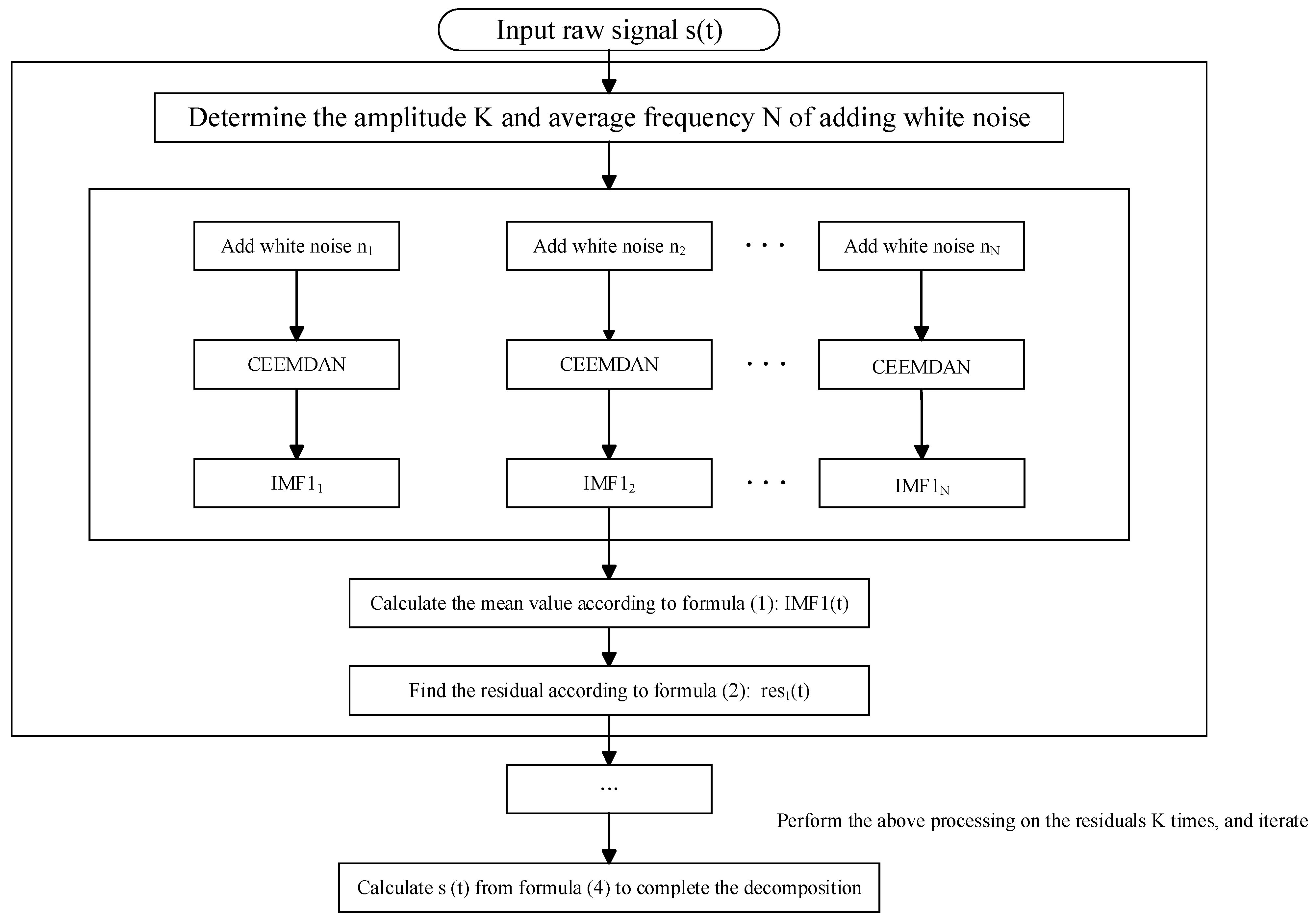
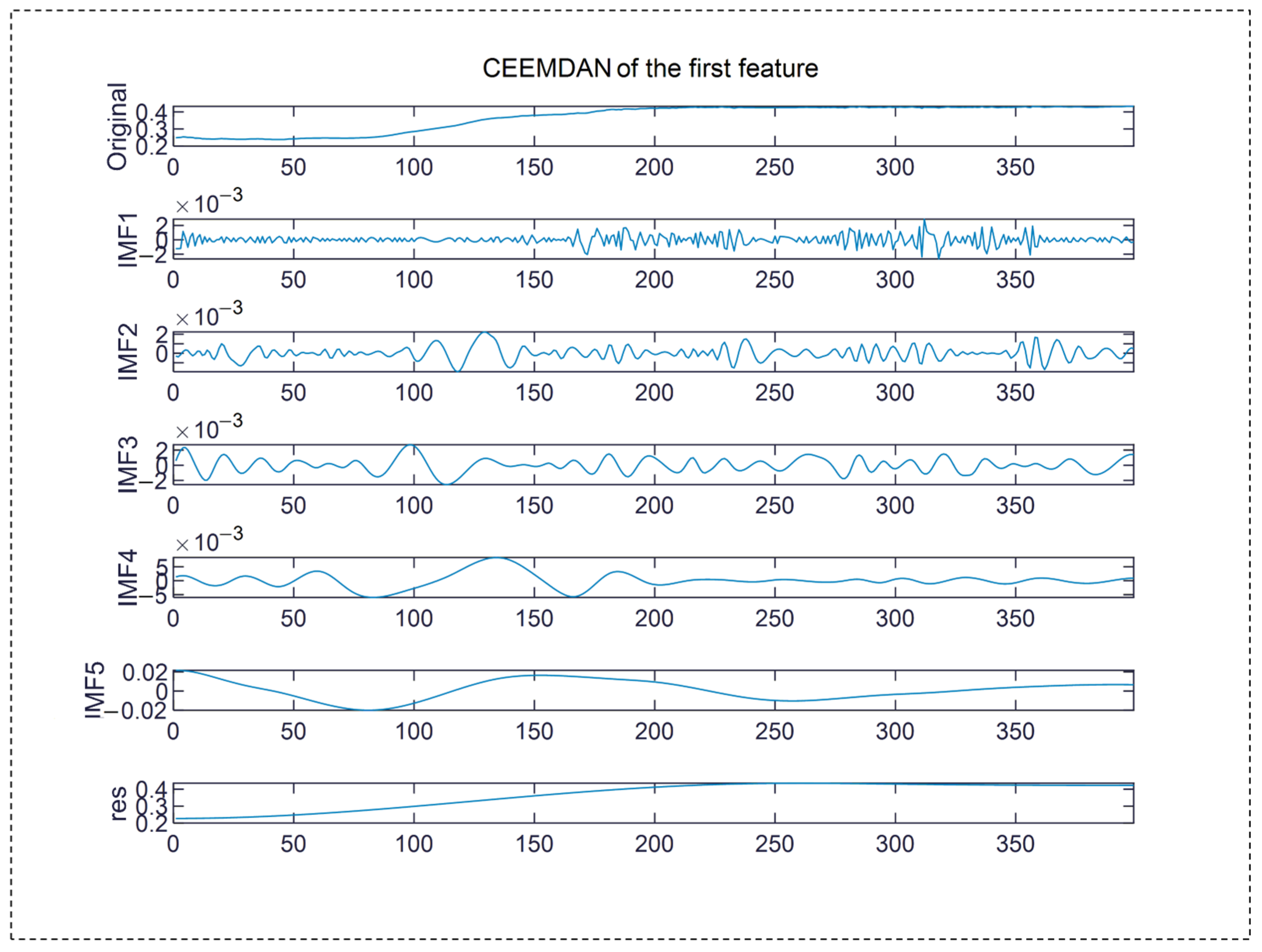
3.1. Decomposition of Fuel Consumption Impact Characteristics Based on CEEMDAN

QAR data have non-stationary and nonlinear characteristics, and the characteristics of data in different time periods are different. In response to this situation, the Complete Ensemble Empirical Mode Decomposition with Adaptive Noise (CEEMDAN) method is first used to decompose the aircraft fuel consumption data, fully utilizing the changing characteristics of the time series to obtain a more detailed subset of relevant modes, providing good feature data for the prediction model.
Complementary Ensemble Empirical Mode Decomposition (CEEMDAN) with Adaptive Noise is a further improved decomposition method based on Empirical Mode Decomposition (EMD) and Ensemble Empirical Mode Decomposition (EEMD) [32,33]. The CEEMDAN method first determines the final IMF component of the original signal, then adds white noise and iterates. The decomposition process is as follows:
(1) Preprocess the signal to avoid extreme values or monotonic trends.
(2) Construct an adaptive noise sequence and add it to the original signal to generate multiple sets of random experimental signals.
(3) Perform CEEMDAN on each experimental signal to obtain a set of IMFs.
(4) Combine and weight each group of IMFs to generate a set of total IMFs.
(5) Perform CEEMDAN on the total IMF to obtain a new set of IMFs.
(6) Check whether the newly generated IMF meets the convergence condition. If not, return to step (2) to adjust the adaptive noise.
(7) After satisfying the convergence condition, iterate repeatedly according to steps 3–6 until the number of IMFs obtained no longer increase.
In the CEEMDAN process, different IMFs have different fluctuation characteristics, resulting in the original data having different fluctuation characteristics at different time intervals. CEEMDAN captures the instability, randomness, and variability of the original time series data through intrinsic mode functions (IMFs), effectively highlighting localized features across different temporal scales. The flowchart of the CEEMDAN feature decomposition algorithm is shown in Figure 1.
The specific decomposition process is as follows:
(1) If the original data sequence of factors affecting aircraft fuel consumption for each flight segment (represented by s(t)) adds noise with a mean of 0 (represented by φ j ( t ) ) before decomposition, then s(t)+ α 0 φ j (t) is the new original decomposition sequence. On the other hand, parameter α 0 is used to ensure that the signal-to-noise ratio of the added noise to the original signal remains within an acceptable range and can be adjusted accordingly. The standard deviation of φ j ( t ) is kε, k is the coefficient of the noise fluctuation amplitude value, and ε is the standard deviation of the sequence.
(2) Perform CEEMDAN on the s(t) + α 0 φ j (t) sequence.
(3) Repeat steps (1) and (2) N times, adding different noise sequences φ j (t) in each execution, where the first modal component is the average of the components in N executions, calculated as shown in Equation (1), and the remaining r e s 1 t are the differences between the initial data and the modal components, calculated as shown in Equation (2).
I M F 1 t ~ = 1 N j = 1 N I M F 1 j ( t )
  r e s 1 t = s t I M F 1 t ~ ~
(4) Continuing to introduce white noise and residuals to eliminate errors caused by adding noise, the new signal to be decomposed is r e s 1 t + α 1 E M D 1 ( φ j ( t ) ) . The calculation formula for the second modal component is shown in Equation (3).
I M F 2 t ~ = 1 N j = 1 N E M D ( r e s 1 t + α 1 E M D 1 ( φ j ( t ) ) )
(5) Repeat step (4) until the residual r e s i t satisfies the termination condition, obtaining M specific modal components and the final residual r e s t . The calculation method for the final initial signal sequence is shown in Equation (4).
s t = i = 1 M     I M F 1 t ~ +   r e s t

3.2. Dimension Reduction in Aircraft Fuel Consumption Impact Characteristics Based on KPCA

The data sequence obtained through CEEMDAN highlights the fluctuation characteristics of the original data at different time scales, but the dimensionality of the input data variables also increases accordingly. To enhance computational efficiency and mitigate overfitting, the kernel principal component analysis (KPCA) algorithm is employed for dimensionality reduction in input variables, thereby improving the computational efficiency and accuracy of the model while retaining the effectiveness and representativeness of information. KPCA introduces the idea of kernel functions, which map data from low dimensions to high dimensions by performing inner product operations in space. Data extraction can be achieved without specifying a specific mapping function, and the introduction of kernel functions further reduces the computational complexity of the entire system. The implementation steps are as follows:
(1) For a given m n -dimensional original sample set X with a total of m samples, the covariance matrix is first calculated using the method shown in Equation (5).
C ¯ = 1 N i = 1 N ( X i ) ( X i ) T
Among them, ( X i ) is the nonlinear mapping function in the conversion process, and i = 1 N ( X i ) = 0 .
(2) According to the covariance matrix, calculate the corresponding decomposition eigenvalue V, and corresponding eigenvector V, as shown in Equations (6) and (7).
λ V = C ¯ V = 1 N i = 1 N ( X i ) T , V ( X i ) λ V
V = i = 1 N ( X i )
(3) By introducing the kernel function matrix into the nonlinear mapping function, p sets of kernel principal elements can be obtained, where the calculation method for the k-th principal element is shown in Equation (8).
t k = V k , ( x ) = i = 1 N α i k X i , ( x )     ( k = 1,2 , , p )
Gaussian radial basis functions are chosen as the kernel functions because they have fewer parameters and are semi-positively defined symmetric functions. The calculation method is shown in Equation (9).
k x , y = e | x y | 2 2 σ 2
(4) According to the set of main elements, statistical measures reflecting the degree of data model fitting and data trend can be obtained. The calculation method of the KPCA model statistical measures is shown in Equation (10).
T 2 = t 1 , , t p Λ 1 t 1 , , t p T
The stability of KPCA data is often evaluated using the T 2 statistic, which represents the distance between the sample data and the mean of the variable data in the high-dimensional KPCA space. This reflects the degree to which the aircraft fuel consumption data deviates from the stable operating state in terms of trend and amplitude. In the equation, t 1 , , t p is the principal component of the aircraft fuel consumption data extracted by KPCA, which can be calculated according to Equation (8). Λ 1 is the diagonal inverse matrix composed of the eigenvalues corresponding to each principal component.

3.3. Aircraft Fuel Consumption Prediction Model Based on Improved PSO-LSTM

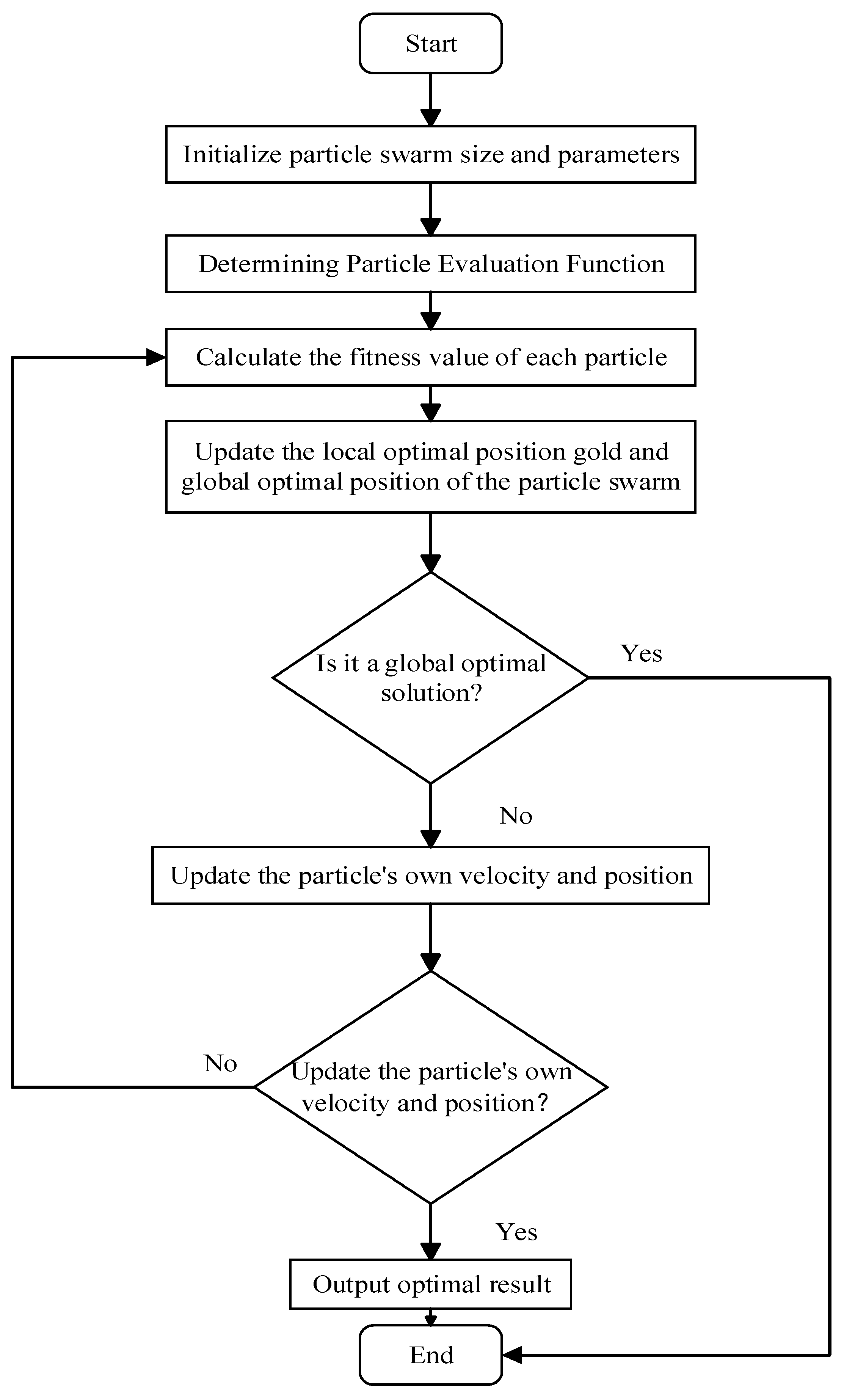
3.3.1. DMPSO Algorithm

Particle swarm optimization (PSO) [34] is a random parallel search algorithm that simulates the foraging behavior of birds and fish in nature. It consists of a set of particles, where one particle moves in the search space based on its best position ( p b e s t ) and the best position reached by any particle entering the particle swarm ( g b e s t ). All particles have velocities, positions, and corresponding fitness values that determine their direction of motion. The particles will follow the particle with the best historical fitness value and search for a solution in space until they work together in a group to find the optimal solution and corresponding fitness value for the problem to be optimized. The process of PSO is shown in Figure 2, and the specific steps are as follows.
(1) In the D-dimensional solution space, assuming the number of particles is m, the inertia weight is w, the acceleration constants are c 1 and c 2 , and the random numbers are r a n d 1 d and r a n d 2 d .
(2) Randomly initialize the initial position x and initial velocity v of each particle and evaluate the fitness value of each particle to obtain the current individual optimal position solution p b e s t and the global optimal position solution g b e s t .
(3) Update the particle position and velocity according to the following Formulas (11) and (12):
v i d = v i d + c 1 r a n d 1 d ( p b e s t i d x i d ) + c 2 r a n d 2 d ( g b e s t i d x i d )
x i d = x i d + v i d
Among them,   p b e s t i d and g b e s t i d respectively refer to the optimal position searched by the i-th particle and the entire particle swarm in d-dimensional space; x i d and v i d respectively refer to the position and velocity of the particle corresponding to the d-th variable.
(4) Calculate the fitness value of each particle’s function and update the individual optimal position solution p b e s t and global optimal position solution g b e s t of the particle.
(5) Continuously iterate until the specified termination condition is met, then stop searching and output the optimal result, otherwise return to step (3).
However, the main problem with traditional PSO algorithms is that they are prone to becoming stuck in local optima during the optimization process, which can lead to lower search accuracy. In order to accelerate convergence speed and avoid becoming stuck in local optima, this paper constructs a dynamic multidimensional particle swarm optimization algorithm (DMPSO). This algorithm utilizes a dynamically changing formula adaptively adjusted by inertia weights [34,35] and learning factors [36,37] to transform fixed parameters into nonlinear transformation parameters, in order to improve the accuracy and speed of convergence. The specific details are as follows.
(1) Adaptive optimization of inertia weight ω. The inertia weight not only determines the influence of the particle’s historical flight state on the current flight speed but also balances the global search ability of the particle swarm algorithm. In order to improve the optimization performance of particle swarm optimization algorithm, in the early optimization stage, the global search ability of each particle should be expanded as much as possible, while in the later optimization stage, it is more desirable to have higher fine search ability. This article introduces a nonlinear decreasing inertia weight adaptive adjustment method, which not only gradually reduces the weight value as the number of runs increases, thereby achieving the goal of transforming the particle swarm algorithm from early global search to later fine search mode, but also effectively overcomes the problem of poor local search ability in the later stage of linear decreasing weight. The improved calculation method is shown in Equation (13).
w = a a b t N
In the formula, a and b are the maximum and minimum values of the inertia weight, t is the current number of iterations, and N is the maximum number of iterations.
(2) Adaptive optimization learning factors c 1 and c 2 . The learning factor c 1 is the expression of particle self-awareness, used for the influence of self-awareness on flight trajectories, and c 2 is the expression of particle group consciousness, used for the influence of social cognition on flight trajectories. In the early stages of optimization, the focus must be on the individual’s self-awareness, while in the later stages, the focus must be on the individual’s cognitive ability to acquire social information. Therefore, in order to balance the influence of learning factors on flight trajectories, an optimization method was introduced where the learning factors adaptively change with inertia weights. The improved calculation formulas are shown in Equations (14) and (15), respectively.
c 1 = e 1 e 1 e 2 c o s ( w )  
c 2 =   f 1 + f 2 f 1   c o s ( w )    
In the formula, w is the inertia weight, e 1 and f 1 are the initial values of the learning factor, and e 2 and f 2 are the termination values for the learning factor.

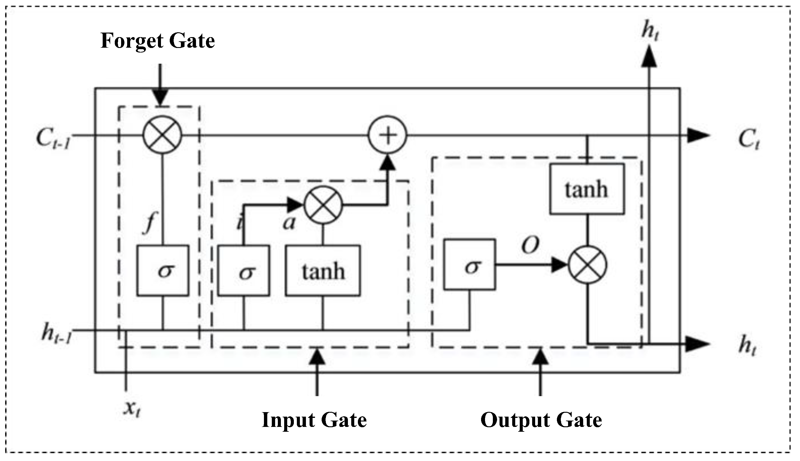
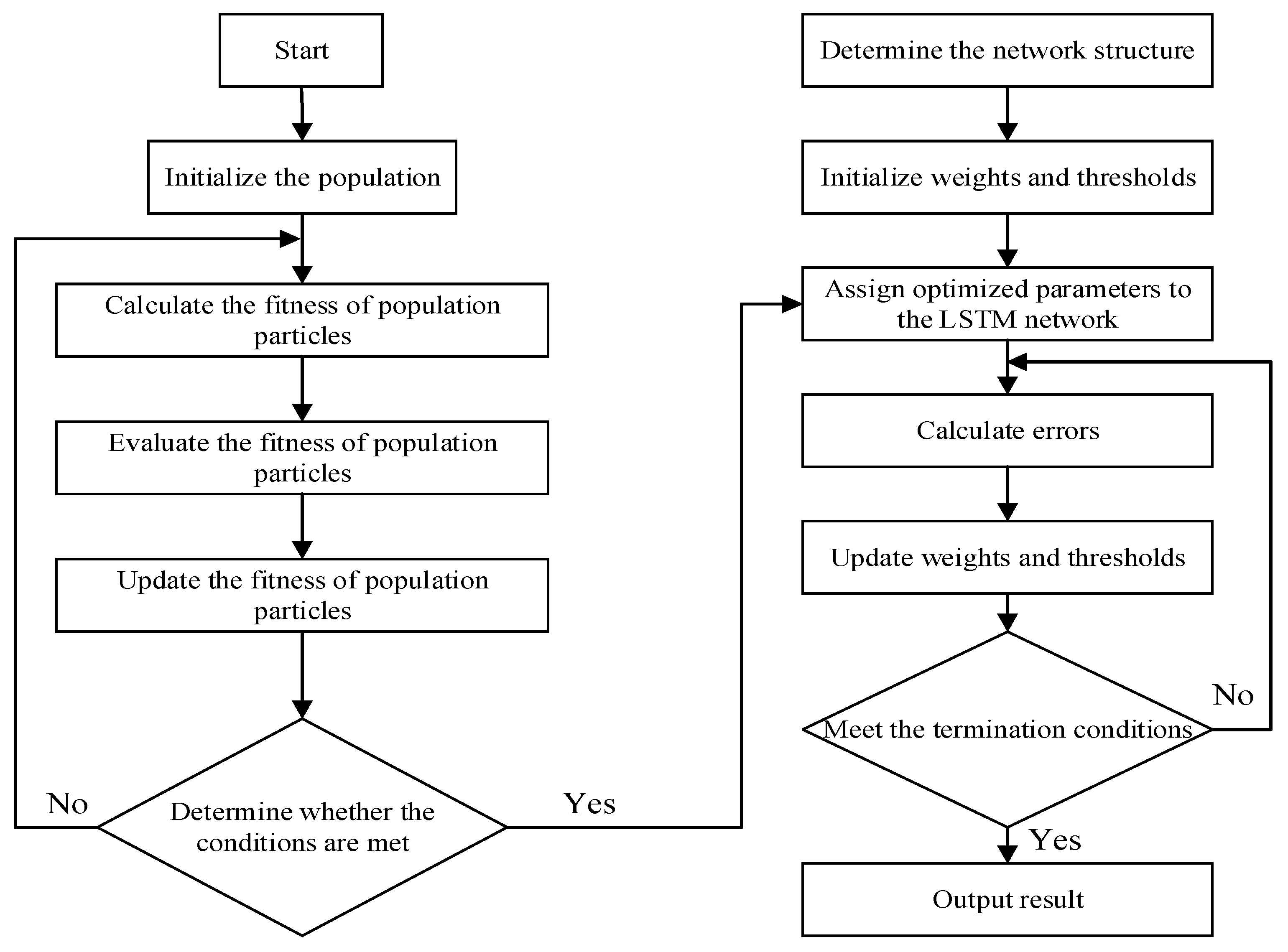
3.3.2. DMPSO-LSTM Model

Long Short-Term Memory Network (LSTM) is a special type of RNN with memory properties [38]. LSTM introduces a control input/output unit structure consisting of forget gates, input gates, and output gates. During information transmission, due to the unique internal structure of the storage unit, this structure can maintain a stable error flow, ensuring that the entire network does not cause gradient explosion or vanishing during training. It also has excellent memory performance and is very suitable for classifying, processing, and predicting time series data. The structure diagram of the LSTM network model is shown in Figure 3. Among them, f is the forget gate, i is the input gate, a is the output gate, Ct is the update process of the cell state, xt is the input at the current time point, ht is the hidden state at the current time point, ht-1 is the hidden state at the previous time point, and O is the output after function processing.
The values of parameters such as learning rate, step size, and iteration times in the LSTM model can affect the prediction results of the model. In order to avoid subjective factors in the parameter selection process and explore more reasonable and effective methods for predicting aircraft fuel consumption, a dynamic multidimensional particle swarm optimization algorithm (DMPSO) is proposed to optimize the learning parameters in the LSTM neural network, that is, to establish a DMPSO-LSTM model to predict the time series of aircraft fuel consumption.
The DMPSO-LSTM model takes the batch size, number of hidden layer units, time window size, and other related parameters of the LSTM model as optimization objects and uses an improved PSO algorithm to adjust and optimize its parameters. The flowchart for optimizing the LSTM model with DMPSO is shown in Figure 4.
The specific process is as follows:
(1) PSO algorithm parameter initialization encoding. Initialize particle swarm parameters such as inertia weights, population size, iteration times, learning factors, and parameter solving intervals based on the LSTM parameters to be optimized.
(2) Determine the optimization parameters and range. Initialize the position x and velocity v of the particle swarm with the batch size, number of hidden layer units, and time window size of the LSTM model as the parameters to be solved and ensure that x and v are within the solution interval of the parameters.
(3) Calculate and evaluate the fitness function. Select the loss function of LSTM on the training set as the individual fitness function of the algorithm and initialize the global optimal particle position solution g b e s t and the local optimal particle position solution p b e s t based on the principle of minimizing fitness values.
(4) Update the fitness of the particle population. Calculate the weights and learning factors of the particle swarm based on Equations (13)–(15), and update p b e s t and g b e s t in real-time.
(5) Determine termination conditions. If satisfied, terminate the iteration and return the optimal parameter value, otherwise return to step (3).
(6) Output the result. Substitute the parameters into the LSTM neural network for training and output the prediction results through the test dataset.
The DMPSO-LSTM model structure consists of an input layer, two LSTM layers, and an output layer. The optimal parameter time window size of the adaptive particle swarm model is set to 10, the learning factors c 1 and c 2 are 1.5, the batch size is 60, the number of hidden layer units in the first layer is 12, the number of hidden layer units in the second layer is 22, the learning rate is set to 0.001, and the particle swarm population size is set to 30. The maximum iteration number is 500, and the velocity inertia weight w is 0.8. The Adam algorithm is used to optimize the model training process, and the loss function uses mean square error. The initial parameter settings for the DMPSO LSTM aircraft fuel consumption prediction model is shown in Table 1.

4. Case Study

The QAR data used in this article are selected from the QAR data of a reference airline’s A320 aircraft model as the experimental source, including 27,015 flight records. The QAR system captures a large amount of flight parameters and operational data from onboard systems, including time, takeoff airport, landing airport, aircraft type, takeoff runway, altitude, speed, heading, fuel consumption, and other data. Table 2 shows some sample data.
The influencing factors for the final selection of the climb, cruise, and descent segments are shown in Table 3. The overall framework of the DMPSO-LSTM aircraft fuel consumption prediction model is shown in Figure 5. The overall process steps are as follows:
(1) Perform CEEMDAN on the fuel consumption influencing factors of each flight segment after data preprocessing to reduce its volatility.
(2) Use the kernel principal component analysis (KPCA) method to reduce the dimensionality of decomposed data with fewer input parameter dimensions.
(3) Use the DMPSO algorithm to optimize the optimal values of the LSTM network parameters and reduce the random errors caused by the manually set LSTM network parameters.
(4) The LSTM network optimized using the DMPSO algorithm is used to make preliminary predictions for the decomposed reconstructed sequence and residual sequence, respectively.

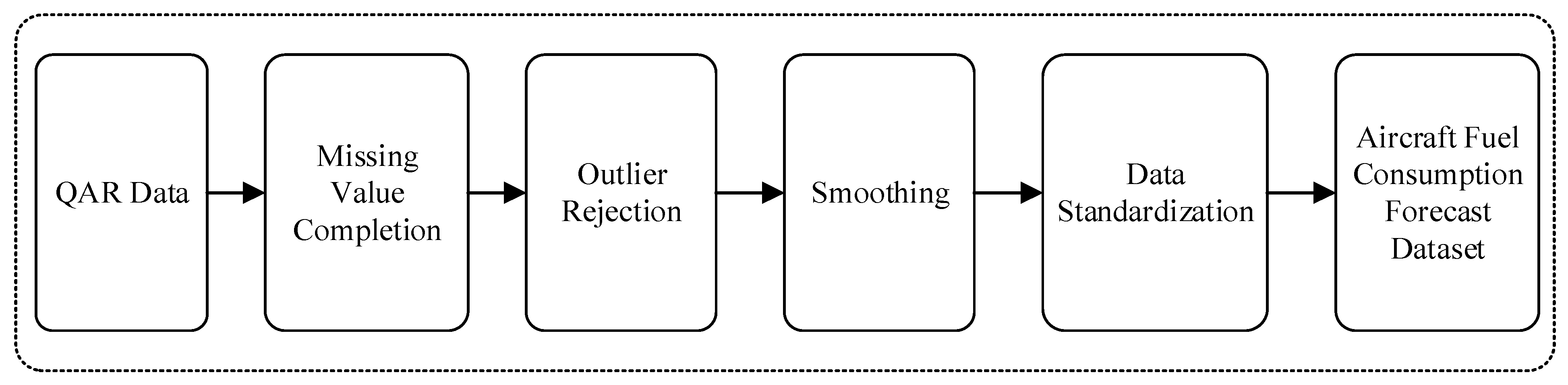
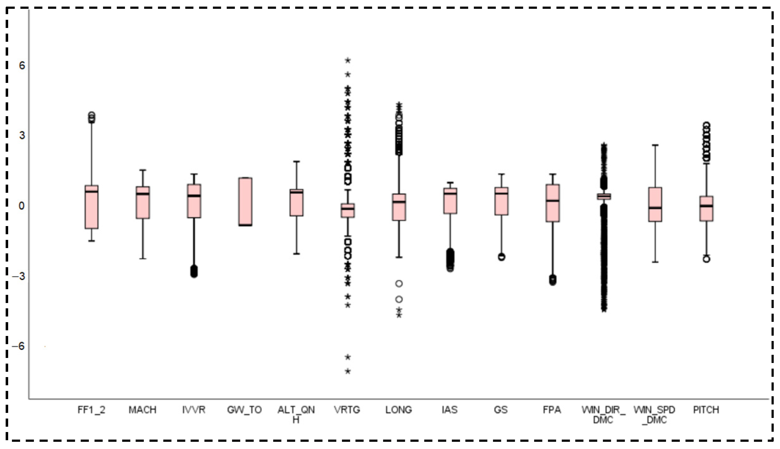
4.1. Data Preprocessing

This article will use methods such as missing value completion, outlier removal, moving average smoothing, and data normalization to preprocess QAR data, in order to construct a dataset for aircraft fuel consumption prediction based on neural networks. The dataset generation process is shown in Figure 6.
This paper uses the mean interpolation method to complete missing values. The mean interpolation method interpolates data based on the average value of the sample data or the average value of multiple samples. The calculation method is shown in Equation (16).
y ¯ = i = 1 n β i y i n i
Among them, βi is a descriptive symbol indicating whether to answer, βi = 1 represents “yes”, βi = 0 means “no”, and ni is a number.
Due to sensor malfunctions or errors, abnormal data collection and transmission, as well as flight operations and operating conditions, outliers are prone to occur in the QAR dataset. Figure 7 is a box plot of the selected QAR parameter data.
From Figure 7, it can be seen that in the QAR data of the selected parameters, there are no outliers in the Mach number (MACH), aircraft weight (GW_TO), and barometric altitude (ALT_QNH) parameter columns. However, there are outliers in the remaining total fuel flow rate (FF1_2), vertical velocity (IVVR), vertical acceleration (VRTG), longitudinal acceleration (LONG), airspeed (IAS), ground speed (GS), tilt angle (FPA), wind speed (WIN_SPD_DMC), wind direction (WIN_DIR_DMC), and pitch angle (PITCH). This paper uses box plot analysis to remove outliers. The principle of removing outliers in box plots is based on the statistical method of interquartile range (IQR). The standard for removing outliers from box plots is to use the quartiles and interquartile range of the box plot to experimentally test the data. If the monitored data appears outside the box plot, it is abnormal data and needs to be removed. Circles represent ordinary outliers and asterisks indicate extreme outliers or multiple overlapping outliers.
This paper uses the moving average method to process noisy data. It is a method of smoothing the window by moving the average over the data to denoise the data. The algorithm not only has the advantage of low complexity but also can remove short-term fluctuations in the time series, making the data smoother and eliminating differences between various sample data of aircraft fuel consumption. Figure 8 shows the implementation results of the moving average method for smoothing different windows. From Figure 8, it can be seen that the setting of different windows in the moving average method has a significant impact on the effectiveness of data smoothing. When the window size is set to 3, the smoothed QAR data almost retain the local variation characteristics of the original aircraft fuel consumption data. As the window size increases, the smoothed QAR data curve becomes smoother but also lags more. When the window size is set to 9, the smoothed QAR data are too smooth to present the changes between adjacent time series. To preserve as much local variation as possible in the original aircraft fuel consumption QAR data, remove unnecessary noise, and obtain relatively smooth aircraft fuel consumption data, this section chooses to set the window size for smoothing processing to 5 in order to prepare for further analysis of aircraft fuel consumption characteristics and model construction.
Due to the different dimensions and units of QAR data parameters, in order to eliminate the influence of different parameter data ranges on prediction results, it is necessary to use the same dimensions or standardized data for the data before establishing the model. This article uses normalization to process the data, converting the processed data parameters into dimensionless data between [0, 1], thereby eliminating errors and improving prediction accuracy. The conversion method is shown in Equation (17).
X t n ˙ = X t n X t m i n X t m a x X t m i n
where X t n ˙ is the normalized value of the n-th value in the t-th parameter, X t n is the value before normalization of the n-th value in the t-th parameter, X t m a x is the maximum value in the t-th parameter, and X t m i n is the minimum value in the t-th parameter. The partial data after normalization are shown in Table 4, where the unit of fuel volume is kg.

4.2. Decomposition and Dimensionality Reduction in Factors Affecting Aircraft Fuel Consumption

4.2.1. Decomposition of Factors Influencing Aircraft Fuel Consumption Characteristics

The CEEMDAN algorithm is used to decompose the data sequence of factors affecting aircraft fuel consumption, and 500 sets of noise pairs are added to the decomposition algorithm with a noise amplitude set to 0.2. The input data of this algorithm is the data sequence of factors affecting aircraft fuel consumption in each flight segment, and the output is the IMF component and residual component (res). According to the adaptive decomposition performance of the algorithm, the Mach number data sequence was decomposed into seven sets of IMF components of different scales and one set of residual components by CEEMDAN. The decomposition results are shown in Figure 9.
The number of IMF components and remaining components obtained by decomposing the factors affecting aircraft fuel consumption during the climb, cruise, and descent segments using CEEMDAN is shown in Table 5, Table 6 and Table 7.

4.2.2. Dimensionality Reduction in Aircraft Fuel Consumption Impact Characteristics

Use KPCA algorithm to perform dimensionality reduction on the data sequence obtained through CEEMDAN, with kernel function parameters set to 10, total input dimension set to 2, and cumulative contribution rate set to principal components greater than 95%. The individual feature contribution rates of the climb segment, cruise segment, and descent segment after KPCA dimensionality reduction are shown in Figure 10, Figure 11 and Figure 12.
From the above experimental results, it can be seen that after KPCA dimensionality reduction, the contribution rates of the principal component numbers of the decomposed feature sequence are sorted from high to low, and the principal component numbers with relatively high contribution rates are selected based on a cumulative contribution rate of 98%. As a result, the factors affecting aircraft fuel consumption during the climb segment decreased from 71 dimensions to 10 dimensions, the factors affecting aircraft fuel consumption during the cruise segment decreased from 71 dimensions to 9 dimensions, and the factors affecting aircraft fuel consumption during the descent segment decreased from 60 dimensions to 9 dimensions.

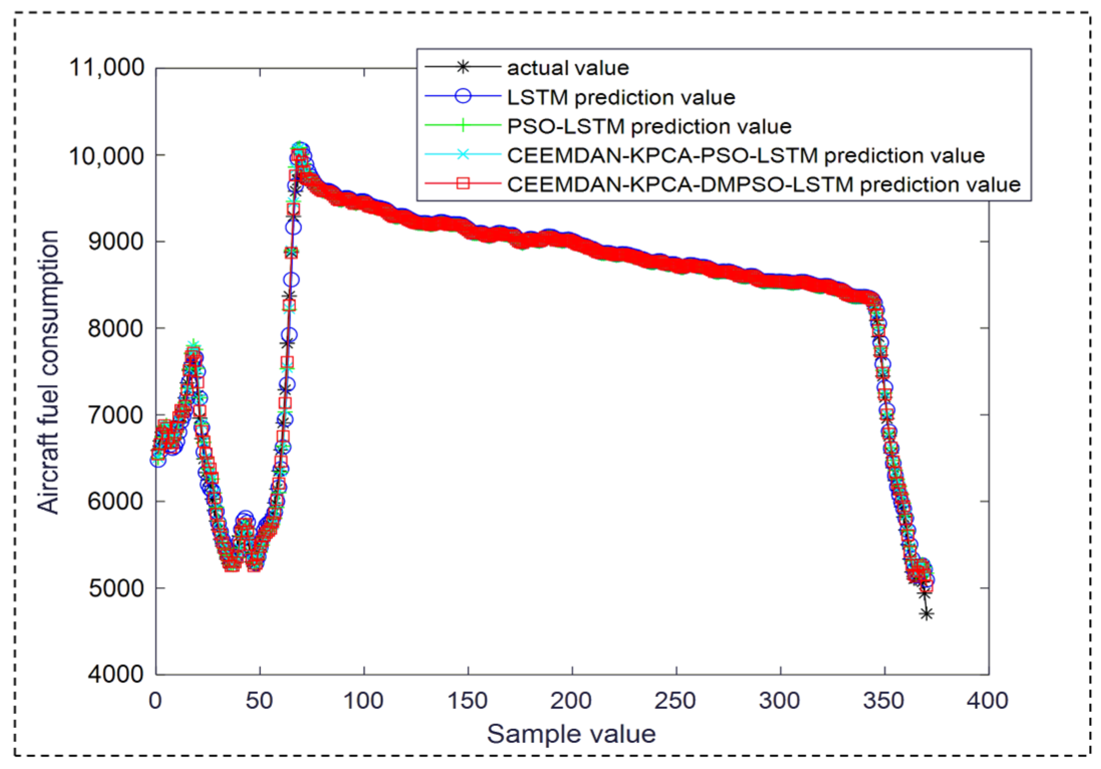
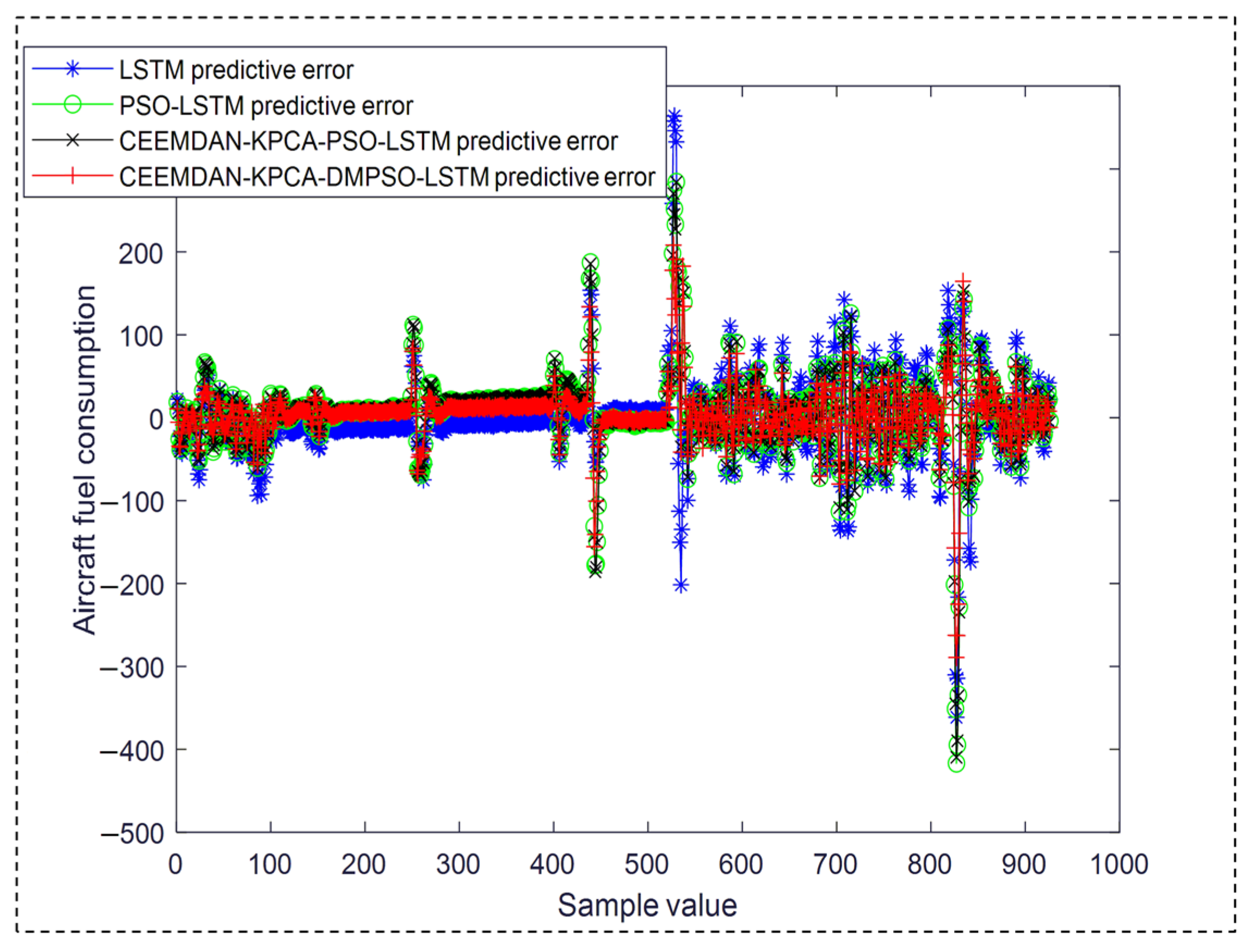
4.3. Experimental Results

To verify the effectiveness of the proposed model, this paper compared the prediction results of four models: LSTM, CEEMDAN-PSO-LSTM, CEEMDAN-KPCA-PSO-LSTM, and CEEMDAN-KPCA-DPSO-LSTM. The comparison of aircraft fuel consumption prediction results for the climb, cruise, and descent segments is shown in Figure 13, Figure 14 and Figure 15, and the corresponding prediction errors for each segment are shown in Figure 16, Figure 17 and Figure 18. It can be seen from the figure that the CEEMDAN-KPCA-DMPSO-LSTM aircraft fuel consumption prediction model proposed in this paper has higher prediction accuracy than the single model that has not been optimized, whether in the climb leg, cruise leg, or descent leg. The change trend of the prediction results is more consistent with the actual change in the real value, and the prediction error of the model is smaller.
The evaluation indicators for the prediction accuracy of the climb, cruise, and descent segments are shown in Table 8, Table 9 and Table 10. Compared with the three models of LSTM, PSO-LSTM, and CEEMDAN-KPCA-PSO-LSTM, the CEEMDAN-KPCA-DPSO-LSTM aircraft fuel consumption prediction model proposed in this paper achieved the best predictive performance in the climb, cruise, and descent segments. Compared with the other three models, the MAE index of the climbing segment decreased by 32.44%, 30.55%, and 18.48%, respectively, the RMSE index decreased by 33.34%, 30.21%, and 26.78%, respectively, and the goodness of fit error R2 index increased by 2.27%, 2.12%, and 0.44%, respectively. Compared with the other three models, the MAE index of the cruise segment decreased by 30.06%, 26.69%, and 16.26%, respectively, the RMSE index decreased by 30.60%, 29.05%, and 22.34%, respectively, and the goodness of fit error R2 index increased by 1.42%, 1.22%, and 0.43%, respectively. Compared with the other three models, the MAE index of the descending segment decreased by 14.25%, 12.09%, and 1.74%, the RMSE index decreased by 19.87%, 18.87%, and 11.93%, and the goodness of fit error R2 index increased by 2.07%, 1.73%, and 1.00%, respectively.
In order to further validate the predictive performance of the model, this paper compared it with the BP and RNN models for verification. We conducted a systematic comparison with two baseline neural networks (BP and RNN) across all flight phases. The comprehensive evaluation metrics in Table 11, Table 12 and Table 13 demonstrate substantial performance improvements through three critical dimensions: prediction accuracy (MAE), error stability (RMSE), and model explanatory power (R2). Notably, the proposed model achieved a remarkable 36.5–45.4% reduction in MAE compared to the BP networks and 13.9–31.0% improvement over RNNs across different flight phases. The consistent superiority in RMSE metrics (16.6–42.4% lower than BP, 24.0–35.3% better than RNNs) further confirmed the enhanced prediction stability. Particularly significant is the R2 enhancement to the 0.971–0.980 range, approaching ideal fitting status (R2 = 1), which represents 6.1–8.3% improvement over BP and 4.7–6.9% advancement beyond RNN baselines. Table 11 reveals that during the climb phase, our model reduces fuel consumption prediction errors by 41.2% (MAE) and 45.0% (RMSE) compared to BP, while maintaining 97.2% data variance explanation capability. The cruising phase analysis in Table 12 shows even greater stability improvements, with 45.4% MAE reduction from BP baseline. Table 13 demonstrates particular advantages in descent phase modeling, where the complex aerodynamic characteristics are effectively captured through our feature decomposition and optimization mechanisms, yielding 97.99% R2, which significantly outperforms both benchmarks.

5. Conclusions

With the increasing global attention to the sustainable development of the aviation industry, reducing carbon emissions and improving fuel efficiency have become key challenges facing the aviation industry. The paper constructs an aircraft fuel consumption prediction model based on DMPSO-LSTM and verifies it through simulation using QAR data of an A320 aircraft model from a certain airline. The results show that the proposed aircraft fuel consumption prediction model has good predictive performance in the climb, cruise, and descent stages. The enhanced prediction accuracy achieved in this paper directly contributes to fuel consumption optimization through three main mechanisms: (1) enabling precise weight–fuel consumption mapping for optimal payload distribution, (2) supporting multi-objective optimization of flight trajectories considering both temporal and energetic efficiency, and (3) facilitating dynamic fuel loading strategies that reduce unnecessary safety margins while maintaining operational safety. The main contributions of this article are as follows:
(1) The CEEMDAN method was used to decompose aircraft fuel consumption data, obtaining time series data that better highlight local features and solve the problems of modal aliasing and uneven modal gaps that may occur in traditional decomposition methods when processing non-stationary signals.
(2) By using the KPCA method to reduce the dimensionality of the decomposed data while maintaining information validity and representativeness, the computational efficiency and prediction accuracy of the model have been improved.
(3) By constructing a dynamic multi-swarm particle swarm optimization algorithm (DMPSO), the problem of the traditional PSO algorithm easily becoming stuck in local optima and having low search accuracy in the solution space optimization process is solved.
The limitation of this article is that it does not consider the influence of complex external environments, such as aircraft health monitoring data, aircraft maintenance, etc., which may affect the prediction accuracy of the model in special circumstances. While the current model captures weight-related impacts through mass-dependent parameters, future work will explicitly incorporate aircraft weight optimization models considering both structural limits and operational requirements. Meanwhile, the causal relationship between the predicted results and actual flight operations has not been established, and there is a lack of diagnostic ability for abnormal fuel consumption. Moreover, traditional machine learning may face decision risks due to data noise. In the future, this article will consider introducing multi-source heterogeneous data such as meteorological data, maintenance records, and aircraft health monitoring data, constructing a spatiotemporal physical fusion feature set, and introducing an engine performance degradation equation to develop a domain adaptive cross aircraft transfer learning framework to reduce the model reconstruction cost of heterogeneous fleets. At the same time, SHAP (Shapley Additive explant) values are introduced to quantify the contribution of features and conduct intuitive root cause analysis of fuel consumption anomalies.

Author Contributions

Conceptualization, J.X. and C.Z.; methodology, C.Z. and J.X.; formal analysis, Y.S. and J.X.; investigation, C.Z. and G.Y.; resources, J.X.; data curation, Y.W. and C.Z.; verification, C.Z., Y.S. and J.X.; writing—original draft preparation, J.X., C.Z. and Y.W.; writing—review and editing, Y.S., G.Y. and C.Z.; visualization, G.Y. and C.Z.; supervision, J.X.; project administration, Y.W. and J.X. All authors have read and agreed to the published version of the manuscript.

Funding

This research was supported by the Ministry of Industry and Information Technology of China (No. 2022-A04R-1-1), the Chinese National Nature Science Foundation Project (No. 72471133), and the Natural Science Foundation of Shanghai Municipality (No. 21ZR1423800).

Institutional Review Board Statement

Not applicable.

Informed Consent Statement

Not applicable.

Data Availability Statement

The data are confidential and were obtained from a specific airline.

Conflicts of Interest

Chunling Zou was employed by the company Scania China Manufacturing Co., Ltd. Yongbing Wan was employed by the company Scania Shanghai Shentong Metro Group Co., Ltd. Technical Center. The remaining authors declare that the research was conducted in the absence of any commercial or financial relationships that could be construed as a potential conflict of interest.

References

  1. IEA. CO2 Emissions in 2022; International Energy Agency: Paris, France, 2023. [Google Scholar]
  2. Siavash, K.; Eetu, R.; Dmitrii, B.; Christian, B. Global Transportation demand development with impacts on the energy demand and greenhouse gas emissions in a climate-constrained world. Energies 2019, 12, 3870. [Google Scholar] [CrossRef]
  3. ICAO. 2022 Environmental Report: Aviation’s Roadmap to Net-Zero Carbon Emissions by 2050; ICAO: Montreal, QC, Canada, 2022. [Google Scholar]
  4. Pagoni, I.; Psaraki-Kalouptsidi, V. Calculation of aircraft fuel consumption and CO2 emissions based on path profile estimation by clustering and registration. Transp. Res. Part D Transp. 2017, 54, 172–190. [Google Scholar] [CrossRef]
  5. Baklacioglu, T. Modeling the fuel flow-rate of transport aircraft during flight phases using genetic algorithm-optimized neural networks. Aerosp. Sci. Technol. 2016, 49, 52–62. [Google Scholar] [CrossRef]
  6. Nikoleris, T.; Gupta, G.; Kistler, M. Detailed estimation of fuel consumption and emissions during aircraft taxi operations at Dallas/Fort Worth International Airport. Transp. Res. Part D Transp. Environ. 2011, 16, 302–308. [Google Scholar] [CrossRef]
  7. Yanto, J.; Liem, R.P. Aircraft fuel burn performance study: A data-enhanced modeling approach. Transp. Res. 2018, 65, 574–595. [Google Scholar] [CrossRef]
  8. Zhang, M.; Huang, Q.; Liu, S.; Zhang, Y. Fuel Consumption Model of the Climbing Phase of Departure Aircraft Based on Flight Data Analysis. Sustainability 2019, 11, 4362. [Google Scholar] [CrossRef]
  9. Nuic, A.; Poles, D.; Mouillet, V. BADA: An advanced aircraft performance model for present and future ATM systems. Int. J. Adapt. Control Signal Process. 2022, 24, 850–866. [Google Scholar] [CrossRef]
  10. Khan, W.A.; Ma, H.-L.; Ouyang, X.; Mo, D.Y. Prediction of aircraft trajectory and the associated fuel consumption using covariance bidirectional extreme learning machines. Transp. Res. Part E Logist. Transp. Rev. 2021, 145, 102189. [Google Scholar] [CrossRef]
  11. Kaiser, M.; Schultz, M.; Fricke, H. Enhanced jet performance model for high precision 4D flight path prediction. In Proceedings of the 1st International Conference on Application and Theory of Automation in Command and Control Systems, Barcelona, Spain, 26–27 May 2011; pp. 33–40. [Google Scholar]
  12. Dalmau, R.; Prats, X. Fuel and time savings by flying continuous cruise climbs. Transp. Res. Part D Transp. Environ. 2019, 35, 62–71. [Google Scholar] [CrossRef]
  13. Burzlaff, M. Aircraft Fuel Consumption-Estimation and Visualization. Ph.D. Thesis, Hamburg University of Applied Science, Hamburg, Germany, 2017. [Google Scholar]
  14. Yutko, B.M. Approaches to Representing Aircraft Fuel Efficiency Performance for the Purpose of a Commercial Aircraft Certification Standard. Ph.D. Thesis, Massachusetts Institute of Technology, Cambridge, MA, USA, 2021. [Google Scholar]
  15. Jensen, L.; Hansman, R.J.; Venuti, J.C.; Reynolds, T. Commercial airline speed optimization strategies for reduced cruise fuel consumption. In Proceedings of the 2013 Aviation Technology, Integration, and Operations Conference, Los Angeles, CA, USA, 12–14 August 2013; p. 4289. [Google Scholar]
  16. Trani, A.; Wing-Ho, F.; Schilling, G.; Baik, H.; Seshadri, A. A Neural Network Model to Estimate Aircraft Fuel Consumption. Aiaa J. 2024, 10, 61–68. [Google Scholar]
  17. Wang, Z.M.; Xue, D.B.; Wu, L.X.; Yan, R. A reliable predict-then-optimize approach for minimizing aircraft fuel consumption. Transp. Res. Part D Transp. 2025, 142, 104693. [Google Scholar] [CrossRef]
  18. Wang, B.; Zou, R.Y.; Mao, J.F.; Wu, C.L.; Xue, D.B. Developing an aircraft takeoff mass estimation model based on the hybrid KMI-DNN-BI model using quick access recorder (QAR) data. Aerosp. Sci. Technol. 2025, 158, 109918. [Google Scholar] [CrossRef]
  19. Wang, F.; Li, X.; Zhang, K. Multivariate regression with PCA for aircraft fuel consumption prediction: A case study of QAR data analytics. Transp. Res. Part D Transp. Environ. 2022, 108, 103315. [Google Scholar]
  20. Smith, T.; Jones, P. Bayesian hierarchical modeling of aircraft fuel burn integrating QAR data and performance benchmarks. Aerospace 2021, 8, 256. [Google Scholar]
  21. García, M.; Pérez, A.; López, R. Generalized additive models for fuel consumption prediction: A QAR data-driven approach with flight phase segmentation. J. Air Transp. Manag. 2023, 107, 102335. [Google Scholar]
  22. International Air Transport Association [IATA]. Statistical Methods for Aviation Fuel Efficiency Analysis Using Flight Data; IATA Technical Report No. 2022-ATFR-15; IATA: Montreal, QC, Canada, 2022. [Google Scholar]
  23. Zhang, Y.; Zhou, M.; Chen, H.; Wang, L. Hybrid CNN-LSTM model for aircraft fuel burn prediction using high-frequency QAR data. Transp. Res. Part C Emerg. Technol. 2021, 132, 103405. [Google Scholar]
  24. Liu, Y.; Wang, H.; Zhang, T. A transformer-based approach for aircraft fuel consumption prediction with attention to QAR data spatiotemporal features. Expert Syst. Appl. 2022, 207, 117952. [Google Scholar]
  25. Chen, X.; Li, Z.; Zhang, Q. Graph neural networks for integrated fuel prediction: Combining QAR data, radar tracks, and weather impacts. IEEE Trans. Aerosp. Electron. Syst. 2023, 59, 1450–1463. [Google Scholar]
  26. Liu, H.; Wang, J. Data-driven fuel efficiency optimization in commercial aviation: A QAR-based anomaly detection framework. Aerosp. Sci. Technol. 2022, 128, 107754. [Google Scholar]
  27. Chen, X.; Li, Z.; Zhang, Q.; Liu, Y. Spatiotemporal feature fusion for fuel prediction: Integrating QAR data and air traffic control constraints. IEEE Trans. Intell. Transp. Syst. 2023, 24, 2876–2888. [Google Scholar]
  28. Schäfer, A.W.; Yadav, P.; Stolarski, D.G. Fuel consumption prediction and trajectory optimization for climate-efficient aviation. Transp. Res. Part D Transp. Environ. 2022, 109, 103335. [Google Scholar]
  29. Zhang, Y.; Li, Q.; Wang, J. A multi-objective deep learning framework for fuel prediction and emission budgeting in sustainable aviation. Appl. Energy 2023, 334, 120678. [Google Scholar]
  30. IATA. Machine Learning for ESG Reporting in Aviation; IATA: Geneva, Switzerland, 2023. [Google Scholar]
  31. Airbus. Global Market Forecast: Navigating the Future; Airbus: Leiden, The Netherlands, 2023. [Google Scholar]
  32. Zhang, Y.; Li, H.; Chen, Z. An enhanced CEEMDAN method with adaptive noise amplitude selection for rotating machinery fault diagnosis. Mech. Syst. Signal Process. 2023, 189, 110432. [Google Scholar] [CrossRef]
  33. Wang, L.; Liu, J.; Yang, Q. CEEMDAN-based hybrid deep learning model for ECG signal denoising and arrhythmia classification. IEEE Trans. Instrum. Meas. 2022, 71, 1–12. [Google Scholar]
  34. Li, X.; Zhang, Y.; Wang, H. An adaptive particle swarm optimization with dynamic inertia weight and learning factors for high-dimensional optimization. Expert Syst. Appl. 2023, 213, 119213. [Google Scholar]
  35. Chen, R.; Li, W.; Zhang, T. A dynamic multi-strategy particle swarm optimizer with adaptive parameters for engineering design optimization. Swarm Intell. 2024, 18, 45–67. [Google Scholar]
  36. Gupta, S.; Deep, K. A hybrid PSO algorithm with adaptive learning mechanism for complex optimization problems. Swarm Evol. Comput. 2022, 71, 101090. [Google Scholar]
  37. Fu, W.; Wang, B.; Li, X.; Liu, L.; Wang, Y.l. Particle swarm optimization algorithm of learning factors and time factor adjusting to weights. Appl. Res. Comput. 2014, 31, 3291–3294. [Google Scholar]
  38. Sudhir-Kumar, P.; Narendra, B.C.; Mukul, B. Long short-term memory. Big Data Min. Anal. 2021, 4, 279–297. [Google Scholar]
Figure 1. CEEMDAN algorithm decomposition flowchart.
Sustainability 17 03358 g001
Figure 2. PSO algorithm flowchart.
Sustainability 17 03358 g002
Figure 3. Schematic diagram of LSTM network model structure.
Sustainability 17 03358 g003
Figure 4. DMPSO optimization LSTM flowchart.
Sustainability 17 03358 g004
Figure 5. Overall framework diagram of CEEMDAN-KPCA-DMPSO-LSTM aircraft fuel consumption prediction model.
Sustainability 17 03358 g005
Figure 6. Dataset generation process.
Sustainability 17 03358 g006
Figure 7. Selected parameter QAR data box plot.
Sustainability 17 03358 g007
Figure 8. Schematic comparison of different window smoothing processes of moving average method.
Sustainability 17 03358 g008
Figure 9. CEEMDAN results of Mach number data series.
Sustainability 17 03358 g009
Figure 10. Contribution rate of each feature after KPCA dimensionality reduction in climbing segment.
Sustainability 17 03358 g010
Figure 11. Contribution rate of each feature after KPCA dimensionality reduction in cruise segment.
Sustainability 17 03358 g011
Figure 12. Contribution rate of each feature after KPCA dimensionality reduction in decline segment.
Sustainability 17 03358 g012
Figure 13. Forecast of aircraft fuel consumption during climb segment.
Sustainability 17 03358 g013
Figure 14. Forecast of aircraft fuel consumption during cruise segment.
Sustainability 17 03358 g014
Figure 15. Forecast of aircraft fuel consumption in descent segment.
Sustainability 17 03358 g015
Figure 16. Prediction error of aircraft fuel consumption during climb segment.
Sustainability 17 03358 g016
Figure 17. Aircraft fuel consumption prediction error during cruise segment.
Sustainability 17 03358 g017
Figure 18. Aircraft fuel consumption prediction error in descent segment.
Sustainability 17 03358 g018
Table 1. DMPSO-LSTM aircraft fuel consumption prediction model parameter settings.
ParameterValue
Population size30
Time window10
Learning factor1.5
Inertia weight0.8
Number of iterations500
Learning rate0.001
Batch size60
Number of neurons in the first hidden layer12
Number of neurons in the second hidden layer22
Table 2. Examples of QAR datasets.
Fuel
Volume
Mach
Number
Vertical VelocityTakeoff WeightBarometric Altitude...Vertical
Acceleration
Longitudinal AccelerationAirspeedGround
Speed
Wind
Speed
Bank
Angle
50600.743−12864.08431,1960.930.0195273.7546314−0.44
48120.743−20864.08431,1920.930.0195273.8846389−0.09
46960.744−30464.08431,1880.930.0156273.8846317−2.64
45000.744−40064.08431,1880.930.015627446353−1.58
........................51−1.76
39760.744−57664.08431,1680.930.0078274462......
38160.744−65664.08431,1560.930.0078274.254626−2.72
36120.745−72064.08431,1480.9380.0039274.134626−2.46
34560.744−78464.08431,1280.9490274.634626−1.9
33800.744−83264.08431,1200.9490274.384625−2.72
Table 3. List of influencing factors for each flight segment.
Flight Segment NameInfluence Factor
Climbing phaseMach number, vertical velocity, barometric altitude, longitudinal acceleration, airspeed, ground speed, tilt angle
Cruise phaseVertical speed, aircraft weight, barometric altitude, longitudinal acceleration, airspeed, tilt angle, wind speed, wind direction
Descending phaseMach number, vertical velocity, barometric altitude, longitudinal acceleration, aircraft weight, tilt angle, wind speed, wind direction
Table 4. Example of partially normalized dataset.
Ground SpeedLongitudinal
Acceleration
Vertical
Acceleration
Wind Speed...Bank
Angle
AirspeedPressure
Altitude
Fuel
Volume
0.250.16–0.37−0.75...0.360.67−0.670.44
0.920.29−0.530.98...0.530.990.99−1.00
0.040.45−0.60−0.68...−0.700.34−0.690.47
0.570.24−0.530.15...−0.190.880.26−0.55
0.580.22−0.530.10...−0.280.880.24−0.54
.........
−0.930.03−0.49−0.93...−0.74−0.05−0.991.00
−0.930.24−0.49−0.93...−0.62−0.08−0.990.99
−0.70.22−0.49−0.93...−0.350.89−0.990.98
−0.340.28−0.29−0.95...−0.74−0.05−0.990.92
Table 5. IMF components and remaining components obtained by decomposition of series of influencing factors in climbing segment.
Factors Affecting of the Climbing PhaseIMF Number of Components/PieceRemaining Number of Components/Piece
Mach number101
Vertical velocity111
Pressure altitude101
Longitudinal acceleration101
Airspeed101
Ground speed111
Bank angle91
Total717
Table 6. IMF components and remaining components obtained by decomposition of sequence of influencing factors in cruise segment.
Factors Affecting Cruise PhaseIMF number of
Components/Piece
Remaining Number of Components/Piece
Vertical velocity91
Airplane weight81
Pressure altitude91
Longitudinal acceleration101
Airspeed81
Bank angle91
Wind speed101
Wind direction81
Total718
Table 7. IMF components and remaining components obtained by decomposition of influencing factor series in descending segment.
Factors Influencing the
Decline Stage
IMF Number of Components/PieceRemaining Number of Components/Piece
Mach number71
Vertical velocity81
Pressure altitude71
Longitudinal acceleration81
Airplane weight71
Bank angle81
Wind speed71
Wind direction81
Total608
Table 8. Comparison of aircraft fuel consumption prediction performance during climb segment.
ModelMAERMSER2
LSTM20.957625.97630.95001
PSO-LSTM20.387925.31590.95146
CEEMDAN-KPCA-PSO-LSTM17.367223.64830.96731
CEEMDAN-KPCA-DMPSO-LSTM14.157417.31450.97165
Table 9. Comparison of aircraft fuel consumption prediction performance in cruising segment.
ModelMAERMSER2
LSTM21.985326.46800.95942
PSO-LSTM20.973125.89210.96132
CEEMDAN-KPCA-PSO-LSTM18.362623.65280.96891
CEEMDAN-KPCA-DMPSO-LSTM15.375218.36820.97312
Table 10. Comparison of aircraft fuel consumption prediction performance in descending segment.
ModelMAERMSER2
LSTM22.942824.06160.95998
PSO-LSTM22.378123.76520.96316
CEEMDAN-KPCA-PSO-LSTM20.021921.89240.97012
CEEMDAN-KPCA-DMPSO-LSTM19.672419.27920.97987
Table 11. Comparison of predicted performance of aircraft fuel consumption of different models in climb segment.
ModelMAERMSER2
BP24.087231.47890.89685
RNN22.325728.36950.91465
CEEMDAN-KPCA-DMPSO-LSTM14.157417.31450.97165
Table 12. Comparison of fuel consumption prediction performance of different models in cruising segment.
ModelMAERMSER2
BP28.154234.57320.90347
RNN25.437931.46350.92578
CEEMDAN-KPCA-DMPSO-LSTM15.375218.36820.97312
Table 13. Comparison of fuel consumption prediction performance of different models in descent segment.
ModelMAERMSER2
BP26.358033.46370.91615
RNN24.473227.34680.93575
CEEMDAN-KPCA-DMPSO-LSTM19.672419.27920.97987
Disclaimer/Publisher’s Note: The statements, opinions and data contained in all publications are solely those of the individual author(s) and contributor(s) and not of MDPI and/or the editor(s). MDPI and/or the editor(s) disclaim responsibility for any injury to people or property resulting from any ideas, methods, instructions or products referred to in the content.

