Abstract
Soil organic carbon density (SOCD) is crucial for assessing soil organic carbon (SOC) storage, but its estimation remains challenging when bulk density (BD) data are unavailable. Traditional methods for substituting missing BD data, including using the mean, median, and pedotransfer functions (PTFs), introduce varying degrees of uncertainty in SOCD estimation: (1) The mean and median methods ignore the effects of soil type, environmental conditions, and land use changes on BD. They also heavily rely on the representativeness of soil samples, which may lead to systematic bias. (2) The accuracy of PTFs depends on modeling approaches, variable selection, and dataset characteristics, and differences among PTFs may introduce estimation biases in SOCD. To overcome this challenge, we analyzed 443 soil profiles from the Yangtze River Delta region of China and developed an innovative approach that estimates SOCD using only SOC and gravel content data. By formulating linear, polynomial, and power function regression models, we directly estimated SOCD per centimeter of soil horizon i (SOCDicm) under conditions with and without available gravel content data, followed by SOCD calculation. The results indicated a strong correlation between SOC and SOCDicm, with the three function models for direct SOC-based SOCDicm estimation yielding consistently high accuracy. Neglecting gravel content overall resulted in the overestimation of SOCDicm by 7.01–9.45%. After incorporating gravel content as a correction factor, the accuracy of the new method for estimating SOCD was improved, with the prediction set achieving R² values of 0.927–0.945, an RMSE of 0.819–0.949 kg m−2, and an RPIQ of 4.773–5.533. The accuracy of estimating SOCD surpassed that of the BD mean and median methods and was comparable to that of the PTF method, thus enabling reliable SOCD estimation. This study introduces an innovative approach by developing regional models to estimate SOCDicm, enabling rapid SOCD estimation for samples with missing BD information in historical data, and provides a new methodology for calculating regional and global SOC stocks. This study contributes to improving the accuracy of soil carbon stock estimation, supporting land management and carbon cycle research, and providing scientific evidence for sustainable agricultural development and climate change mitigation strategies.
1. Introduction
Soil organic carbon (SOC) is one of the most crucial components of soil resources [1]. The global stock of SOC within the top 1 m of soil is 2–3 times greater than that of atmospheric and vegetation carbon stocks. Consequently, even minor fluctuations in SOC can substantially influence the global carbon cycle [2]. Soil organic carbon density (SOCD) is a standard metric for characterizing SOC stocks [3]. Precisely estimating SOCD is crucial in effectively depicting regional carbon cycling processes. SOCD estimations can act as a valuable dataset for land management decisions, holding substantial importance in regulating soil carbon sequestration and rational soil resource utilization [4,5]. Additionally, statistical data on SOCD are crucial for studying greenhouse gas fluxes between soil and the atmosphere, the impacts of different land use practices on soil quality, and the evolution of land quality [6]. Therefore, accurately estimating SOCD, as the primary challenge in determining SOC stocks, has become a crucial foundation and key aspect of contemporary global terrestrial carbon cycling research [7]. Soil bulk density (BD) is a pivotal parameter for accurately calculating SOCD. However, extensive measurements of BD are labor-intensive, time-consuming, and often impractical [8], leading to the widespread absence of soil BD data in most global soil databases [9], engendering significant challenges to research on SOCD, SOC stocks, and related investigations. BD has been considered one of the critical sources of error in estimating large-scale SOC stocks [10]. Soil gravel, typically referring to mineral particles with a diameter between 2 and 75 mm, is an important element in the calculation of SOCD. Variations in gravel content over time and space, even small changes, can have a significant impact on the accurate estimation of soil carbon stocks [11]. The accurate measurement of BD is crucial for the sustainable management of soil resources [12], while gravel, by occupying soil volume and owing to its low-density characteristics, affects the precision of BD measurement, thereby influencing the accuracy of SOCD estimation. As the gravel content increases, the number of fine soil particles per unit volume decreases, and the continuous input of low-density organic matter and moisture into fine soil leads to a reduction in soil BD [13].
To overcome the challenges arising from the absence of BD data, it is customary to substitute measured BD values with the mean or median BD values from databases [14,15,16] or to utilize pedotransfer functions (PTFs) for indirect BD predictions [17,18,19,20,21]. However, these substitution methods also introduce uncertainties in the estimation of SOCD and SOC stocks, and the accuracy of these PTFs is not consistently satisfactory. Traditional PTF methods require predicting BD first and then calculating SOCD based on the predicted BD, which may lead to error accumulation and propagation. Khalil [22], Khan [23], and Xu [24] successfully employed BD PTFs to estimate SOCD or SOC stocks with high accuracy. Nonetheless, these studies did not systematically compare the precision of different BD PTFs and the accuracy of SOCD estimation. Additionally, the underlying factors for the successful application of BD PTFs in SOCD estimation remain unexplored. Meanwhile, traditional PTF methods rarely specifically consider the impact of gravel content on SOCD. Contemporary research indicates that SOC is the most critical and frequently employed attribute for constructing PTFs [9,25]. Consequently, utilizing SOC to establish BD PTFs for SOCD estimation essentially involves estimating SOCD through SOC and gravel content. Moreover, when the gravel content of the majority of soil samples in a study is low, the impact of gravel content on SOCD is minimal [26]. Hence, we present a novel inquiry: can SOC and gravel content be utilized as predictor variables to directly and accurately estimate SOCD in the absence of BD data? Compared to PTF methods, this approach eliminates the need for additional BD prediction, simplifies the calculation process, reduces potential sources of error, and explicitly considers the impact of gravel content on SOCD.
To our knowledge, no research has directly employed SOC and gravel content to estimate SOCD. In light of this, we utilized data from Chinese soil surveys and collected soil profile samples (0–100 cm) from Jiangsu, Zhejiang, and Anhui provinces and Shanghai Municipality in the Yangtze River Delta region of China. Models were established based on traditional BD substitution methods (BD mean and median methods, PTF method), as well as SOC and gravel content, to estimate SOCD per centimeter of soil horizon i (SOCDicm). The specific objectives of this study are as follows: (1) To propose a new method for estimating SOCD that achieves high precision without the need for predicted BD data; (2) To evaluate the estimation accuracy of the new method under two different conditions and validate the estimation capabilities of three direct SOCDicm estimation models utilizing SOC, as well as models with gravel content as a correction factor; and (3) To compare the novel method with traditional BD substitution methods, analyzing its advantages in estimation accuracy and applicability.
2. Materials and Methods
2.1. Study Area and Data Sources
The study area is located in the entirety of Jiangsu Province, Anhui Province, Zhejiang Province, and Shanghai Municipality in the Yangtze River Delta region of China (27°02′–35°20′ N, 114°54′–123°10′ E) (Figure 1). Situated in the subtropical monsoon climate and temperate monsoon climate zone, with an average annual temperature ranging from 13.6 to 18.1 °C, the area experiences distinct seasonal variations with concurrent rainfall and heat. The terrain is predominantly low and flat and crisscrossed by numerous rivers and supports a thriving agricultural sector primarily focused on crops such as rice, cotton, rapeseed, sugarcane, and tea.
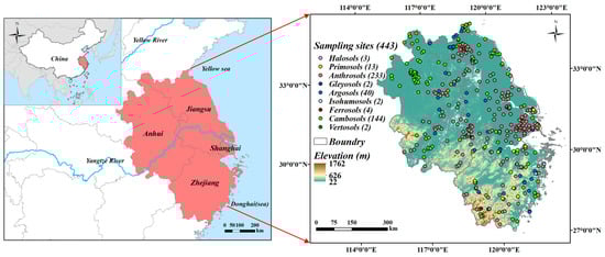
Figure 1.
The location of the study area (left) and the sampling sites (right). Sampling sites are classified and named according to the Chinese Soil Taxonomy.
The data for this study originate from the systematic survey results of soil taxa and soil series based on the Chinese Soil Taxonomy system. Specifically, the data were sourced from the volumes of the “Soil Series of China” series dedicated to Jiangsu Province [27], Zhejiang Province [28], Anhui Province [29], and Shanghai Municipality [30]. The soil profile surveys were conducted from 2009 to 2013. The “Soil Series of China” was compiled through a decade-long systematic investigation conducted by the Institute of Soil Science, Chinese Academy of Sciences (ISSCAS), in collaboration with numerous universities and research institutions across China. The data were collected by the research team following a unified sampling protocol and field investigation standards and were complemented by laboratory soil sample analyses. The data also took into account soil types, distribution area, spatial uniformity, and intensively sampled points in typical regions, ensuring high data quality and strong representativeness. The database’s high reliability and systematic nature make it the most important source of soil survey information in China since the second national soil survey, and it has been widely applied in soil science and related fields of research [31,32,33]. The collected data provide detailed information about the soil conditions in the study area, including soil types, geographic locations, horizon divisions, organic matter content, texture, BD, pH, and the >2 mm gravel content of the soil profiles. After screening and processing, a total of 443 representative soil profiles were selected for analysis, comprising 143 profiles from Jiangsu Province, 114 from Anhui Province, 47 from Shanghai Municipality, and 139 from Zhejiang Province (Figure 1). These profiles cover nine soil orders according to the Chinese Soil Taxonomy [34], including Vertosols, Cambosols, Ferrosols, Isohumosols, Argosols, Gleyosols, Anthrosols, Primosols, and Halosols. Additionally, we provided a cross-reference table (Table S1) for the classification units of the sampled profiles in both the Chinese Soil Taxonomy (CST) and the World Reference Base for Soil Resources (WRB) [35]. A total of 1929 soil horizon samples were collected from the 443 profiles.
At each sampling site, undisturbed soil cores were collected from the center of each soil horizon using standard sharpened steel cylinders of 100 cm3 volume (5.05 cm diameter, 5 cm height), with three replicates taken from each soil horizon to measure soil BD. At the same time, disturbed soil samples weighing approximately 2–3 kg were collected from each horizon using individual plastic or cloth bags to determine soil particle composition and organic carbon content.
The undisturbed soil core samples were weighed in the field and then brought back to the laboratory for drying in a 105 °C oven until constant weight (>48 h). The dried soil blocks inside the steel cylinders were weighed, and then they were sieved through a 2 mm mesh, after which the portion > 2 mm was weighed. The soil BD values were calculated, i.e., the mass of an oven-dried sample of undisturbed soil per unit bulk volume [36], using the following formula [37]:
where represents the bulk density of the soil (<2 mm fine earth fraction) (g cm−3); represents the oven-dry weight of the soil block inside the steel cylinder (g); represents the dry weight of the gravel inside the steel cylinder (g); represents the volume of the steel cylinder (cm3); denotes the volume of the gravel inside the steel cylinder (cm3), where 2.65 is the specific gravity of gravel (g cm−3) [38].
Before the analysis of soil chemical properties, disturbed soil samples were spread out on trays to remove plant roots, stems, and other intrusive materials such as bricks and tiles. The samples were air-dried at 30–35 °C and then crushed and sieved. Soil particle composition was determined using the pipette method, and according to the USDA soil classification system, soil texture is classified into three fractions: clay (<0.002 mm), silt (0.002–0.05 mm), and sand (0.05–2 mm). SOC content was measured using the potassium dichromate–sulfuric acid digestion method [39].
2.2. SOCD Calculation
SOCD refers to the stock of SOC in a unit area (1 m2 or 1 hm2) and a specific depth (typically 1 m) of the soil horizon. Equation (2) is used to compute SOCDicm (kg m−2) for each horizon within a soil profile, representing the stock of SOC within a 1 cm thick layer per unit area:
The SOCD of soil horizon i (SOCDi) (kg m−2) can be calculated using Equation (3) (assuming that the SOCDicm value per centimeter is consistent within the soil horizon):
The SOCD within a soil profile (kg m−2) can be calculated using Equation (4):
where n represents the number of soil horizons, SOCi denotes the SOC content (g kg−1) of soil horizon i, BDi is the soil bulk density (g cm−3) of soil horizon i, Di stands for the thickness (cm) of soil horizon i, Ci represents the content of gravel (>2 mm) in the soil sample for that horizon (%), and 100 is a unit conversion factor.
2.3. SOCD Estimation
2.3.1. The Novel Method Proposed in This Paper
Considering the availability of gravel content data, two new methods were employed in this study to estimate SOCD.
Method one: When gravel content data were missing, linear, polynomial, and power function regression models were separately established for SOC and SOCDicm. The specific formulas are as follows:
Method two: When gravel content data were available, they were utilized as a correction factor. Linear, polynomial, and power function regression models were separately established for SOC, gravel content, and SOCDicm. The specific formulas are as follows:
where a, b, and c are calibration coefficients.
These regression models intuitively describe the mathematical relationships between SOC, gravel content, and SOCDicm. The linear regression model is the most basic, making it suitable for simple linear relationships. The polynomial regression model can capture potential nonlinear relationships, making it suitable for more complex data distributions. The power function regression model is particularly useful for describing power law relationships between variables, especially in cases of nonlinear growth or decay trends. These three models are easy to interpret, computationally efficient, and capable of covering a range of relationships from simple linear to complex nonlinear. They provide a reliable mathematical foundation for SOCD estimation, with parameters that are easy to calibrate, offering high practicality and operability.
SOCDi can be obtained by multiplying SOCDicm by the thickness of soil horizon i, denoted as Di (Equation (3)).
In a soil profile with n soil horizons, the total SOCD of the profile is obtained by summing the SOCDi of each horizon (Equation (4)).
Equations (3)–(10) demonstrate that if SOC can be used to estimate SOCDicm accurately, it would enable the calculation of precise SOCD.
2.3.2. Traditional BD Substitution Methods
To validate the accuracy advantage of the proposed method in SOCD estimation, we designed a comparative experiment using eight traditional BD substitution methods (including a mean method, a median method, and six PTFs) as references (Table 1). M1 and M2, respectively, used the mean and median of measured BD values for estimation. Experience has shown that SOC or soil organic matter (SOM) and soil texture are the main factors determining soil BD. Based on SOC or SOM and texture data, numerous attempts have been made to estimate soil BD using PTFs [40]. We selected six commonly used PTFs for estimating BD, denoted as M3, M4, M5, M6, M7, and M8. Among them, M3 to M6 were established based on the relationship between BD and SOC/SOM to estimate BD, while M7 and M8 used SOC and soil texture as independent variables for BD estimation. Subsequently, the estimated BD values obtained above were used in Equation (2) to calculate the SOCDicm values, which were further calculated from Equations (3) and (4) to obtain SOCD values. By comparing the estimation results of these traditional methods with those of the proposed method, we comprehensively assessed the applicability and accuracy of the new approach, highlighting its advantages in SOCD estimation.

Table 1.
Methods used to estimate soil BD.
2.4. Data Splitting
The dataset was divided on a complete profile basis, with 300 profiles (approximately 67.72%) randomly selected as the calibration set (including 1309 soil horizon samples), while the remaining 143 profiles (approximately 32.28%) were allocated as the prediction set (including 620 soil horizon samples). Within the profiles of the calibration set, models were established using all soil horizon samples. Subsequently, the constructed models were validated for their predictive capability on independent samples from the soil horizons of the prediction set profiles. All calibration and prediction processes were carried out in MATLAB 2022a (MathWorks Inc., Natick, MA, USA).
2.5. Evaluation of Model Performance
In this article, the predictive models were evaluated through three statistical metrics calculated between the predicted values and the measured values: the root mean square error (RMSE), coefficient of determination (R2), and the ratio of performance to interquartile distance (RPIQ).
The lower the RMSE, the closer the R2 is to 1, and the higher the RPIQ, the better the model. The coefficient of determination and root mean square error for the calibration set are denoted as Rc2 and RMSEC, respectively, while for the prediction set, they are Rp2 and RMSEP. The RPIQ is the ratio of IQ to RMSEP, where IQ represents the interquartile range (IQR) of the measured values, which is the difference between the third quartile (Q75) and the first quartile (Q25) of the sample values; in other words, it is the range where values fall between 25% and 75% of the ordered data. The RPIQ, an improvement over RPD in model evaluation, overcomes the bias from non-normal data distributions by considering quartile differences [45,46,47].
2.6. Statistical Analysis
The correlations between soil properties were discerned using Spearman correlation analysis and partial correlation analysis. The assumption of normality in the data was tested using the Kolmogorov–Smirnov (K–S) test. For non-normally distributed original data, the Kruskal–Wallis H test was employed to test for significant differences (p < 0.05). Further intergroup differences were analyzed using the Bonferroni multiple mean comparison method (p < 0.05). The aforementioned data analysis procedures were performed using OriginPRO 2021, SPSS (IBM Version 21, Chicago, IL, USA), and R version 4.3.1 [48]. The partial correlation coefficients were computed using the R package ppcor [49]. The relative deviation of SOCDicm obtained from the measured method and the new method proposed in this study was calculated to explore the impact of gravel content on SOCD. The relative deviation was calculated by taking the absolute difference between the two sets of data, dividing it by the sum of the two sets of data, and then multiplying by 100%. This calculation process was performed in MATLAB 2022a (MathWorks Inc., MA, USA).
3. Results
3.1. The Basic Statistics of the Dataset
Descriptive statistics were calculated for soil properties on all samples and the calibration and prediction sets (Table 2). Overall, BD ranged from 0.58 to 1.80 g cm−3, with a mean of 1.37 g cm−3 and a standard deviation of 0.19 g cm−3. BD exhibited the lowest variation (14%) compared to other soil variables. The SOC content was relatively low, with an average of 7.87 g kg−1 and the highest variation (CV = 86%), ranging from 0.06 to 52.37 g kg−1. The heterogeneity of SOCDicm, calculated based on measured BD values, was 74%, second only to that of SOC. The profile SOCD was calculated using Equation (4), ranging from a maximum of 24.07 kg m−2 to a minimum of only 0.08 kg m−2, with a standard deviation of 3.75 kg m−2. Data follow a normal distribution when skewness and kurtosis are both 0. However, SOC, SOCDicm, SOCD, sand, and clay exhibited positive skewness and either leptokurtic or platykurtic distributions, while BD and silt displayed negative skewness. This suggests that the soil property data have a non-normal distribution. Similar statistical values were observed for various soil properties in the calibration, prediction, and overall datasets, indicating a fairly even data distribution between the two sets.
Table 2.
Descriptive statistics for soil properties.
3.2. Correlation Analysis
The correlation analysis results indicated that BD was significantly correlated with SOC, SOCDicm, sand, and clay at the 0.001 level while showing a weak correlation with silt (p > 0.05). The relationship between BD and SOC was the closest, and BD was also closely associated with soil texture. SOCDicm was significantly negatively correlated with BD and sand but significantly positively correlated with SOC, silt, and clay. The highest correlation was observed between SOC and SOCDicm (r = 0.976), followed by that between sand and silt (r = −0.799), BD and SOC (r = −0.553), sand and clay (r = −0.431), and BD and SOCDicm (r = −0.410). From the correlation analysis results, it is evident that the correlation between SOC and SOCDicm is more robust than that between BD and SOC, as well as soil texture. This suggests that predictive models established based on SOC and SOCDicm might exhibit higher accuracy than BD PTFs developed with SOC and soil texture as independent variables.
Due to the significant correlation between SOC and BD (r = −0.553), it was necessary to compute the partial correlation coefficients of SOCDicm with both SOC and BD. After removing the influence of SOC, the correlation between BD and SOCDicm underwent a significant change. The correlation coefficient between BD and SOCDicm shifted from −0.410 to 0.715, indicating that the correlation was enhanced and changed from negative to positive. After eliminating the effects of BD, the correlation between SOC and SOCDicm remained significantly positive, and the correlation coefficient increased from 0.976 to 0.986.
3.3. The Direct Estimation of SOCD Based on the Novel Method
3.3.1. Estimation Results of SOCDicm Without Considering Gravel Content
We generated a scatter plot of SOC against the measured SOCDicm using the calibration set and performed separate fittings using linear, polynomial, and power functions (Figure 2). All three function fittings resulted in R2 values surpassing 0.91, indicating a robust functional relationship between SOC and SOCDicm. Interestingly, the results demonstrated that the outcomes of the nonlinear fitting slightly outperformed those of the linear fitting.

Figure 2.
The scatter plot and fitting results of the calibration subset for SOC and SOCDicm. m represents the number of soil horizon samples.
The prediction set SOC values were employed to generate predicted SOCDicm values using the three models above. A scatter plot (Figure 3) was constructed to compare the predicted SOCDicm values from the prediction set with the actual measured SOCDicm values. The SOCDicm predictions from all three regression models exhibited favorable alignment with the actual measured values (Rp2 > 0.9), albeit demonstrating a certain degree of underestimation for low values and overestimation for high values. The polynomial regression model showed the highest prediction accuracy, with Rp2 and RMSEP values of 0.919 and 0.019 kg m−2, respectively, and an RPIQ value of 4.357. Comparatively, the predictive accuracy of the linear regression model and power function regression model was inferior to that of the polynomial regression model. Furthermore, the results of these two models were comparable, with Rp2 values of 0.901 and 0.911 and RPIQ values of 3.929 and 3.942, respectively. The above results indicated that utilizing SOC enables a highly effective direct prediction of SOCDicm.
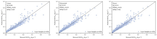
Figure 3.
A comparison between the measured and predicted SOCDicm values in the prediction subset without considering gravel content. m represents the number of soil horizon samples.
A thorough analysis of the significance of differences was conducted on the predicted outcomes of the three fitting methods to assess whether significant differences exist in the predictive capabilities of the three distinct fitting models. The results (Figure 4) indicated that there were no statistically significant differences (p > 0.05) in the estimated SOCDicm values obtained from the three fitting methods, implying comparable predictive accuracy across the models. Moreover, the estimated SOCDicm values from all three models aligned closely with the measured values, demonstrating high prediction accuracy and reliability.
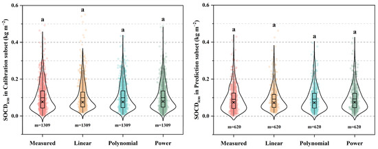
Figure 4.
Violin plots of SOCDicm estimated by different models without considering gravel content. Boxes represent interquartile ranges, with the upper and lower edges corresponding to the third quartile (Q3) and first quartile (Q1), respectively. The solid line inside the box marks the median (Q2), while the cross symbol (×) represents the mean. The “whiskers” outside the box indicate the data range, extending to the maximum and minimum values; values beyond this range are considered outliers. The kernel density estimation curve illustrates the probability distribution of the data across different intervals, with its width indicating data density—the wider the curve, the more concentrated the data. The points represent the measured or predicted SOCDicm values of all soil horizon samples. m represents the number of soil horizon samples. Different letters indicate significant differences among different models (p < 0.05).
3.3.2. Estimation Results of SOCD Without Considering Gravel Content
The profile SOCD was calculated from the SOCDicm estimated by the three models in the calibration and prediction sets (Equations (3) and (4)). Scatter plots (Figure 5) were generated to compare the estimated SOCD with the actual measured SOCD. The three established models could all be employed for SOCD estimation, with Rc2 ranging from 0.860 to 0.877; Rp2 ranging from 0.869 to 0.893; RMSEC and RMSEP varying between 1.346 and 1.434 kg m−2 and 1.147 and 1.270 kg m−2, respectively; and RPIQ ranging from 3.568 to 3.948. The polynomial regression model exhibited superior results (the highest Rc2, Rp2, and RPIQ values, as well as the smallest RMSEC and RMSEP). The linear regression model demonstrated higher modeling precision than the power function regression model, although its validation accuracy was relatively lower. While the calibration set results tended to underestimate lower values, this phenomenon was less pronounced in the prediction set. These outcomes suggest that the SOCDicm predictions derived from SOC can be effectively utilized for profile SOCD calculations, yielding favorable results.
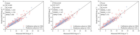
Figure 5.
The estimated SOCD results without considering the gravel content. n represents the number of soil profiles.
The significance analysis of the differences indicated no significant variation in estimated SOCD among different models (p > 0.05). The SOCD values estimated from the three models were not significantly higher or lower than the measured SOCD values; thus, these models demonstrated similar accuracy in SOCD estimation (Figure 6).
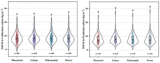
Figure 6.
Violin plots of SOCD estimated by different models without considering gravel content. Boxes represent interquartile ranges, with the upper and lower edges corresponding to the third quartile (Q3) and first quartile (Q1), respectively. The solid line inside the box marks the median (Q2), while the cross symbol (×) represents the mean. The “whiskers” outside the box indicate the data range, extending to the maximum and minimum values; values beyond this range are considered outliers. The kernel density estimation curve illustrates the probability distribution of the data across different intervals, with its width indicating data density—the wider the curve, the more concentrated the data. The points represent the measured or predicted SOCD values of all soil profiles. n represents the number of soil profiles. Different letters indicate significant differences among different models (p < 0.05).
3.3.3. The Impact of Gravel Content on the Estimation of SOCDicm
Dividing soil sample data based on gravel content, the discrepancies between the measured values of SOCDicm and the estimated values obtained from three modeling methods generally increased with an increase in gravel content (Figure 7). When the gravel content was less than 5%, there was no significant difference among the methods, and all three models slightly underestimated SOCDicm. When the gravel content was between 5% and 30%, the differences between the measured values of SOCDicm and the estimates from the three models were not significant, and the underestimation phenomenon transitioned to overestimation. Conversely, when the gravel content was greater than or equal to 30%, the discrepancies between the results of the three modeling methods and the measured values were considerable (Figure 7).

Figure 7.
The differences in SOCDicm among different gravel content levels between the three modeling methods and the measured method. Different letters indicate significant differences among different models (p < 0.05).
The systematic errors of the three new models in estimating SOCDicm are represented by the relative deviation between the estimated values and the measured results. In the highest gravel content category (≥30% gravel content) of soil samples, the linear regression model exhibited the largest deviation, with an average overestimation of SOCDicm by 34.77%, while the polynomial and power function regression models overestimated by 32.84% and 33.78%, respectively (Table 3). In this study, the gravel content of most soil horizons (76.72%) was less than 5%, with those without gravel content accounting for 62.52% of the total. Overall, disregarding gravel content resulted in an overestimation of SOCDicm by 7.01–9.45% (Table 3).
Table 3.
Proportion of different gravel content levels and average relative deviation of SOCDicm estimated by different modeling methods compared to measured SOCDicm values.
3.3.4. The Estimation Results of SOCDicm with Gravel Content as a Correction Factor
Linear, polynomial, and power function regression models were separately established with SOC and gravel content as predictor variables, and the estimation ability of these models was verified. The results (Table 4, Figure 2 and Figure 3) indicated that considering gravel content improved the accuracy of the SOCDicm estimation models, with an increase in R2 ranging from 0.028 to 0.036 and RPIQ reaching 4.852 to 5.397. The power function regression model exhibited the strongest estimation capability for SOCDicm, followed by the polynomial regression model, while the linear regression model had the poorest estimation capability. There were minimal differences in the SOCDicm estimation results among different modeling methods (Figure 8), and no significant discrepancies were observed compared to the measured values, indicating that the model predictions are reasonably reliable.
Table 4.
The specific models and prediction results for estimating SOCDicm based on SOC and gravel content.
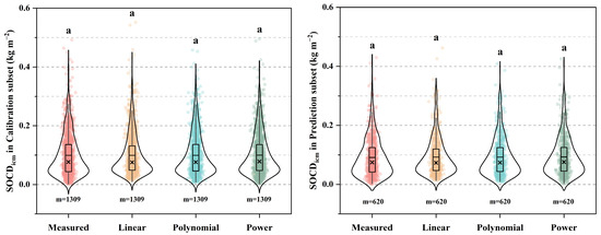
Figure 8.
Violin plots of SOCDicm estimated by different models considering gravel content. Boxes represent interquartile ranges, with the upper and lower edges corresponding to the third quartile (Q3) and first quartile (Q1), respectively. The solid line inside the box marks the median (Q2), while the cross symbol (×) represents the mean. The “whiskers” outside the box indicate the data range, extending to the maximum and minimum values; values beyond this range are considered outliers. The kernel density estimation curve illustrates the probability distribution of the data across different intervals, with its width indicating data density—the wider the curve, the more concentrated the data. The points represent the measured or predicted SOCDicm values of all soil horizon samples. m represents the number of soil horizon samples. Different letters indicate significant differences among different models (p < 0.05).
3.3.5. The Estimation Results of SOCD with Gravel Content as a Correction Factor
The SOCDicm values estimated by the three models using the calibration and prediction subsets were used to calculate the profile SOCD (Equations (3) and (4)). Scatter plots of the estimated SOCD against the measured SOCD were drawn (Figure 9). The SOCD estimation values obtained from all three models demonstrated good agreement with the measured values. The inclusion of gravel content data resulted in the predicted values being more concentrated and symmetrically distributed around the 1:1 line. Among the models, the polynomial regression model exhibited the best performance. The values of Rc2 ranged from 0.938 to 0.946; Rp2 ranged from 0.927 to 0.945; RMSEC and RMSEP varied between 0.889 and 0.959 kg m−2 and 0.819 and 0.949 kg m−2, respectively; and RPIQ ranged from 4.773 to 5.533. These results indicated that considering gravel content as a correction factor for estimating SOCD results in high precision and good performance. The SOCD estimation results from the three models were close to the true values, with no significant differences observed, demonstrating their ability to accurately estimate SOCD values (Figure 10).
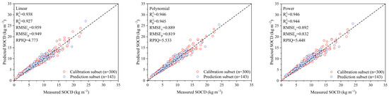
Figure 9.
The estimated SOCD results considering the gravel content. n represents the number of soil profiles.
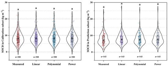
Figure 10.
Violin plots of SOCD estimated by different models considering gravel content. Boxes represent interquartile ranges, with the upper and lower edges corresponding to the third quartile (Q3) and first quartile (Q1), respectively. The solid line inside the box marks the median (Q2), while the cross symbol (×) represents the mean. The “whiskers” outside the box indicate the data range, extending to the maximum and minimum values; values beyond this range are considered outliers. The kernel density estimation curve illustrates the probability distribution of the data across different intervals, with its width indicating data density—the wider the curve, the more concentrated the data. The points represent the measured or predicted SOCD values of all soil profiles. n represents the number of soil profiles. Different letters indicate significant differences among different models (p < 0.05).
3.4. Estimating SOCD Based on Traditional BD Substitution Methods
3.4.1. Estimation Results of BD Based on PTFs
The parameters of the six published PTFs in Table 1 were calibrated (Table 5) to predict BD values. The R2 values of the PTFs ranged from 0.332 to 0.372, RMSE values ranged from 0.143 to 0.154 g cm−3, and RPIQ values ranged from 1.786 to 1.822 (Table 6). The performance of M7 and M8 was slightly better than that of other PTFs, with the highest Rp2 and RPIQ values and the lowest RMSE values. The validation accuracy of M3 and M4 was slightly lower, and the predictive accuracy of all models showed little difference. These results suggest that considering soil texture along with SOC can improve the predictive accuracy of the model to some extent.
Table 5.
Summary of revised PTFs defined in previous research.
Table 6.
The accuracy of PTFs for BD estimation.
3.4.2. Results of SOCDicm Based on Estimated BD
Based on the soil sample data from the study area, the mean and median values of BD were calculated to be 1.37 and 1.40 g cm−3, respectively. The BD values obtained from the mean, median, and the six PTFs were individually incorporated into Equation (2) to compute the predicted values of SOCDicm, which were then compared with the measured SOCDicm. As shown in Table 7, the predicted SOCDicm values from the six PTF models were closely aligned and demonstrated high precision. The values of Rc2 and Rp2 ranged from 0.941 to 0.958 and 0.947 to 0.950, respectively. The RMSEC and RMSEP values fell between 0.015 and 0.018 kg m−2, while the RPIQ ranged from a minimum of 5.400 to a maximum of 5.523. Despite the relatively low predictive accuracy of BD PTFs (Table 6), the precision of SOCDicm was high. In comparison, while the accuracy of estimating SOCDicm using the mean and median values of BD was relatively low, it still yielded satisfactory results (R2 ≥ 0.830).
Table 7.
The predicted SOCDicm results of the eight traditional methods.
3.4.3. Results of SOCD Based on Estimated BD
The predicted SOCDicm was multiplied by the respective thickness of each soil horizon to calculate SOCDi (Equation (3)), and then the profile SOCD was calculated from SOCDi (Equation (4)). The predicted SOCD was plotted against the measured SOCD in a scatter plot (Figure 11). It can be observed that the accuracy of the SOCD predicted based on BD PTFs is quite similar to that of SOCDicm. The values of Rp2 were greater than 0.948, the RMSEP values were less than 0.796 kg m−2, and the RPIQ values ranged from 5.689 to 5.805. Although M7 and M8 exhibited the strongest predictive capability for BD, their predictive results for SOCD were not optimal, probably because M3 to M6 more effectively captured the relationship between SOC/SOM and SOCD, while M7 and M8 did not fully consider the complex relationship between SOC and BD when predicting SOCD. Therefore, the predictive accuracy of SOCD is not directly correlated with the predictive accuracy of the PTFs. The SOCD prediction accuracy of M1 and M2 was relatively low.
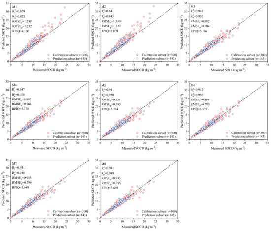
Figure 11.
The predicted SOCD results of the eight traditional methods. n represents the number of soil profiles.
4. Discussion
4.1. Correlation Between SOC, BD, and SOCDicm
Soil BD is primarily determined by the respective specific gravity and relative proportion of solid organic and inorganic particles, as well as the soil porosity. Due to the significantly lower density of organic matter compared to mineral particles, and its aggregation effect on soil structure, organic matter predominantly influences soil BD. Generally, an increase in organic matter content results in a decrease in BD and vice versa [50]. Therefore, soils rich in organic matter with a loose porous structure tend to have lower BD, while those with lower organic matter content and more compact structures have higher BD. SOC, SOM, and their correlation with BD are commonly used for carbon sink estimation [51]. Typically, SOC exhibits a negative correlation with BD [12,23,52], with higher SOC content leading to lower BD. This is because SOC reflects the organic matter content in the soil, which increases the interstitial space between soil solid particles due to its low density, enhancing soil aggregation and resulting in a decrease in soil BD [44]. Based on these factors, SOC becomes a crucial variable for constructing BD PTFs [9,25]. However, it is important to note that SOC is not always strongly correlated with BD. In soils with low SOC content, factors such as soil texture or other variables might primarily contribute to BD [41,42,53,54]. Research has shown that despite employing various simulation methods, predicting BD through PTFs remains challenging and often falls short of achieving satisfactory predictive levels [17].
According to Equation (2), theoretically, SOCDicm should exhibit a positive correlation with both SOC and BD. However, Spearman’s correlation coefficient revealed a negative correlation between SOCDicm and BD, which stems from the negative correlation between SOC and BD. Specifically, while SOC is positively correlated with SOCDicm, it is negatively correlated with BD, resulting in a negative correlation between BD and SOCDicm. Upon controlling for the influence of SOC, the relationship between BD and SOCDicm transitioned from negative to positive, and the correlation strengthened significantly. Interestingly, even after removing the influence of BD, the correlation between SOC and SOCDicm remained significantly positive, with a slight increase in the correlation coefficient. This suggests that SOC is the primary driving factor affecting SOCDicm, and the robust correlation between SOC and SOCDicm underlies the mechanism of directly estimating SOCDicm using SOC.
4.2. The Selection and Accuracy of BD PTFs
Many studies have indicated that BD is closely related to SOC or SOM and soil texture [40,55], and SOC or SOM and soil texture (sand, silt, and clay contents) were the most commonly used predictors in the literature when developing PTFs [56]. In our dataset, SOC, SOM, and soil texture are easily measurable and obtainable, whereas factors such as pH [17,57], CaCO3, cation exchange capacity [17,58], moisture content [52,59], and terrain features (elevation, slope, aspect) have been less frequently applied in previous PTFs and are not consistently available. The results of correlation analysis further confirm that BD is significantly correlated with SOC and is influenced by soil texture. Therefore, PTFs containing SOC and soil texture perform better than those containing only SOC. This is consistent with the findings of Bernoux et al. [54], Kaur et al. [40], and Tomasella and Hodnett [60]. Several studies recommended using SOC or SOM as the sole predictor for BD to avoid collinearity risks with other predictors [9,25,61,62,63]. Based on this, our study selected two categories of published PTFs (the first category using only SOC or SOM as a predictor and the second category incorporating SOC and soil texture together) and revised these PTFs to better fit the local soil data for estimating BD values.
Previous studies on BD PTFs have often been limited to analyzing the accuracy of predicting BD, with the determination coefficients (R2) of the established PTFs typically being less than 0.8. In addition, research regarding the further use of these PTFs for estimating SOCD is scarce. For instance, Chen et al. [9] utilized the generalized boosted model (GBM) algorithm to establish BD PTFs with an R2 less than 0.648. Similarly, the BD PTFs developed by Zheng et al. [21] exhibited accuracies below 0.775. The accuracy of BD PTFs is influenced by various factors, including modeling methods, the number of variables, and the composition of the modeling dataset [64]. For example, Al-Qinna and Jaber [44] suggested that incorporating nonlinear models or machine learning methods, as well as increasing the number of variables such as SOC, could potentially enhance the accuracy of prediction models. However, certain studies have indicated that increasing model complexity cannot effectively improve the precision of BD prediction models [21,65]. Developing BD PTFs based on regional or soil-type subdivisions could potentially enhance predictive accuracy to some extent [66,67]. In this study, the accuracy of the six PTFs for predicting BD was not high (Rp2 ≤ 0.358) (Table 6). This might be attributed to the diverse range of soil types covered by the samples and the use of traditional modeling methods. Additionally, other factors, such as sampling depth and pH, can also influence BD values. If these factors were incorporated as predictive variables, the performance of the PTFs could potentially be enhanced [20].
4.3. Model Accuracy Validation
Some studies utilized PTFs to estimate BD for calculating SOCD or SOC stocks, yet they did not provide the precision of the constructed PTFs. For instance, Xu et al. [10] developed three PTFs to estimate SOCD, with R2 values ranging from 0.850 to 0.917, which is lower than the accuracy achieved by the BD PTFs used in this study. Wiesmeier et al. [68] reported that applying BD PTFs led to an overestimation of SOC stocks by 20–50%. Xu et al. [24] highlighted the variability in PTFs as a significant source of uncertainty in SOC stock estimation, and this uncertainty was exceptionally high for soils with low or high SOC content. In this study, a systematic comparison of the accuracy of BD PTFs and their estimated SOCD was conducted. The results showed that the R2 values for the BD PTFs were lower than 0.4 (Table 6). However, when these BD PTFs were used to calculate SOCDicm and then aggregated to SOCD, the determination coefficients for SOCDicm and SOCD were greater than 0.93 (Table 7 and Figure 11). This discrepancy can be attributed to the fact that when the BD PTF models built solely based on the single variable SOC are applied to Equation (2), they essentially embody the relationship between SOC, gravel content, and SOCDicm. Particularly for samples without gravel content, SOCDicm is solely determined by SOC. The strong correlation between SOC and SOCDicm determines the high accuracy of SOCDicm estimation. Although M7 and M8 include texture data, the correlation between texture and SOCDicm is relatively weak, and the contribution of texture data in the model is minor (Table 6). The incorporation of texture data did not significantly enhance the accuracy of SOCD estimation. This suggests that the computation of SOCD is intricate, and the superior performance of BD PTFs does not necessarily guarantee the highest accuracy in predicting SOCD.
This study found that in estimating SOCD, the accuracy of the BD PTF method surpassed that of the mean and median methods (Figure 12). For certain soil types, changes in the natural environment and land use can significantly influence their physicochemical properties [12,69,70,71,72]. Additionally, the mean and median methods are greatly affected by the representativeness of soil sampling [10]. Therefore, the mean and median methods overlook external factors’ impacts on BD, leading to higher uncertainty in SOCD estimation. In contrast, PTFs consider the relationship between BD and soil physicochemical properties, thus offering higher accuracy. Furthermore, this study found that directly estimating SOCDicm from SOC was less accurate than the BD PTF method (Figure 12). Part of the reason for this is that the process of calculating SOCDicm by substituting BD PTFs into Equation (2) considers the gravel content factor, whereas the calculation process of directly estimating SOCDicm from SOC ignores this factor (Equations (5)–(7)), leading to increased errors. Gravel content is one of the primary parameters for estimating SOCD and soil carbon pools. However, gravel content information is not always available, and rock fragment components are often overlooked in regional-scale studies or national soil surveys [68], making it a significant limiting factor for carbon stocks and concentration [73,74]. The presence of gravel in soil occupies the volume originally composed of fine earth [75], altering soil physicochemical properties such as BD [76,77,78,79] and carbon stocks. Additionally, the content, porosity, and distribution of gravel in soil further alter its physical properties (such as BD and pore distribution). These changes, by affecting soil’s hydrological processes, heat transfer, and other intermediary processes, indirectly or directly alter the soil carbon cycle and SOCD [80]. Therefore, the relationship between gravel content and SOCD is multidimensional, reflecting both its direct impact on soil physical properties and its effect on the dynamics of SOCD through the regulation of carbon cycling processes. Previous studies have shown that neglecting gravel content led to the overestimation of measured soil carbon pools [11,26,75], especially for soils rich in gravel content [12]. The results of this study are consistent with this finding, indicating that ignoring the influence of gravel content resulted in an overall overestimation of SOCDicm by 7.01–9.45%. Particularly, for soils with a gravel content ≥ 30%, gravel content is particularly important for accurately determining SOCD. The soils in the Yangtze River Delta region are mainly formed by sedimentation from rivers, lakes, and seas, and they are also influenced by other parent materials such as loess, quaternary red soil, weathered residual materials, and colluvium. Due to these specific parent materials, the gravel content in the soils of this region is relatively low. Therefore, even without considering gravel content, the impact on SOCD is not significant. In cases of missing gravel content data, we can still estimate SOCD quickly and accurately. By introducing gravel content data into Equations (8)–(10), the accuracy of SOCDicm estimation was improved, making this correction comparable to the BD PTF method in terms of SOCD estimation ability and exhibiting higher precision compared to using the BD mean and median substitution methods (Figure 12). The inclusion of gravel content as a correction factor significantly improved the estimation accuracy of SOCD. Specifically, the model’s Rc2 and Rp2 increased from 0.860–0.877 to 0.938–0.946 and from 0.869–0.893 to 0.927–0.945, respectively, while RMSEC and RMSEP decreased by 0.457–0.542 kg m−2 and 0.321–0.387 kg m−2, respectively. The RPIQ increased from 3.568–3.948 to 4.773–5.533 (Figure 5 and Figure 9). When gravel content is not considered, directly estimating SOCD from SOC may lead to the overestimation of carbon density, especially in soils with high gravel content. After incorporating the gravel content factor, the model automatically corrected this error, enhancing estimation accuracy. Gravel content varies significantly across different pedogenic environments and land use types. Without correction, it is assumed that the influence of SOC on SOCD is consistent across all soils, whereas the correction allows the model to adjust SOCD based on gravel content, thus improving its applicability to different soil types. This study recommends using the gravel correction factor method to estimate SOCD, avoiding the overestimation of the SOC pool and enabling a more scientific assessment of soil carbon sequestration function. This improvement is especially applicable to soils with higher gravel content, highlighting the importance of determining gravel content and incorporating it into the model in future studies, particularly in regions with high gravel content, to enhance SOCD estimation accuracy. However, when gravel content data are difficult to obtain, the method proposed in this study, which directly estimates SOCDicm based on SOC, still holds significant potential for application, providing a feasible solution for SOCD estimation in the absence of gravel data and broadening the applicability of the method. It is worth noting that this study did not actually measure gravel density but used 2.65 g cm−3 as a substitute, which may introduce biases in estimating fine earth BD and organic carbon pools [81].
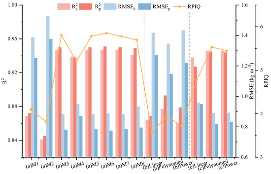
Figure 12.
Comparison of SOCD estimation accuracy: (a) eight traditional methods vs. (b) novel method without considering gravel content vs. (c) novel method considering gravel content. Vertical dashed lines serve as subplot demarcations, separating the three comparative analysis sections: (a), (b), and (c).
Other methods for directly estimating SOCD without requiring SOC data have also been explored. For example, Song et al. [82] and Sun et al. [83], respectively, utilized environmental variables such as terrain and annual average precipitation to directly estimate SOCD. However, these methods are complex and have lower R2 values compared to the results of this study (R2 = 0.87). Liu et al. [4] employed soil spectra combined with deep neural network technology to estimate SOCD, with the best R2 being less than 0.81. While this method can be used for small-scale spatial mapping, it still requires the measurement of soil spectral data. The new method proposed in this study effectively captures the strong correlation between SOC and SOCDicm. Although the precision of the results is slightly lower than that of the BD PTF method, the new method’s advantage lies in its clear and simple mechanism, making it suitable for the rapid estimation of SOCD for a large number of soil samples.
4.4. Comparison and Limitations of Soil Organic Carbon Measurement Methods
SOC is a major component of SOM. It includes microbial cells, plant and animal residues at various stages of decomposition, stable “humus” synthesized from these residues, and nearly inert, highly carbonized compounds such as charcoal, graphite, and coal [84]. Because it can be measured simply and efficiently, SOC is commonly employed as a key proxy indicator for determining SOM content [85].
Currently, SOC determination primarily utilizes two techniques: the wet digestion and dry combustion methods. The Walkley–Black (WB) wet digestion method has been widely adopted as the standard procedure in most soil testing laboratories due to its operational simplicity, low cost, and minimal equipment requirements [84]. The SOC data used in this study were obtained using this method from the “Soil Series of China”. However, extensive research has demonstrated that the WB method significantly underestimates SOC content [86,87,88,89,90,91,92], with marked spatial variability in organic carbon recovery rates. For instance, Krishan et al. [91] found that the WB method underestimated SOC by an average of 45% in Himalayan soils and 33% in central Indian soils. The lower recovery rate of SOC in soil may be attributed to the incomplete oxidation of organic carbon by the WB method. While a standard correction factor of 1.32 (assuming a 76% SOC recovery rate) is conventionally applied to convert Walkley–Black carbon (WBC) to total organic carbon (TOC), the assumed 76% recovery rate is generally overestimated. Actual recovery rates vary considerably depending on land use patterns, soil types, sampling depths, soil textures, organic matter characteristics, management practices, and climatic conditions [92,93,94]. Therefore, it is recommended to apply a differentiated recovery correction factor that accounts for the above factors to improve the accuracy of SOC estimation using the WB method.
In contrast, dry combustion methods (including the use of an elemental analyzer, TOC analyzer, and gas chromatograph) achieve nearly 100% carbon recovery and are internationally recognized as the most reliable standard for SOC determination [93]. Although minor variations exist among different dry combustion systems, their measurement precision significantly surpasses that of the wet digestion method [95]. Nevertheless, their widespread adoption in developing countries faces challenges including high equipment costs, specialized technical requirements, and environmental compliance issues [96]. This underscores the importance of developing universal conversion models that account for soil type, land use, and climate to accurately translate WBC to true TOC. Although strong correlations have been observed between WB and dry combustion results [93,97,98,99], the systematic bias of the WB method cannot be overlooked. Therefore, for applications requiring high precision (e.g., carbon sequestration accounting), dry combustion methods should be prioritized. If WB method data are used, it is recommended to apply soil-specific correction factors considering parameters such as texture, land use, and depth.
Loss on ignition (LOI) represents another simple method for SOM determination. One of the PTFs developed by Huntington et al. [41] was based on LOI-measured SOM [84]. However, LOI lacks a unified standard protocol, and its accuracy is influenced by factors such as furnace type, sample mass, duration, and the temperature of ignition and clay content of samples [100], potentially leading to SOM overestimation (due to water loss or mineral decomposition) or underestimation (from incomplete combustion) [92]. Davies [101] reported good consistency between SOM content determined by the WB and LOI methods. Therefore, in this study, SOM content was derived by multiplying WB-measured SOC values by 1.724.
Given that our SOC data were obtained using the Walkley–Black method, potential systematic underestimation should be acknowledged. Future research should prioritize dry combustion methods or develop context-specific correction models incorporating soil type, texture, and land use patterns to enhance SOC estimation accuracy.
4.5. The Applicability and Limitations of the Models
Geographical phenomena often exhibit regional characteristics, and statistical models constructed based on soil properties are more applicable within the specific regions covered by the modeling samples, making it challenging to generalize the model beyond the specific area or soil types [66,102,103]. The SOCDicm model developed in this study, based on SOC and incorporating gravel content as a correction factor, is suitable only for a limited geographical area. In this particular study area, the variation in the BD of soil samples is relatively small, which may contribute to the good results obtained by the new method. When the study scope extends to regions with more extensive variations in BD, the results may not meet expectations. In addition, this study’s SOCDicm model construction only considered SOC and gravel content and did not account for other factors that may influence SOCD estimation, such as soil type, land use type, climatic factors (e.g., temperature and precipitation), vegetation, soil microorganisms, parent material, topographical factors, soil physicochemical properties, and human activities [104]. The spatial variability in these factors may affect the model’s accuracy. Our decision to use only SOC and gravel content was based on two main considerations. First, to ensure the model’s generalizability and practicality, we prioritized the most reliable and widely available variables in the dataset. Additionally, to develop a simple and easily applicable method, we intentionally streamlined the model structure, focusing on SOC and gravel content as the two most explanatory variables. Incorporating too many variables could increase model complexity and reduce its applicability, particularly in regions where data acquisition is challenging. Second, factors such as climate, parent material, and topography require extensive data collection, making it difficult to obtain complete datasets, which limits their application in this study. To enhance the regional applicability and generalizability of the model, future research could incorporate these variables into the model and optimize relevant parameters. Moreover, refining variable selection strategies and optimizing model structures would further enhance the model’s interpretability and predictive accuracy. Constructing statistical models based on specific soil types can somewhat enhance accuracy [22,68], especially for larger study areas, where grouping by major soil types should be considered. In future research, national- or global-scale data can be used to establish estimation models for each soil type and evaluate their accuracy based on dividing the dataset according to soil type, thus providing high-precision estimation formulas for the SOCD estimation of various soil types and further verifying the reliability of the new method. With the development of computers and machine learning algorithms, SOCD estimation methods have evolved from basic linear and nonlinear regression models to data mining approaches. Simple and multiple linear regression models have been widely used and are often employed as benchmarks for comparison with other advanced methods. Some data mining methods, such as artificial neural networks, extreme gradient boosting, random forests, and support vector machines, have been used in recent SOCD-related studies [83]. However, machine learning methods typically require a large amount of training data, and their “black box” nature may reduce the interpretability of the results. Therefore, this study prioritizes traditional regression models, providing a transparent and easily interpretable computational framework. Future research can further explore the potential of machine learning methods in SOCD estimation.
5. Conclusions
This study proposed a novel method for estimating SOCD in the 0–100 cm soil profile of the Yangtze River Delta region in China, providing a feasible solution for SOCD estimation in the absence of BD data. Based on the availability of gravel content data, linear regression, polynomial regression, and power function regression were used to establish SOCDicm estimation models based on SOC and gravel content, and SOCD values were further calculated. This method has a clear mechanism and simple computation and avoids excessive reliance on BD data, effectively addressing the potential impact of incomplete gravel content data.
The results showed that in the absence of gravel content data, by leveraging the robust correlation between SOC and SOCDicm, SOC could be used to directly estimate SOCDicm with high accuracy and calculate the profile SOCD. The three function models demonstrated excellent predictive performance, with prediction set coefficients of determination (Rp2) exceeding 0.90, RMSEP below 0.021 kg m−2, and an RPIQ reaching up to 4.357.
Neglecting the effect of gravel content led to the overestimation of SOCDicm, with an overall overestimation range of 7.01–9.45%. In soils with a gravel content ≥ 30%, this overestimation was particularly significant, reaching 32.84–34.77%. By incorporating gravel content as a correction factor, the SOCD prediction accuracy of the model was further improved, with Rp2 increasing to 0.927–0.945, RMSEP decreasing to 0.819–0.949 kg m−2, and the RPIQ improving to 4.773–5.533. This highlights that gravel content is a critical factor influencing SOCD estimation accuracy, especially in high-gravel-content soils, where its correction effect plays a key role in enhancing model precision.
Compared to traditional BD substitution methods (BD mean method, BD median method, and BD PTF method), the proposed method exhibited significant advantages in SOCD estimation accuracy. The BD mean and median methods yielded an Rp2 ≤ 0.872, RMSEP ≥ 1.252 kg m−2, and an RPIQ between 3.809 and 4.100. The proposed method outperformed the BD mean and median methods in terms of SOCD estimation accuracy and was comparable to the BD PTF method, enabling reasonably accurate SOCD estimation.
The models developed in this study are based on soil data from the Yangtze River Delta region and are suitable for SOCD estimation in this area. However, due to differences in soil types, climatic conditions, and land use, the applicability of these models in other regions requires further validation. Future research could improve model applicability and scalability by incorporating additional variables such as climate, topography, soil types, and parent material. Additionally, region-specific estimation models could be developed for different soil types, and the potential of machine learning methods in SOCD estimation could be further explored.
The proposed method provides a novel approach to SOCD estimation in the absence of BD data. It offers new insights for calculating regional or global SOC stocks, contributing to the advancement of soil carbon estimation methodologies.
Supplementary Materials
The following supporting information can be downloaded at https://www.mdpi.com/article/10.3390/su17083533/s1, Table S1: Soil Orders in the Chinese Soil Taxonomy, and their approximate corresponding classes in World Reference Base for Soil Resources.
Author Contributions
Conceptualization, G.Z. and J.F.; Methodology, G.Z.; Software, J.F.; Validation, C.J., R.Z. and Y.Z.; Formal Analysis, Y.W.; Investigation, M.X.; Resources, G.Z.; Data Curation, J.F.; Writing—Original Draft Preparation, J.F.; Writing—Review and Editing, G.Z. and Y.Z.; Visualization, J.F.; Supervision, C.Z.; Project Administration, G.Z.; Funding Acquisition, G.Z. All authors have read and agreed to the published version of the manuscript.
Funding
This research was funded by the National Key R&D Program of China (Grant No. 2023YFE0208100), the National Natural Science Foundation of China (Grant No. 42371060), and the key project of the National Natural Science Foundation (Grant No. 42130405).
Institutional Review Board Statement
Not applicable.
Informed Consent Statement
Not applicable.
Data Availability Statement
The raw data supporting the conclusions of this article will be made available by the authors on request.
Acknowledgments
We would like to express our sincere gratitude to the editor and anonymous referees for their insightful and constructive comments.
Conflicts of Interest
The authors declare no conflicts of interest.
References
- Padarian, J.; Stockmann, U.; Minasny, B.; McBratney, A.B. Monitoring Changes in Global Soil Organic Carbon Stocks from Space. Remote Sens. Environ. 2022, 281, 113260. [Google Scholar] [CrossRef]
- Lal, R. Beyond COP 21: Potential and Challenges of the “4 per Thousand” Initiative. J. Soil Water Conserv. 2016, 71, 20A–25A. [Google Scholar] [CrossRef]
- Zhu, H.; Hu, W.; Ding, H.; Lv, C.; Bi, R. Scale- and Location-Specific Multivariate Controls of Topsoil Organic Carbon Density Depend on Landform Heterogeneity. CATENA 2021, 207, 105695. [Google Scholar] [CrossRef]
- Liu, Q.; He, L.; Guo, L.; Wang, M.; Deng, D.; Lv, P.; Wang, R.; Jia, Z.; Hu, Z.; Wu, G.; et al. Digital Mapping of Soil Organic Carbon Density Using Newly Developed Bare Soil Spectral Indices and Deep Neural Network. CATENA 2022, 219, 106603. [Google Scholar] [CrossRef]
- Sun, B.; Wang, Y.; Li, Z.; Gao, W.; Wu, J.; Li, C.; Song, Z.; Gao, Z. Estimating Soil Organic Carbon Density in the Otindag Sandy Land, Inner Mongolia, China, for Modelling Spatiotemporal Variations and Evaluating the Influences of Human Activities. CATENA 2019, 179, 85–97. [Google Scholar] [CrossRef]
- Jin, F.; Yang, H.; Zhao, Q. Research Progress on Soil Organic Carbon Storage and Influencing Factors. Soils 2000, 1, 12–18. [Google Scholar] [CrossRef]
- Wang, W. Spatial Distribution and Estimation of Topsoil Organic Carbon Density in Zhejiang Province. Master’s Thesis, Zhejiang University, Hangzhou, China, 2014. [Google Scholar]
- Abdelbaki, A.M. Evaluation of Pedotransfer Functions for Predicting Soil Bulk Density for U.S. Soils. Ain Shams Eng. J. 2018, 9, 1611–1619. [Google Scholar] [CrossRef]
- Chen, S.; Richer-de-Forges, A.C.; Saby, N.P.A.; Martin, M.P.; Walter, C.; Arrouays, D. Building a Pedotransfer Function for Soil Bulk Density on Regional Dataset and Testing Its Validity over a Larger Area. Geoderma 2018, 312, 52–63. [Google Scholar] [CrossRef]
- Xu, L.; He, N.; Yu, G. Methods of Evaluating Soil Bulk Density: Impact on Estimating Large Scale Soil Organic Carbon Storage. CATENA 2016, 144, 94–101. [Google Scholar] [CrossRef]
- Poeplau, C.; Vos, C.; Don, A. Soil Organic Carbon Stocks Are Systematically Overestimated by Misuse of the Parameters Bulk Density and Rock Fragment Content. Soil 2017, 3, 61–66. [Google Scholar] [CrossRef]
- Schrumpf, M.; Schulze, E.D.; Kaiser, K.; Schumacher, J. How Accurately Can Soil Organic Carbon Stocks and Stock Changes Be Quantified by Soil Inventories? Biogeosciences 2011, 8, 1193–1212. [Google Scholar] [CrossRef]
- Wang, X.; Cai, C.; Li, H.; Xie, D. Influence of Rock Fragments on BulkDensity and Pore Characteristics of Purple Soil in Three-Gorge Reservoir Area. Acta Pedol. Sin. 2017, 54, 379–386. [Google Scholar]
- Batjes, N.H. Total Carbon and Nitrogen in the Soils of the World. Eur. J. Soil Sci. 1996, 47, 151–163. [Google Scholar] [CrossRef]
- Ma, A.; He, N.; Yu, G.; Wen, D.; Peng, S. Carbon Storage in Chinese Grassland Ecosystems: Influence of Different Integrative Methods. Sci. Rep. 2016, 6, 21378. [Google Scholar] [CrossRef]
- Wen, D.; He, N.P. Spatial Patterns and Control Mechanisms of Carbon Storage in Forest Ecosystem: Evidence from the North-South Transect of Eastern China. Ecol. Indic. 2016, 61, 960–967. [Google Scholar] [CrossRef]
- Botula, Y.-D.; Nemes, A.; Van Ranst, E.; Mafuka, P.; De Pue, J.; Cornelis, W.M. Hierarchical Pedotransfer Functions to Predict Bulk Density of Highly Weathered Soils in Central Africa. Soil Sci. Soc. Am. J. 2015, 79, 476–486. [Google Scholar] [CrossRef]
- Nasri, B.; Fouché, O.; Torri, D. Coupling Published Pedotransfer Functions for the Estimation of Bulk Density and Saturated Hydraulic Conductivity in Stony Soils. CATENA 2015, 131, 99–108. [Google Scholar] [CrossRef]
- Wang, Y.; Shao, M.; Liu, Z.; Zhang, C. Prediction of Bulk Density of Soils in the Loess Plateau Region of China. Surv. Geophys. 2014, 35, 395–413. [Google Scholar] [CrossRef]
- Yi, X.; Li, G.; Yin, Y. Pedotransfer Functions for Estimating Soil Bulk Density: A Case Study in the Three-River Headwater Region of Qinghai Province, China. Pedosphere 2016, 26, 362–373. [Google Scholar] [CrossRef]
- Zheng, G.; Jiao, C.; Xie, X.; Cui, X.; Shang, G.; Zhao, C.; Zeng, R. Pedotransfer Functions for Predicting Bulk Density of Coastal Soils in East China. Pedosphere 2023, 33, 849–856. [Google Scholar] [CrossRef]
- Khalil, M.I.; Kiely, G.; O’Brien, P.; Müller, C. Organic Carbon Stocks in Agricultural Soils in Ireland Using Combined Empirical and GIS Approaches. Geoderma 2013, 193, 222–235. [Google Scholar] [CrossRef]
- Khan, Z.; Chiti, T. Soil Carbon Stocks and Dynamics of Different Land Uses in Italy Using the LUCAS Soil Database. J. Environ. Manag. 2022, 306, 114452. [Google Scholar] [CrossRef] [PubMed]
- Xu, L.; He, N.P.; Yu, G.R.; Wen, D.; Gao, Y.; He, H.L. Differences in Pedotransfer Functions of Bulk Density Lead to High Uncertainty in Soil Organic Carbon Estimation at Regional Scales: Evidence from Chinese Terrestrial Ecosystems. J. Geophys. Res. Biogeosci. 2015, 120, 1567–1575. [Google Scholar] [CrossRef]
- Jalabert, S.S.M.; Martin, M.P.; Renaud, J.-P.; Boulonne, L.; Jolivet, C.; Montanarella, L.; Arrouays, D. Estimating Forest Soil Bulk Density Using Boosted Regression Modelling: Estimating Forest Soil Bulk Density Using Boosted Regression Modelling. Soil Use Manag. 2010, 26, 516–528. [Google Scholar] [CrossRef]
- Harbo, L.S.; Olesen, J.E.; Liang, Z.; Christensen, B.T.; Elsgaard, L. Estimating Organic Carbon Stocks of Mineral Soils in Denmark: Impact of Bulk Density and Content of Rock Fragments. Geoderma Reg. 2022, 30, e00560. [Google Scholar] [CrossRef]
- Huang, B.; Pan, J. Soil Series of China: JiangSu; Science Press: Beijing, China, 2017. [Google Scholar]
- Ma, W.; Zhang, M. Soil Series of China: Zhejiang; Science Press: Beijing, China, 2017. [Google Scholar]
- Li, D.; Zhang, G.; Wang, H. Soil Series of China: Anhui; Science Press: Beijing, China, 2017. [Google Scholar]
- Yang, J. Soil Series of China: Shanghai; Science Press: Beijing, China, 2017. [Google Scholar]
- Pu, Y.; Yang, L.; Zhang, L.; Huang, H.; Zhang, G.; Zhou, C. Major Contributions of Agricultural Management Practices to Topsoil Organic Carbon Distribution and Accumulation in Croplands of East China over Three Decades. Agric. Ecosyst. Environ. 2024, 359, 108749. [Google Scholar] [CrossRef]
- Shi, Y.; Yang, F.; Long, H.; Rossiter, D.G.; Zhang, A.; Zhang, G. Provenance of Soil Parent Materials in Relation to Regional Environmental Changes in the Songnen Plain, Northeast China. Geoderma Reg. 2024, 38, e00848. [Google Scholar] [CrossRef]
- Sun, Z.; Liu, F.; Wang, D.; Wu, H.; Zhang, G. Improving 3D Digital Soil Mapping Based on Spatialized Lab Soil Spectral Information. Remote Sens. 2023, 15, 5228. [Google Scholar] [CrossRef]
- Cooperative Research Group on Chinese Soil Taxonomy. Chinese Soil Taxonomy, 3rd ed.; Science Press: Beijing, China, 2001; p. 203. [Google Scholar]
- ISRIC; FAO. World Reference Base for Soil Resources. World Soil Resour. Rep. 1998, 84. [Google Scholar]
- ISSS Working Group RB. World Reference Base for Soil Resources: Introduction, 1st ed.; Acco: Leuven, The Netherlands; International Society of Soil Science, International Soil Reference and Information Centre: Wageningen, The Netherlands; Food and Agriculture Organisation of the United Nations: Rome, Italy, 1998. [Google Scholar]
- Zhang, G.; Gong, Z. Soil Survey Laboratory Methods; Science Press: Beijing, China, 2012. [Google Scholar]
- Pennock, D.J.; Appleby, P.G. Sample Processing. In Handbook for the Assessment of Soil Erosion and Sedimentation Using Environmental Radionuclides; Zapata, F., Ed.; Springer: Dordrecht, The Netherlands, 2002. [Google Scholar]
- Mebius, L. A Rapid Method for the Determination of Organic Carbon in Soil. Anal. Chim. Acta 1960, 22, 120–124. [Google Scholar] [CrossRef]
- Kaur, R.; Kumar, S.; Gurung, H.P. A Pedo-Transfer Function (PTF) for Estimating Soil Bulk Density from Basic Soil Data and Its Comparison with Existing PTFs. Soil Res. 2002, 40, 847–858. [Google Scholar] [CrossRef]
- Huntington, T.G.; Johnson, C.E.; Johnson, A.H.; Siccama, T.G.; Ryan, D.F. Carbon, Organic Matter, and Bulk Density Relationships in a Forested Spodosol. Soil Sci. 1989, 148, 380–386. [Google Scholar] [CrossRef]
- Manrique, L.A.; Jones, C.A. Bulk Density of Soils in Relation to Soil Physical and Chemical Properties. Soil Sci. Soc. Am. J. 1991, 55, 476. [Google Scholar] [CrossRef]
- Men, M.; Peng, Z.; Xu, H.; Yu, Z. Investigation on Pedo-Transfer Function for Estimating Soil Bulk Density in Hebei Province. Chin. J. Soil Sci. 2008, 1, 33–37. [Google Scholar]
- Al-Qinna, M.I.; Jaber, S.M. Predicting Soil Bulk Density Using Advanced Pedotransfer Functions in an Arid Environment. Trans. ASABE 2013, 56, 963–976. [Google Scholar]
- Bellon-Maurel, V.; Fernandez-Ahumada, E.; Palagos, B.; Roger, J.-M.; McBratney, A. Critical Review of Chemometric Indicators Commonly Used for Assessing the Quality of the Prediction of Soil Attributes by NIR Spectroscopy. TrAC Trends Anal. Chem. 2010, 29, 1073–1081. [Google Scholar] [CrossRef]
- Minasny, B.; McBratney, A. Why You Don’t Need to Use RPD. Pedometron 2013, 33, 14–15. [Google Scholar]
- Roudier, P.; Hedley, C.B.; Ross, C.W. Prediction of Volumetric Soil Organic Carbon from Field-Moist Intact Soil Cores: Predicting Volumetric SOC from Intact Soil Cores. Eur. J. Soil Sci. 2015, 66, 651–660. [Google Scholar] [CrossRef]
- R Core Team. R: A Language and Environment for Statistical Computing; R Foundation for Statistical Computing: Vienna, Austria, 2023; Available online: http://www.R-project.org/ (accessed on 11 September 2023).
- Kim, S. ppcor: Partial and Semi-Partial (Part) Correlation, R Package Version 1.1. Available online: https://CRAN.R-project.org/package=ppcor (accessed on 11 September 2023).
- Hossain, M.F.; Chen, W.; Zhang, Y. Bulk Density of Mineral and Organic Soils in the Canada’s Arctic and Sub-Arctic. Inf. Process. Agric. 2015, 2, 183–190. [Google Scholar] [CrossRef]
- Post, W.M.; Emanuel, W.R.; Zinke, P.J.; Stangenberger, A.G. Soil Carbon Pools and World Life Zones. Nature 1982, 298, 156–159. [Google Scholar] [CrossRef]
- Keller, T.; Håkansson, I. Estimation of Reference Bulk Density from Soil Particle Size Distribution and Soil Organic Matter Content. Geoderma 2010, 154, 398–406. [Google Scholar] [CrossRef]
- Alexander, E.B. Bulk Densities of California Soils in Relation to Other Soil Properties. Soil Sci. Soc. Am. J. 1980, 44, 689–692. [Google Scholar] [CrossRef]
- Bernoux, M.; Cerri, C.; Arrouays, D.; Jolivet, C.; Volkoff, B. Bulk Densities of Brazilian Amazon Soils Related to Other Soil Properties. Soil Sci. Soc. Am. J. 1998, 62, 743–749. [Google Scholar] [CrossRef]
- Federer, C.A. Nitrogen Mineralization and Nitrification: Depth Variation in Four New England Forest Soils. Soil Sci. Soc. Am. J. 1983, 47, 1008–1014. [Google Scholar] [CrossRef]
- Boschi, R.S.; Bocca, F.F.; Lopes-Assad, M.L.R.C.; Assad, E.D. How Accurate Are Pedotransfer Functions for Bulk Density for Brazilian Soils? Sci. Agric. 2018, 75, 70–78. [Google Scholar] [CrossRef]
- Benites, V.M.; Machado, P.L.O.A.; Fidalgo, E.C.C.; Coelho, M.R.; Madari, B.E. Pedotransfer Functions for Estimating Soil Bulk Density from Existing Soil Survey Reports in Brazil. Geoderma 2007, 139, 90–97. [Google Scholar] [CrossRef]
- De Souza, E.; Fernandes Filho, E.I.; Schaefer, C.E.G.R.; Batjes, N.H.; dos Santos, G.R.; Pontes, L.M. Pedotransfer Functions to Estimate Bulk Density from Soil Properties and Environmental Covariates: Rio Doce Basin. Sci. Agric. 2016, 73, 525–534. [Google Scholar] [CrossRef]
- Heuscher, S.A.; Brandt, C.C.; Jardine, P.M. Using Soil Physical and Chemical Properties to Estimate Bulk Density. Soil Sci. Soc. Am. J. 2005, 69, 51–56. [Google Scholar] [CrossRef]
- Tomasella, J.; Hodnett, M.G. Estimating Soil Water Retention Characteristics from Limited Data in Brazilian Amazonia. Soil Sci. 1998, 163, 190–202. [Google Scholar] [CrossRef]
- Ghehi, N.G.; Nemes, A.; Verdoodt, A.; Van Ranst, E.; Cornelis, W.M.; Boeckx, P. Nonparametric Techniques for Predicting Soil Bulk Density of Tropical Rainforest Topsoils in Rwanda. Soil Sci. Soc. Am. J. 2012, 76, 1172–1183. [Google Scholar] [CrossRef]
- Katuwal, S.; Knadel, M.; Norgaard, T.; Moldrup, P.; Greve, M.H.; de Jonge, L.W. Predicting the Dry Bulk Density of Soils across Denmark: Comparison of Single-Parameter, Multi-Parameter, and Vis–NIR Based Models. Geoderma 2020, 361, 114080. [Google Scholar] [CrossRef]
- Shiri, J.; Keshavarzi, A.; Kisi, O.; Karimi, S.; Iturraran-Viveros, U. Modeling Soil Bulk Density through a Complete Data Scanning Procedure: Heuristic Alternatives. J. Hydrol. 2017, 549, 592–602. [Google Scholar] [CrossRef]
- Lucà, F.; Conforti, M.; Castrignanò, A.; Matteucci, G.; Buttafuoco, G. Effect of Calibration Set Size on Prediction at Local Scale of Soil Carbon by Vis-NIR Spectroscopy. Geoderma 2017, 288, 175–183. [Google Scholar] [CrossRef]
- Tranter, G.; Minasny, B.; Mcbratney, A.B.; Murphy, B.; Mckenzie, N.J.; Grundy, M.; Brough, D. Building and Testing Conceptual and Empirical Models for Predicting Soil Bulk Density. Soil Use Manag. 2007, 23, 437–443. [Google Scholar] [CrossRef]
- De Vos, B.; Van Meirvenne, M.; Quataert, P.; Deckers, J.; Muys, B. Predictive Quality of Pedotransfer Functions for Estimating Bulk Density of Forest Soils. Soil Sci. Soc. Am. J. 2005, 69, 500–510. [Google Scholar] [CrossRef]
- Martin, M.P.; Lo Seen, D.; Boulonne, L.; Jolivet, C.; Nair, K.M.; Bourgeon, G.; Arrouays, D. Optimizing Pedotransfer Functions for Estimating Soil Bulk Density Using Boosted Regression Trees. Soil Sci. Soc. Am. J. 2009, 73, 485–493. [Google Scholar] [CrossRef]
- Wiesmeier, M.; Spörlein, P.; Geuß, U.; Hangen, E.; Haug, S.; Reischl, A.; Schilling, B.; Lützow, M.; Kögel-Knabner, I. Soil Organic Carbon Stocks in Southeast Germany (Bavaria) as Affected by Land Use, Soil Type and Sampling Depth. Glob. Change Biol. 2012, 18, 2233–2245. [Google Scholar] [CrossRef]
- Celik, I. Land-Use Effects on Organic Matter and Physical Properties of Soil in a Southern Mediterranean Highland of Turkey. Soil Tillage Res. 2005, 83, 270–277. [Google Scholar] [CrossRef]
- Dawson, J.J.; Smith, P. Carbon Losses from Soil and Its Consequences for Land-Use Management. Sci. Total Environ. 2007, 382, 165–190. [Google Scholar] [CrossRef]
- Hollis, J.M.; Hannam, J.; Bellamy, P.H. Empirically-derived Pedotransfer Functions for Predicting Bulk Density in European Soils. Eur. J. Soil Sci. 2012, 63, 96–109. [Google Scholar] [CrossRef]
- Islam, K.R.; Weil, R.R. Land Use Effects on Soil Quality in a Tropical Forest Ecosystem of Bangladesh. Agric. Ecosyst. Environ. 2000, 79, 9–16. [Google Scholar] [CrossRef]
- De Baets, S.; Meersmans, J.; Vanacker, V.; Quine, T.A.; Van Oost, K. Spatial Variability and Change in Soil Organic Carbon Stocks in Response to Recovery Following Land Abandonment and Erosion in Mountainous Drylands. Soil Use Manag. 2013, 29, 65–76. [Google Scholar] [CrossRef]
- Leifeld, J.; Bassin, S.; Fuhrer, J. Carbon Stocks in Swiss Agricultural Soils Predicted by Land-Use, Soil Characteristics, and Altitude. Agric. Ecosyst. Environ. 2005, 105, 255–266. [Google Scholar] [CrossRef]
- Rytter, R.-M. Stone and Gravel Contents of Arable Soils Influence Estimates of C and N Stocks. CATENA 2012, 95, 153–159. [Google Scholar] [CrossRef]
- Baetens, J.M.; Verbist, K.; Cornelis, W.M.; Gabriëls, D.; Soto, G. On the Influence of Coarse Fragments on Soil Water Retention. Water Resour. Res. 2009, 45, W07408. [Google Scholar] [CrossRef]
- Hlaváčiková, H.; Novák, V.; Šimůnek, J. The Effects of Rock Fragment Shapes and Positions on Modeled Hydraulic Conductivities of Stony Soils. Geoderma 2016, 281, 39–48. [Google Scholar] [CrossRef]
- Johnson, D.W.; Walker, R.F.; Glass, D.W.; Miller, W.W.; Murphy, J.D.; Stein, C.M. The Effect of Rock Content on Nutrients in a Sierra Nevada Forest Soil. Geoderma 2012, 173–174, 84–93. [Google Scholar] [CrossRef]
- Pan, Y.; Lyu, S.; Li, S.; Gao, Y.; Meng, X.; Ao, Y.; Wang, S. Simulating the Role of Gravel in Freeze–Thaw Process on the Qinghai–Tibet Plateau. Theor. Appl. Climatol. 2017, 127, 1011–1022. [Google Scholar] [CrossRef]
- Lai, X.; Liu, Y.; Li, L.; Zhu, Q.; Liao, K. Spatial Variation of Global Surface Soil Rock Fragment Content and Its Roles on Hydrological and Ecological Patterns. CATENA 2022, 208, 105752. [Google Scholar] [CrossRef]
- Mehler, K.; Schöning, I.; Berli, M. The Importance of Rock Fragment Density for the Calculation of Soil Bulk Density and Soil Organic Carbon Stocks. Soil Sci. Soc. Am. J. 2014, 78, 1186–1191. [Google Scholar] [CrossRef]
- Song, J.; Li, Z.; Nie, X.; Liu, C.; Xiao, H.; Wang, D.; Zeng, G. A Modified Soil Organic Carbon Density Model for a Forest Watershed in Southern China. Geomorphology 2017, 296, 153–159. [Google Scholar] [CrossRef]
- Sun, Y.; Ma, J.; Zhao, W.; Qu, Y.; Gou, Z.; Chen, H.; Tian, Y.; Wu, F. Digital Mapping of Soil Organic Carbon Density in China Using an Ensemble Model. Environ. Res. 2023, 231, 116131. [Google Scholar] [CrossRef] [PubMed]
- Nelson, D.W.; Sommers, L.E. Total Carbon, Organic Carbon, and Organic Matter. In Methods of Soil Analysis. Part 2. Chemical and Microbiological Properties; Page, A.L., Miller, R.H., Keeney, D.R., Eds.; ASA: Madison, WI, USA; SSSA: Madison, WI, USA, 1982; pp. 539–579. [Google Scholar]
- Baldock, J.A.; Skjemstad, J.O. Soil Organic Carbon/Soil Organic Matter. Soil Anal. Interpret. Man. 1999, 159–170. [Google Scholar]
- De Vos, B.; Lettens, S.; Muys, B.; Deckers, J.A. Walkley–Black Analysis of Forest Soil Organic Carbon: Recovery, Limitations and Uncertainty. Soil Use Manag. 2007, 23, 221–229. [Google Scholar] [CrossRef]
- Allison, L.E. Wet-Combustion Apparatus and Procedure for Organic and Inorganic Carbon in Soil. Soil Sci. Soc. Am. J. 1960, 24, 36–40. [Google Scholar] [CrossRef]
- Díaz-Zorita, M. Soil Organic Carbon Recovery by the Walkley-Black Method in a Typic Hapludoll. Commun. Soil Sci. Plant Anal. 1999, 30, 739–745. [Google Scholar] [CrossRef]
- Hussain, I.; Olson, K.R. Recovery Rate of Organic c in Organic Matter Fractions of Grantsburg Soils. Commun. Soil Sci. Plant Anal. 2000, 31, 995–1001. [Google Scholar] [CrossRef]
- Mikhailova, E.A.; Noble, R.R.P.; Post, C.J. Comparison of Soil Organic Carbon Recovery by Walkley-Black and Dry Combustion Methods in the Russian Chernozem. Commun. Soil Sci. Plant Anal. 2003, 34, 1853–1860. [Google Scholar] [CrossRef]
- Krishan, G.; Srivastav, S.K.; Kumar, S.; Saha, S.K.; Dadhwal, V.K. Quantifying the Underestimation of Soil Organic Carbon by the Walkley and Black Technique—Examples from Himalayan and Central Indian Soils. Curr. Sci. 2009, 96, 1133–1136. [Google Scholar]
- Kumar, S.; Ghotekar, Y.S.; Dadhwal, V.K. C-Equivalent Correction Factor for Soil Organic Carbon Inventory by Wet Oxidation, Dry Combustion and Loss on Ignition Methods in Himalayan Region. J. Earth Syst. Sci. 2019, 128, 62. [Google Scholar] [CrossRef]
- Lettens, S.; De Vos, B.; Quataert, P.; Van Wesemael, B.; Muys, B.; Van Orshoven, J. Variable Carbon Recovery of Walkley-Black Analysis and Implications for National Soil Organic Carbon Accounting. Eur. J. Soil Sci. 2007, 58, 1244–1253. [Google Scholar] [CrossRef]
- Jha, P.; Biswas, A.K.; Lakaria, B.L.; Saha, R.; Singh, M.; Rao, A.S. Predicting Total Organic Carbon Content of Soils from Walkley and Black Analysis. Commun. Soil Sci. Plant Anal. 2014, 45, 713–725. [Google Scholar] [CrossRef]
- Brye, K.R.; Slaton, N.A. Carbon and Nitrogen Storage in a Typic Albaqualf as Affected by Assessment Method. Commun. Soil Sci. Plant Anal. 2003, 34, 1637–1655. [Google Scholar] [CrossRef]
- Konare, H.; Yost, R.S.; Doumbia, M.; McCarty, G.W.; Jarju, A.; Kablan, R. Loss on Ignition: Measuring Soil Organic Carbon in Soils of the Sahel, West Africa. Afr. J. Agric. Res. 2010, 5, 3088–3095. [Google Scholar]
- Jankauskas, B.; Slepetiene, A.; Jankauskiene, G.; Fullen, M.A.; Booth, C.A. A Comparative Study of Analytical Methodologies to Determine the Soil Organic Matter Content of Lithuanian Eutric Albeluvisols. Geoderma 2006, 136, 763–773. [Google Scholar] [CrossRef]
- Dieckow, J.; Mielniczuk, J.; Knicker, H.; Bayer, C.; Dick, D.P.; Kögel-Knabner, I. Comparison of Carbon and Nitrogen Determination Methods for Samples of a Paleudult Subjected to No-till Cropping Systems. Sci. Agric. 2007, 64, 532–540. [Google Scholar] [CrossRef]
- Meersmans, J.; Van Wesemael, B.; Van Molle, M. Determining Soil Organic Carbon for Agricultural Soils: A Comparison between the Walkley & Black and the Dry Combustion Methods (North Belgium). Soil Use Manag. 2009, 25, 346–353. [Google Scholar] [CrossRef]
- Hoogsteen, M.J.J.; Lantinga, E.A.; Bakker, E.J.; Groot, J.C.J.; Tittonell, P.A. Estimating Soil Organic Carbon through Loss on Ignition: Effects of Ignition Conditions and Structural Water Loss. Eur. J. Soil Sci. 2015, 66, 320–328. [Google Scholar] [CrossRef]
- Davies, B.E. Loss-on-Ignition as an Estimate of Soil Organic Matter. Soil Sci. Soc. Am. J. 1974, 38, 150–151. [Google Scholar] [CrossRef]
- McBratney, A.B.; Minasny, B.; Cattle, S.R.; Vervoort, R.W. From Pedotransfer Functions to Soil Inference Systems. Geoderma 2002, 109, 41–73. [Google Scholar] [CrossRef]
- Nanko, K.; Ugawa, S.; Hashimoto, S.; Imaya, A.; Kobayashi, M.; Sakai, H.; Ishizuka, S.; Miura, S.; Tanaka, N.; Takahashi, M.; et al. A Pedotransfer Function for Estimating Bulk Density of Forest Soil in Japan Affected by Volcanic Ash. Geoderma 2014, 213, 36–45. [Google Scholar] [CrossRef]
- Wu, Z.; Liu, Y.; Li, G.; Han, Y.; Li, X.; Chen, Y. Influences of Environmental Variables and Their Interactions on Chinese Farmland Soil Organic Carbon Density and Its Dynamics. Land 2022, 11, 208. [Google Scholar] [CrossRef]
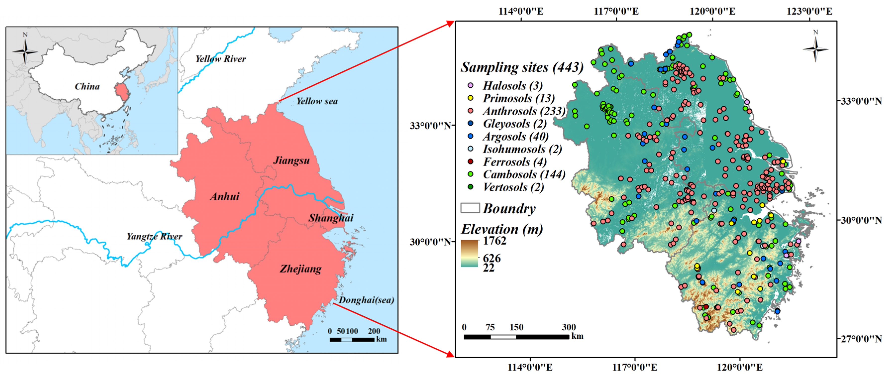
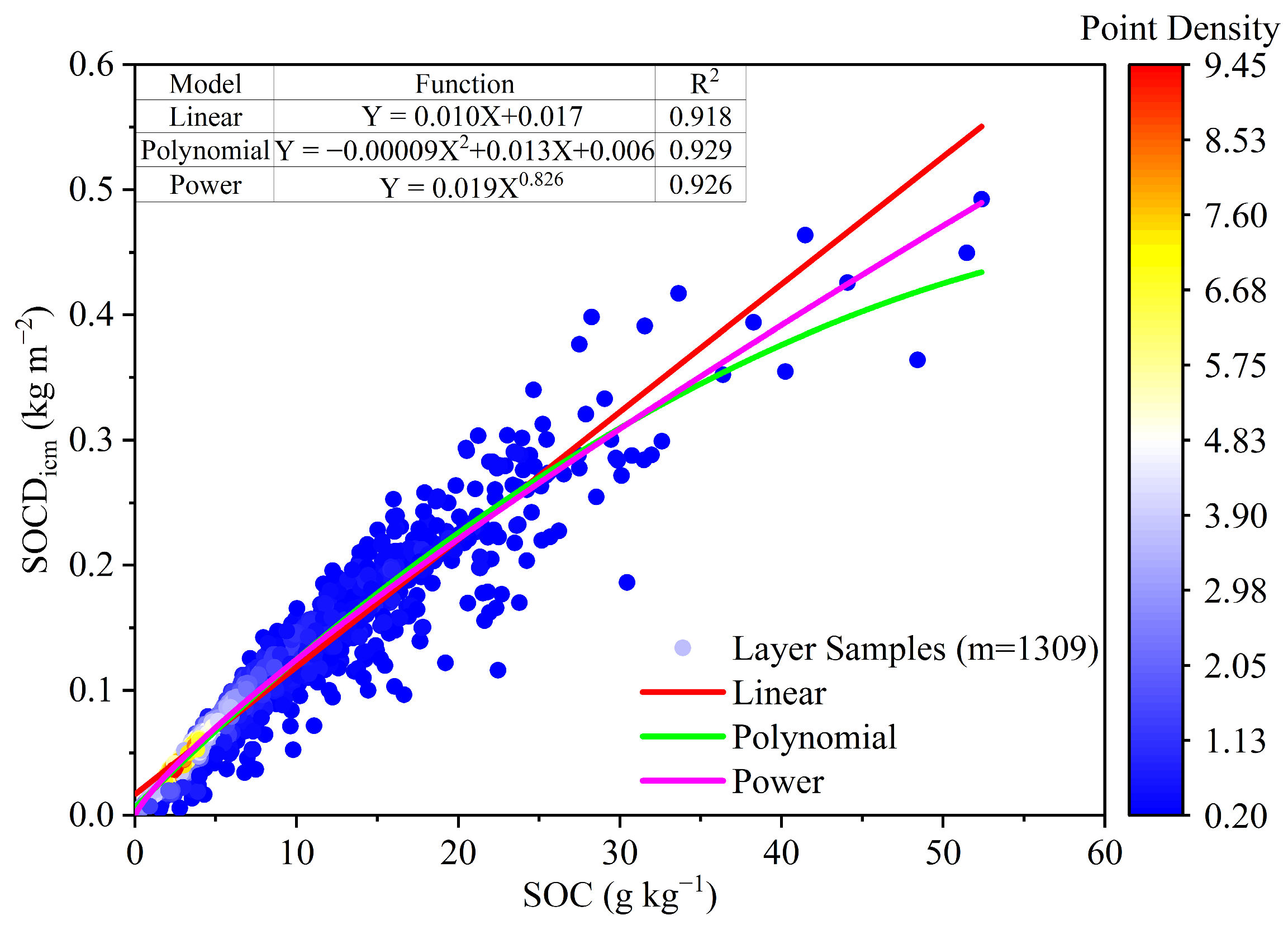
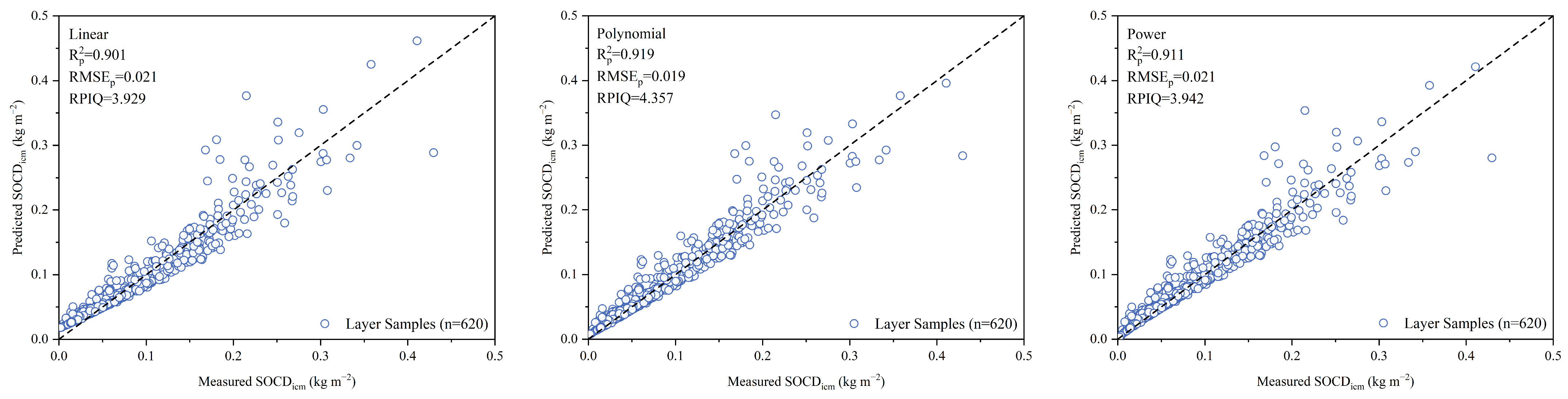
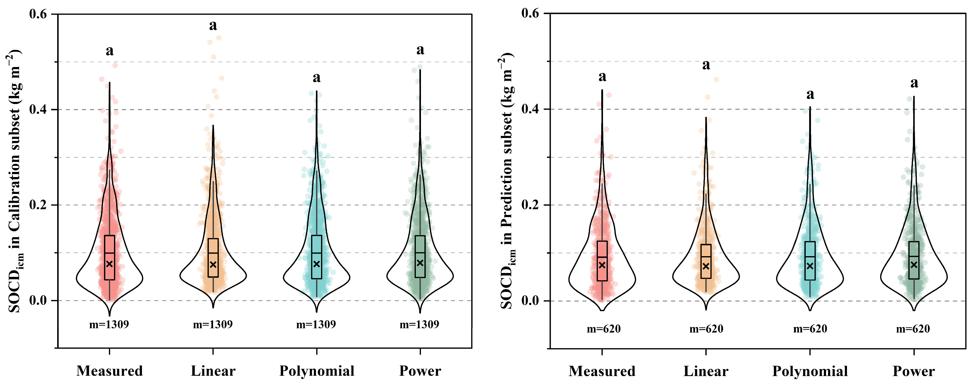
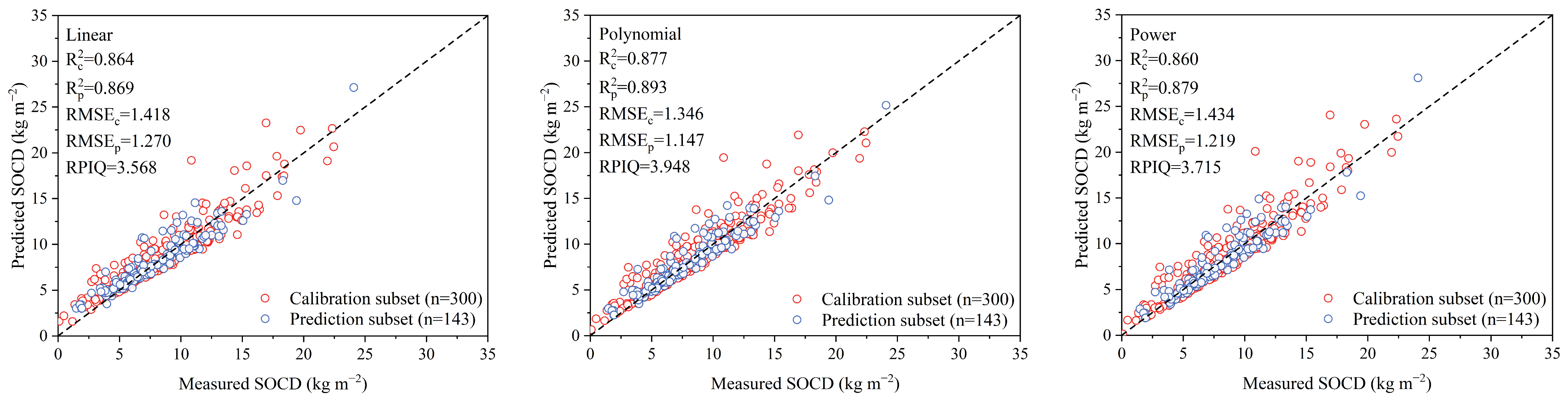
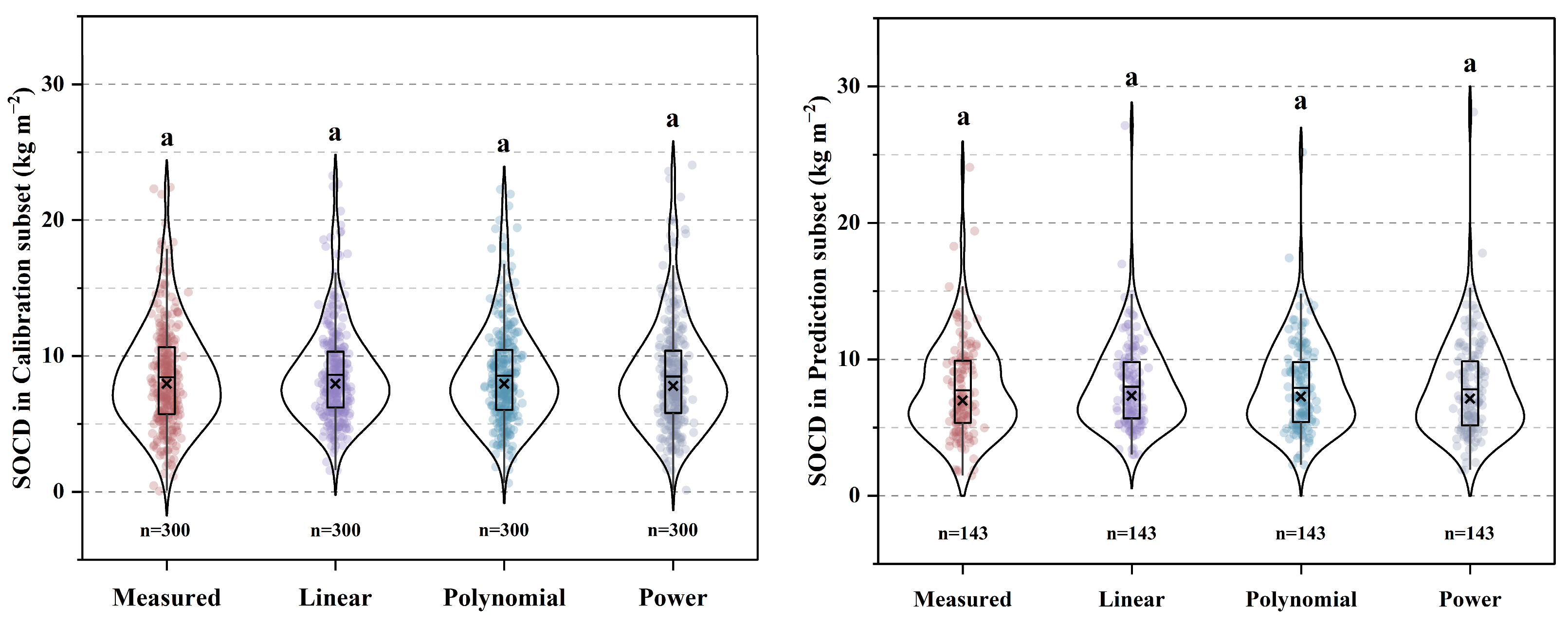
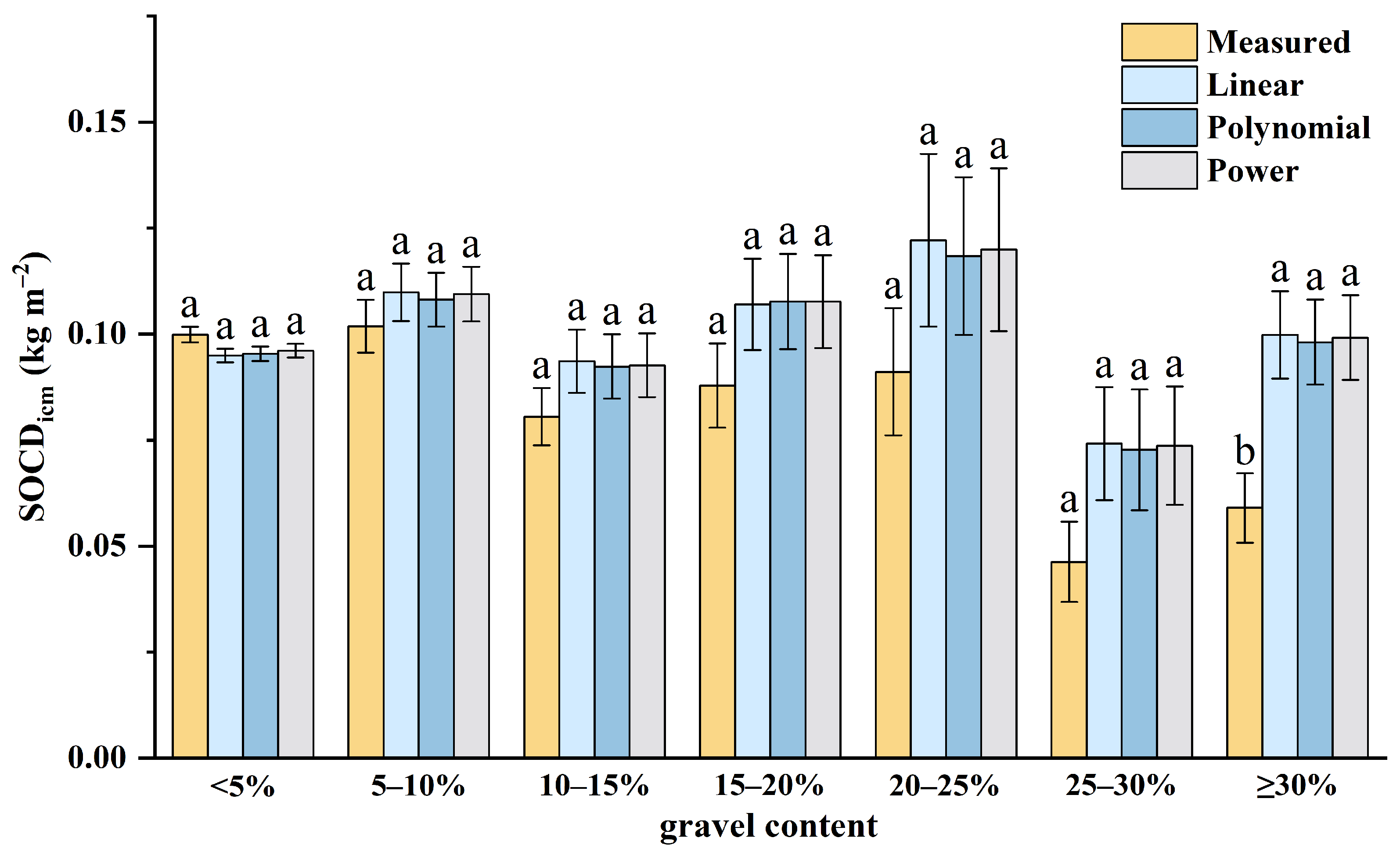
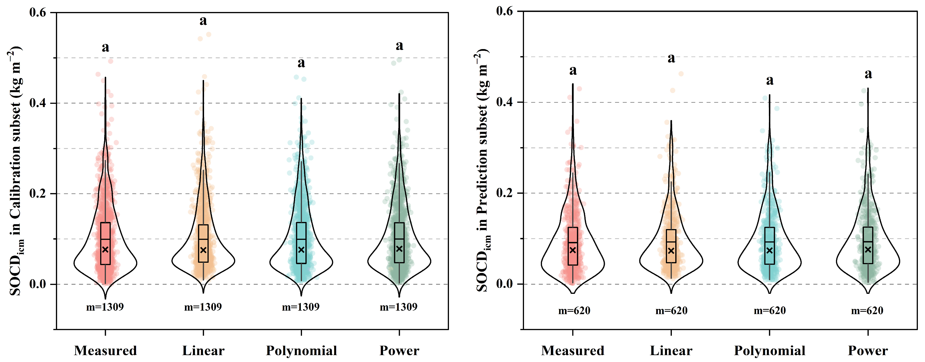
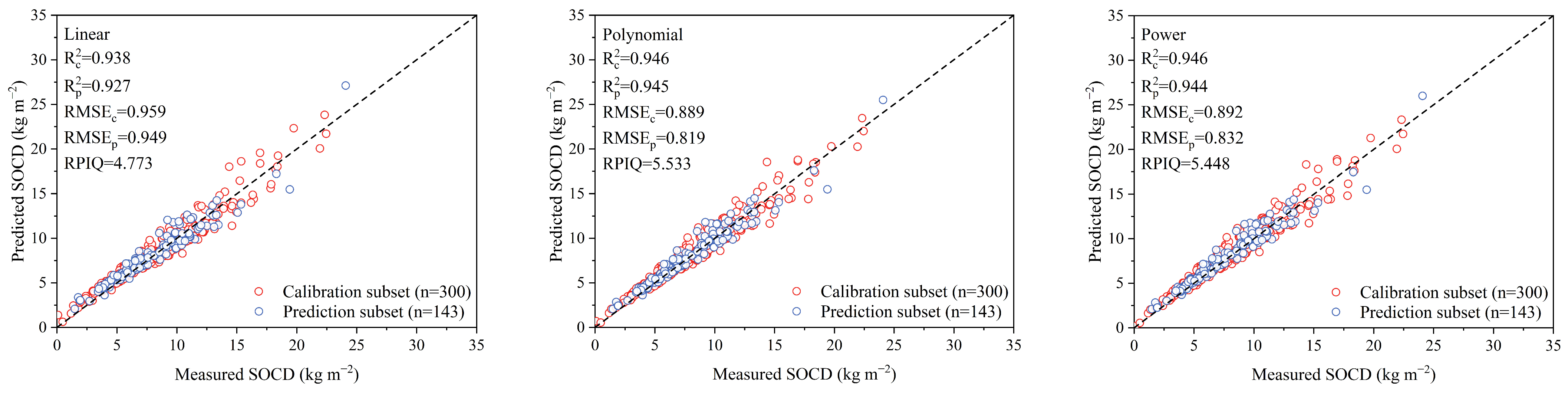
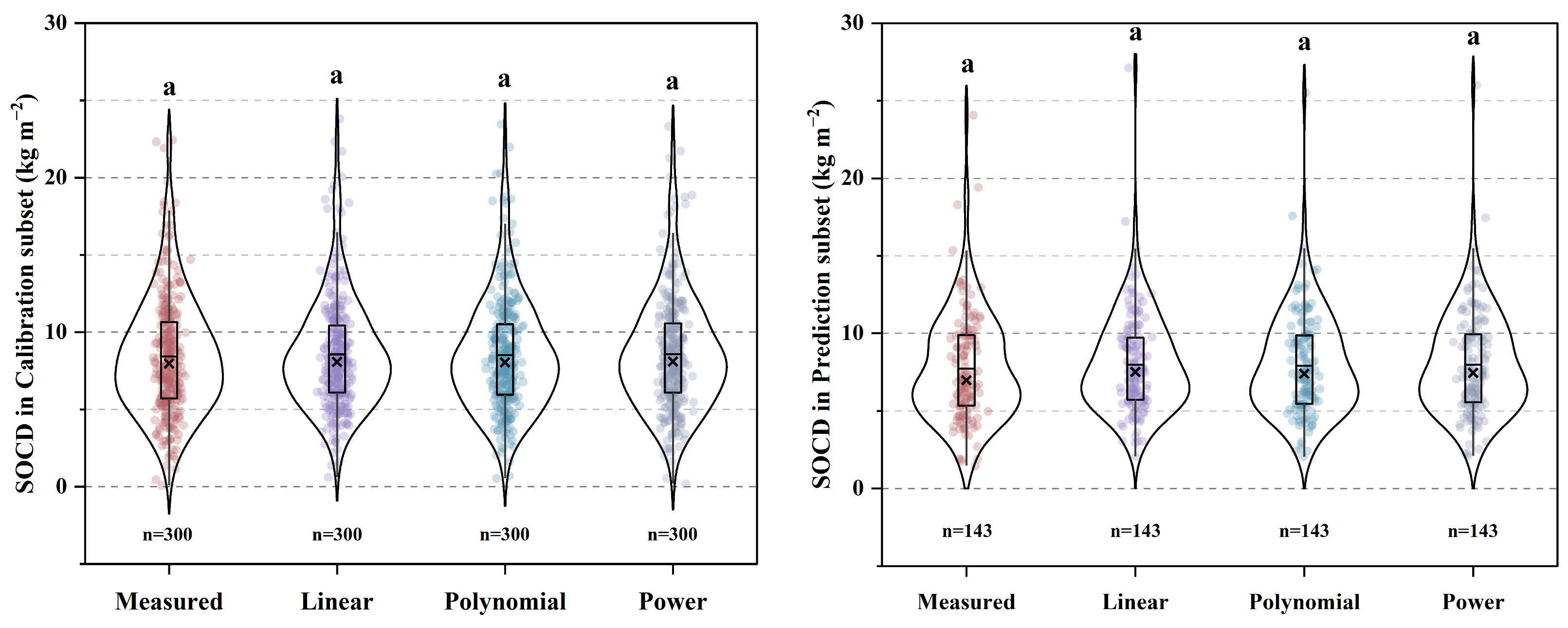
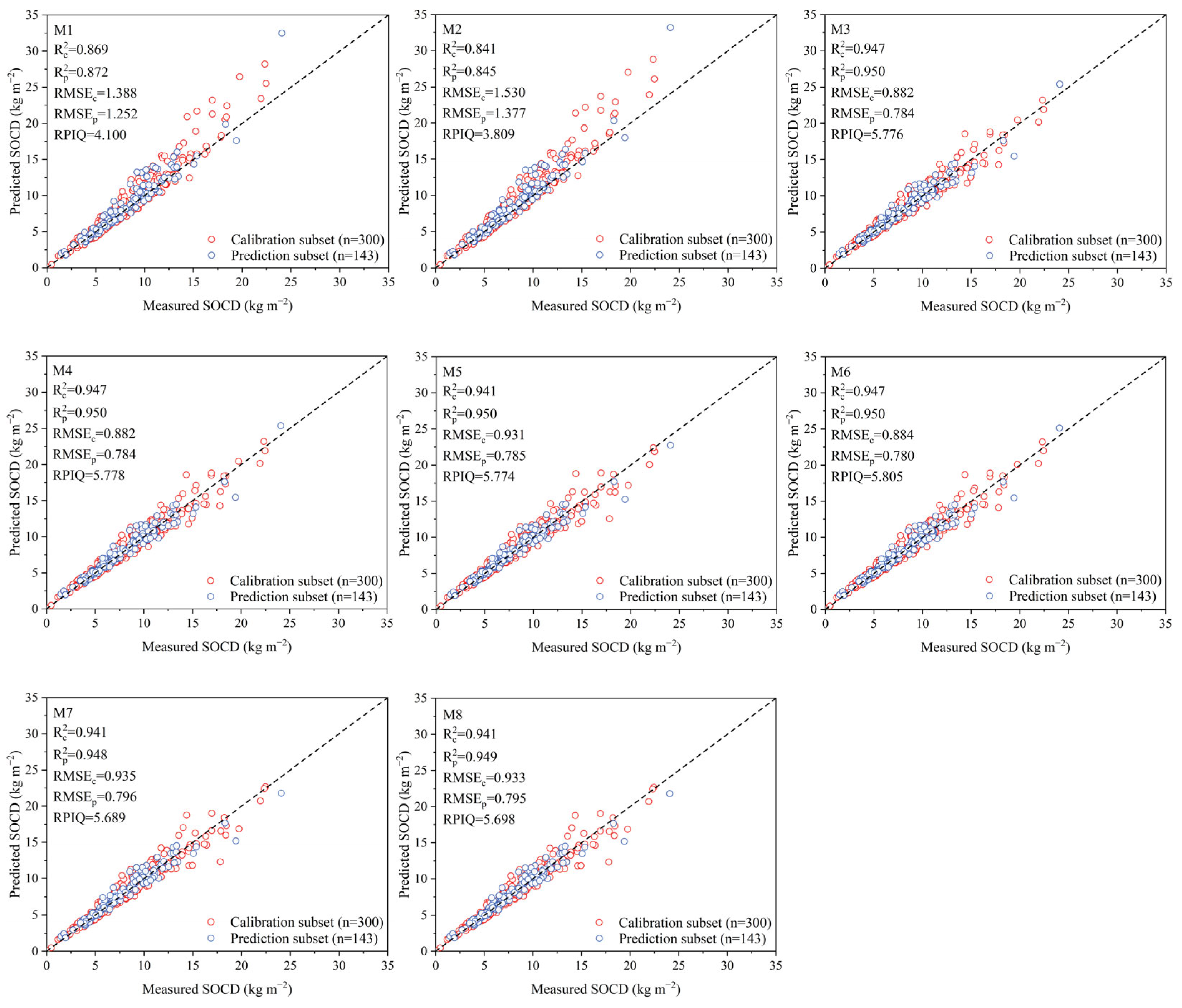

Disclaimer/Publisher’s Note: The statements, opinions and data contained in all publications are solely those of the individual author(s) and contributor(s) and not of MDPI and/or the editor(s). MDPI and/or the editor(s) disclaim responsibility for any injury to people or property resulting from any ideas, methods, instructions or products referred to in the content. |
© 2025 by the authors. Licensee MDPI, Basel, Switzerland. This article is an open access article distributed under the terms and conditions of the Creative Commons Attribution (CC BY) license (https://creativecommons.org/licenses/by/4.0/).