Abstract
Global warming poses significant threats to agriculture, ecosystems, and human survival. This study focuses on the arid inland Manas River Basin in northwestern China, utilizing nine CMIP6 climate models and five multi-model ensemble methods (including machine learning algorithms such as random forest and support vector machines) to evaluate historical temperature and precipitation simulations (1979–2014) after bias correction via Quantile Mapping (QM). Future climate trends (2015–2100) under three Shared Socioeconomic Pathways (SSP1-2.6, SSP2-4.5, and SSP5-8.5) are projected and analyzed for spatiotemporal evolution. The results indicate that the weighted set method (WSM) significantly improves simulation accuracy after excluding poorly performing models. Under SSP1-2.6, the long-term average increases in maximum temperature, minimum temperature, and precipitation are 1.654 °C, 1.657 °C, and 34.137 mm, respectively, with minimal climate variability. In contrast, SSP5-8.5 exhibits the most pronounced warming, with increases reaching 4.485 °C, 4.728 °C, and 60.035 mm, respectively. Notably, the minimum temperature rise gradually surpasses the maximum temperature, indicating a shift toward warmer and more humid conditions in the basin. Spatially, high warming rates are concentrated in low-altitude desert areas, while the precipitation increases correlate with elevation. These findings provide critical insights for climate adaptation strategies, sustainable water resource management, and ecological conservation in China’s arid inland river basins under future climate change.
1. Introduction
In August 2021, the Intergovernmental Panel on Climate Change (IPCC) Sixth Assessment report “Climate Change 2021: The Basis of Natural Science” pointed out that the global warming trend will continue until at least the middle of this century, and many changes in the climate system will be intensified to varying degrees with regional vulnerability and exposure differences, among which the inland river basin in Northwest China is a high-risk area for high temperature and drought [1]. The Manas River Basin, as a typical inland arid river basin in Northwest China, is located in the central area of the economic belt on the northern slope of the Tianshan Mountains in Xinjiang, China, and at the southern edge of the Junggar Basin. Climate change will have a more significant impact on regions where glaciers, snow, and deserts coexist, posing greater risks and challenges to the local water resources’ temporal and spatial distribution pattern, flood control, and water ecological environment protection [2].
Climate warming increases the concurrent frequency of drought and high-temperature events in the basin [3]. It simultaneously changes the distribution of regional water and heat resources, significantly affecting food production [4], human health [5], and the ecological environment [6], and will further exacerbate the future risks in these areas [7]. Therefore, assessing temperature and precipitation simulation capabilities and predicting future climate change are important for water resources management and decision-making. In order to mitigate and cope with climate change, since the Coupled Model Intercomparison Project (CMIP) in 1995, major climate modeling centers around the world have released a large amount of climate model data [8]. This has now reached CMIP6, which is the latest stage with the largest number of models involved, the most complete design experiments, and the most data provided—the primary subplan of CMIP6 is ScenarioMIP [9]. The CMIP6 scenario uses a new framework combining Shared Socioeconomic Pathway and Representative Concentration Pathways [10]. It reflects the relationship between radiative forcing and social and economic development and can be adapted to the needs of different research fields [11].
To mitigate the inherent uncertainties of individual CMIP6 models, multi-model ensemble (MME) approaches have emerged as a cornerstone in climate prediction. These methods broadly fall into two categories: the simple composite method (SCM), which averages outputs across models, and the weighted set method (WSM), which assigns performance-based weights to individual models [12]. Empirical studies demonstrate that both SCM and WSM consistently outperform single-model projections across diverse evaluation metrics, including spatial correlation and error reduction [13]. However, with the development of climate models, MME faces two major challenges. First, MME simulations are more sensitive to model simulations, and directly using all models will reduce the simulation capacity of MME, so it is necessary to eliminate poor performing models before actual use [14]. Second, the number of global circulation models (GCMs) proposed by different institutions is increasing, but most have structural similarities, such as model resolution, physical parameterization, and even entire atmospheric or oceanic components [15]. This lack of independence among models complicates the application of linear weighting schemes, potentially obscuring robust climate signals. Recent advances in machine learning offer promising avenues to address these challenges by enabling nonlinear ensemble optimization and automated model selection, as explored in later sections.
In the last decade, machine learning methods have received increasing attention from different disciplines for their excellent results in classification and regression problems [16]. In addition, a number of nonlinear estimators based primarily on machine learning have been used in MME and, in most cases, have demonstrated an improved evaluation performance compared to traditional methods. For example, Wang, et al. [17] applied four MME methods—including two machine learning methods, random forest (RF) and support vector machine (SVM)—to reproduce the monthly rainfall and temperature in Australia and found that the machine learning method was superior to the traditional MME and all members. Crawford, et al. [18] used RF, artificial neural network (ANN), multiple linear regression, and weighted K-nearest neighbor (KNN) to forecast monthly temperature and precipitation in parts of North America and showed that RF performed the best. Ahmed, et al. [19] evaluated different machine learning methods [ANN, KNN, SVM, and correlation vector machine (RVM)] in the MME prediction of precipitation and temperature in Pakistan and concluded that KNN and RVM were superior.
In recent years, machine learning algorithms have gained prominence in climate science for their ability to capture complex, nonlinear relationships within high-dimensional datasets. Among the widely adopted techniques, RF excels in handling feature interactions and mitigating overfitting through ensemble decision trees, though its “black-box” nature limits interpretability [17]. SVM, leveraging kernel-based transformations, demonstrates robustness in small-sample scenarios but faces computational bottlenecks with large-scale data [18]. ANN offers unparalleled flexibility in modeling spatiotemporal patterns yet requires extensive training data and computational resources [19]. While these methods have individually advanced climate projections—from extreme temperature prediction [20] to precipitation downscaling [21]—their standalone applications often struggle with inherent limitations: RF may overlook subtle temporal dependencies, SVM lacks the scalability for multi-decadal simulations, and ANN risks overfitting under sparse observational constraints.
To transcend these constraints, MME approaches have emerged as a pivotal strategy, synthesizing diverse ML frameworks to offset individual biases and enhance predictive stability. However, conventional MME methods, such as SCM or WSM, remain challenged by structural redundancies among climate models and nonlinear error propagation [22]. This study addresses these gaps by integrating ML-driven weighting with CMIP6 multi-model data, optimizing the ensemble performance for arid inland basins.
At present, research on predicting regional climate change in China using the CMIP6 model is gradually being carried out. However, no scholars have combined RF, ANN, SVM, and other machine learning methods to assess precipitation and temperature in the Manas River Basin. Under the influence of different social and economic development and greenhouse gas emissions, the change trends in temperature and precipitation in the basin were studied. Using the HRLT dataset as observational data, this paper evaluates the downscaling and bias-corrected CMIP6 GCM, takes the Manas River Basin as an example, evaluates the simulation ability of temperature and precipitation, and predicts the changes in temperature and precipitation in the basin from 2021 to 2100 using the newly proposed SSP scenarios. This will provide ideas and references for coping with climate change in China’s arid inland river basins.
2. Data and Methods
2.1. An Overview of the Study Area
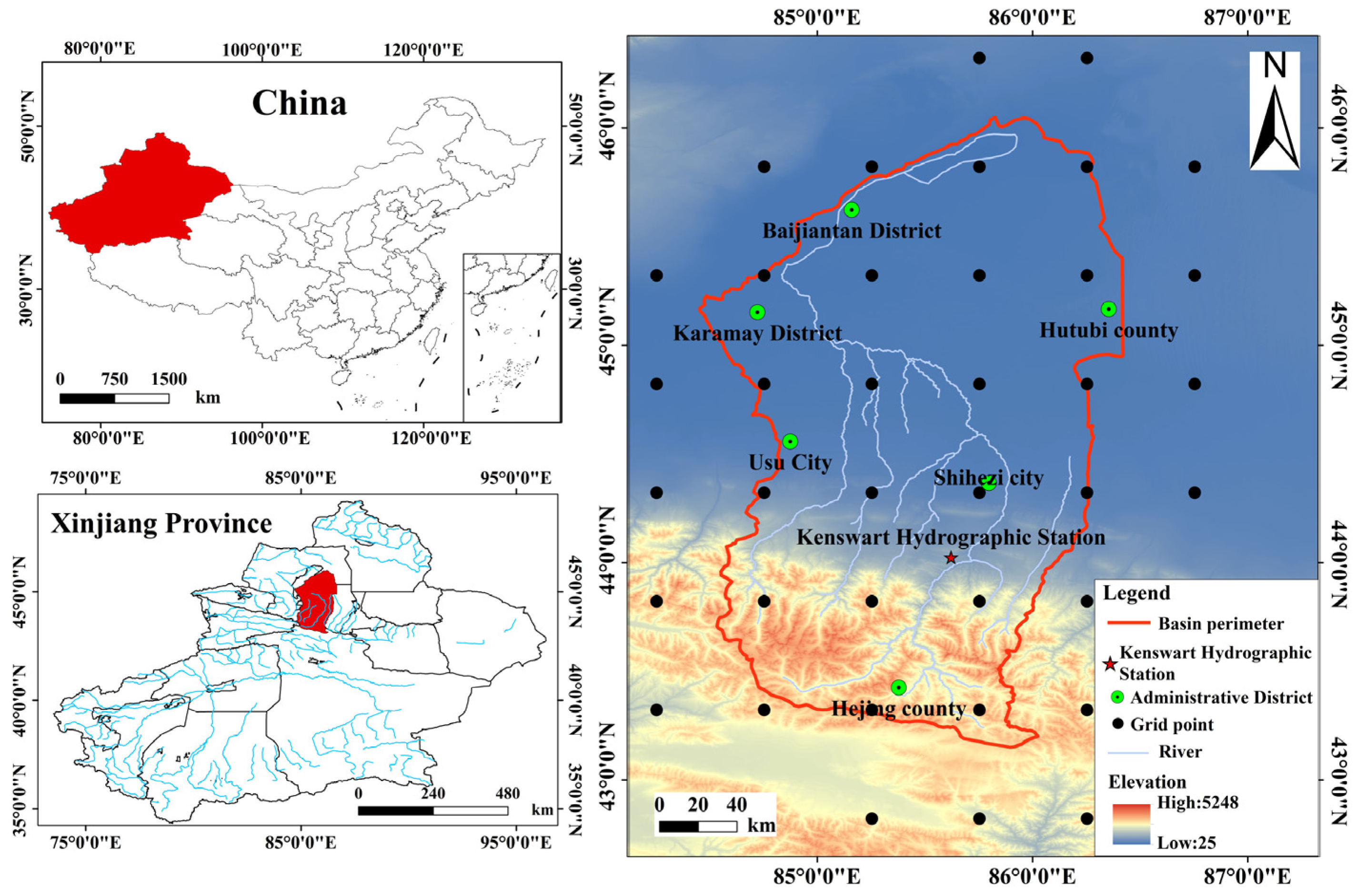
The Manas River Basin, the core area of the Xinjiang Economic Development Zone in Northwest China, is located in the southern margin of the Junggar Basin. Located at 84°44′–86°50′ E, 43°4′–46°0′ N, the landforms in succession from south to north are mountains, then plains, and then deserts. The overall terrain is high in the south and low in the north, with the highest elevation reaching 5246 m. The total basin area of the study area is about 2.67 × 10⁴ km2 (Figure 1). The Manas River Basin is far from the ocean and has a typical temperate continental arid climate [23]. The temperature difference between day and night in winter and summer is large. The extreme maximum temperature in summer is 43.1 °C, the extreme minimum temperature in winter is −42.8 °C, and the average annual temperature is 5.0–7.5 °C. The annual distribution of precipitation is uneven; there is more in spring and summer than in autumn and winter, with about 70% in the rainy season of June–September [24].
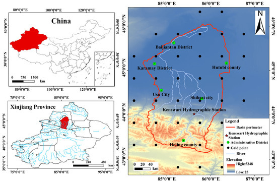
Figure 1.
A location map of the research area.
2.2. Data Sources
2.2.1. HRLT
The research data in this paper were mainly divided into observation data and simulation data (Table 1). The observational data were obtained from the daily gridded China maximum temperature, minimum temperature, and precipitation HRLT dataset [25]. The daily grid data were interpolated using comprehensive statistical analysis, including machine learning, generalized additive models, and thin plate splines. The model was based on the 0.5° × 0.5° raster dataset of the China Meteorological Administration, and the accuracy of the HRLT daily dataset was evaluated using the observation data from weather stations. The results show that the precision of HRLT is higher than that of CMFD [26,27], the China Meteorological Administration Land Data Assimilation System (CLDAS, https://data.cma.cn/ (Accessed on 10 October 2024)), and the Inter-Sectoral Impact Model Intercomparison Project (ISIMIP3a, https://data.isimip.org/ (Accessed on 10 October 2024)). A detailed data description is provided in Text S1, Table S1.

Table 1.
Details of observed data.
2.2.2. GCM Data
This paper forecasts meteorological data mainly related to the daily maximum and minimum temperature and daily precipitation data from CMIP6 (https://esgf-index1.ceda.ac.uk/projects/cmip6-ceda/ (Accessed on 10 October 2024)). Nine global climate models were selected to evaluate the ability of the CMIP6 global climate model to simulate temperature and precipitation in the study area (Table 2). Based on the years that can be simulated in the historical period of the climate model and the farthest years that can be predicted in the future scenario, the period 1979–2014 was taken as the base period of historical climate simulation evaluation, and the chosen future period was 2015–2100. This paper selects three future scenarios in CMIP6 (Table 1): climate elements under SSP1-2.6, SSP2-4.5, and SSP5-8.5. The Scenario Model Comparison program used a new matrix combination of SSPs and RCPs to describe the possible future development of society without the impact of climate change or climate policies, with greater emphasis on the consistency of future radiative forcing scenarios with shared socioeconomic scenarios [28]. A detailed data description is provided in Text S1, Table S2.
Table 2.
Climate model information.
2.3. Research Method
2.3.1. Downscaling and Bias Correction
There are differences in the spatial resolution of data from different climate models. To more accurately compare CMIP6 model data with observational data and better adapt to regional scale climate research, we first used a bilinear interpolation method for CMIP6 model data [29] and carried out spatial scaling and unified interpolation on a grid with a spatial resolution of 0.5° × 0.5° for analysis and research.
Since there are systematic errors in the simulation of precipitation and temperature in climate models, the QM method [30] was used in this paper to correct the errors. Numerous scholars’ research indicates that QM can effectively correct model data and reduce errors [31,32]. QM is a correction method based on frequency distribution, and the QM method assumes that the frequency distribution between the observed data and simulated data is consistent. The method first constructs a transfer function between the cumulative probability distribution function of the historical observations and the simulated values and then corrects the simulated values in the future period [33]. The QM was constructed as follows:
where xm,h represents the result of bias correction; Fobs and Fm represent the cumulative distribution functions of the observational data and model data in the historical period, respectively; and xm,fut represents the raw data of mode m during the prediction period.
2.3.2. MME Method
Due to the systematic bias and the uncertainty of the initial field of the numerical model itself, a single “optimal” model has a large deviation, which often has a great effect on the impact assessment of climate change. Comparing a single numerical model to a multi-model ensemble forecast is an effective way to improve the model accuracy [34].
- SCM and WSM
The formulas for SCM and WSM are shown as Equations (2) and (3):
where TSCM and TWSM represent the simple, complex, and weighted set methods based on the correlation coefficient, respectively. Fx is the simulation result of the single model. is the weight of a single model based on the correlation coefficient r, and rx is the weight of a single model based on r.
- 2.
- RF
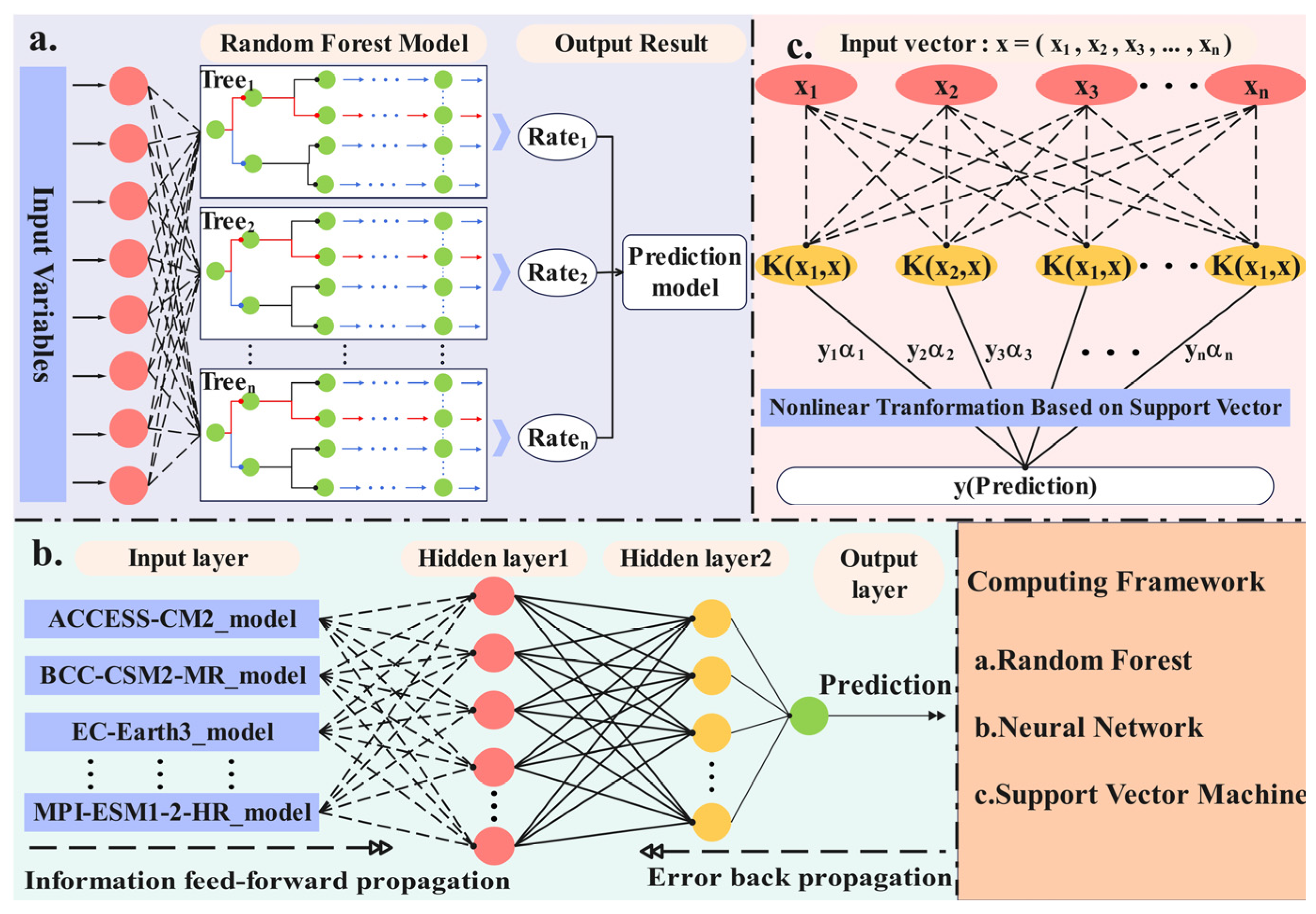
The RF is a combinatorial classifier containing multiple decision trees for nonlinear relationships between the predicted and reference values [35]. The combinational classifier introduces an independent and equally distributed random variable θ and uses the training dataset and θ to generate decision trees . Finally, ensemble learning is used to combine all decision trees. The algorithm takes the mean of the predicted values of each decision tree (Figure 2a). According to existing CMIP6 models, the corresponding sequence values are predicted by inputting them into the RF model. The final simulation result is the average of all trees to simulate the whole. The detailed description and parameter settings of the RF model are presented in Text S2.
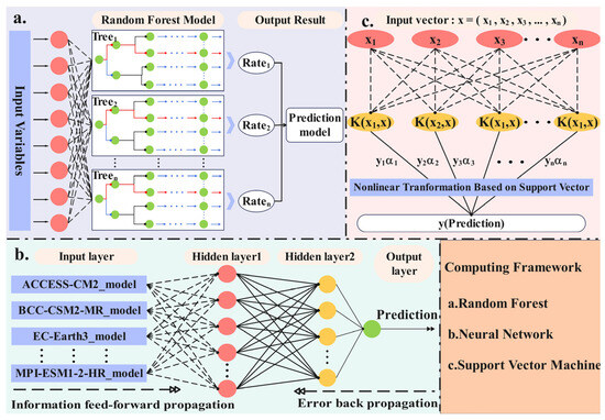
Figure 2.
Machine learning model framework.
- 3.
- ANN
Neural networks are computational tools for tasks such as classification, regression, and clustering [36]. Inspired by biological research on brain structure, these systems simulate brain-like information processing through interconnected nodes (neurons). Each neuron exchanges signals with others, and the network collectively processes data through layered connections (Figure 2b). When trained on datasets like CMIP6 model outputs, neural networks autonomously identify patterns to generate predictions. The detailed description and parameter settings of the ANN model are presented in Text S3.
where y_ANN(t) is the forecast value at time t of model output. f is the transfer function, and this article uses the relu function: f(x) = max(0,x_ANN). ωj is the weight coefficient connecting the hidden layer and the output layer. xi_ANN(t) is the value of the ith climate factor at the input time of the model. υij is the weight coefficient of the connecting layer and the hidden layer. n is the number of climate factors. m is the dimension of the hidden layer. θj is the threshold of the hidden layer, and θ0 indicates the threshold of the output layer.
- 4.
- SVM
Support vector machine (SVM) is a supervised learning algorithm developed by Vapnik and Chervonenkis for classification, regression, and outlier detection [37]. SVM excels in handling nonlinear data by mapping linearly inseparable samples into a high-dimensional feature space via kernel functions. This mapping allows the identification of an optimal hyperplane that maximizes the separation between classes, transforming the problem into a convex quadratic optimization task. For nonlinear regression, SVM similarly leverages kernel-based transformations (Figure 2c). Detailed parameter configurations are provided in Text S4. Suppose that the sample dataset , where x is the vector of the input variable and y is the output value, follows a linear regression model:
where ⟨ ⟩ is the dot product, w is the unit normal vector of the hyperplane, and b is the distance from the origin to the hyperplane. For tolerance margin ε, an optimal function Le is proposed to determine the optimal hyperplane:
This problem can be translated into its Lagrange duality formula after a series of calculations, expressed as follows:
where αi and are Lagrange multipliers and K is a kernel function. In this study, the radial basis function was chosen to follow the kernel model of previous studies.
2.3.3. Cross-Validation and Skill Metrics
To evaluate the simulation capability of each model and further select the model for future scenario prediction, this paper uses the Taylor diagram, Taylor skill score (TSS) [38], spatial skills score (SS) [39], interannual variability skill score (IVS) [40], Kling–Gupta efficiency (KGE) coefficient [41], and four other evaluation indicators. Finally, according to the evaluation results of each single index, a comprehensive ranking of the simulation capabilities of each model was provided using the comprehensive ranking index (CRI) [42]: Equations (9)–(18).
- Taylor diagram and TSS
The Taylor diagram, developed by Karl E. Taylor [43], is a tool widely adopted by the IPCC to assess model performance. It visually compares simulations against observations using three metrics: standard deviation (STD), root mean square error (RMSE), and correlation coefficient (r). Radial distances from the origin represent STD ratios relative to observations, while distances between the model and reference points indicate RMSE (smaller values imply better accuracy). The angular position reflects the correlation strength (higher r values correspond to smaller angles). In this study, the diagram evaluates the CMIP6 models’ precipitation and temperature simulations, aiding in selecting optimal models for regional hydrological forecasts [44].
The TSS is a numerical generalization of the Taylor diagram, a composite indicator of its predictive skill, and is often used as a composite measure to evaluate different GCM and post-processing techniques [45]. The range of TSS values is 0–1, with values closer to 1 indicating better simulation by the model. The formula for calculating TSS is Equation (9):
where R is the spatial correlation coefficient between simulation and observation, R0 is the maximum attainable correlation coefficient (set to 0.999) [46], and σsm and σso are the STDs of the climate mean for simulated and observed spatial models, respectively.
- 2.
- SS
Let Mk and Ok be the precipitation model data and the observation data, respectively. Then, the spatial field square error of observation and evaluation is defined as follows:
where N is the number of space lattice points. Taking into account the dimensionlessness of the above equation, the dimensionless SS is obtained:
where rm,o is the spatial correlation coefficient between the model data and observation data; Sm and So are the STDs of the model and observation, respectively; and and ō are the regional averages of the evaluation and observation fields, respectively. This score takes into account the degree of spatial correlation and deviation between the model data and the observed data. The larger the correlation coefficient and the smaller the deviation value between the model data and the observed data, the closer the score value is to 1, indicating higher spatial accuracy of the model data [47].
- 3.
- IVS
The IVS is used to assess the performance of capturing interannual variation and is expressed as follows:
where σtm and σto represent the STD of the interannual variation in the simulation data and the observation data, respectively. Smaller IVS values indicate better performance.
- 4.
- KGE
The KGE is a model parameter calibration method proposed by Kling and Gupta et al. in 2009, which fully considers the mean and variance of the model data and the measured data [48]. It is a comprehensive index combining the correlation coefficient, mean error, and standard error. The value range of KGE is (−∞, 1); the closer it is to 1, the better the simulation. The KGE is calculated using Equations (14)–(17):
- 5.
- CRI
When evaluating the simulation ability of different models on observed data, a single index will produce different evaluation results. Therefore, the CRI was introduced, which provides a comprehensive ranking of the simulation capability of each model according to the evaluation results of each single index [49]. The CRI is calculated using Equation (18):
where m is the number of models considered in the evaluation, n is the number of individual evaluation indicators, and Ranki is the rank of the model in each evaluation indicator. The CRI ranges from 0 to 1, with values closer to 1 indicating better model performance.
3. Results and Discussion
3.1. Model Simulation Ability Evaluation
3.1.1. Taylor Diagram and Linear Trend Analysis
QM bias correction significantly improved the model simulations, as evidenced by the increased r, reduced MAE, and reduced RMSE in the corrected outputs (Figure S1 and Table S6). Overall error metrics were notably enhanced, as detailed in Text S5. Based on the HRLT dataset, a Taylor diagram was constructed to evaluate the spatiotemporal simulation capabilities of nine CMIP6 models and five MME methods for precipitation, maximum temperature, and minimum temperature in the Manas River Basin. Climate models with poor performance—characterized by low prediction accuracy, elevated deviations, and heightened uncertainty—were identified to avoid misleading decision-making. Consequently, four models demonstrating the weakest simulation results (correlation coefficients < 0.97 for temperature variables and <0.50 for precipitation) were excluded. This elimination process refined the MME framework, yielding superior simulation performance (Table S7).
- Taylor diagram and trend analysis of temperature
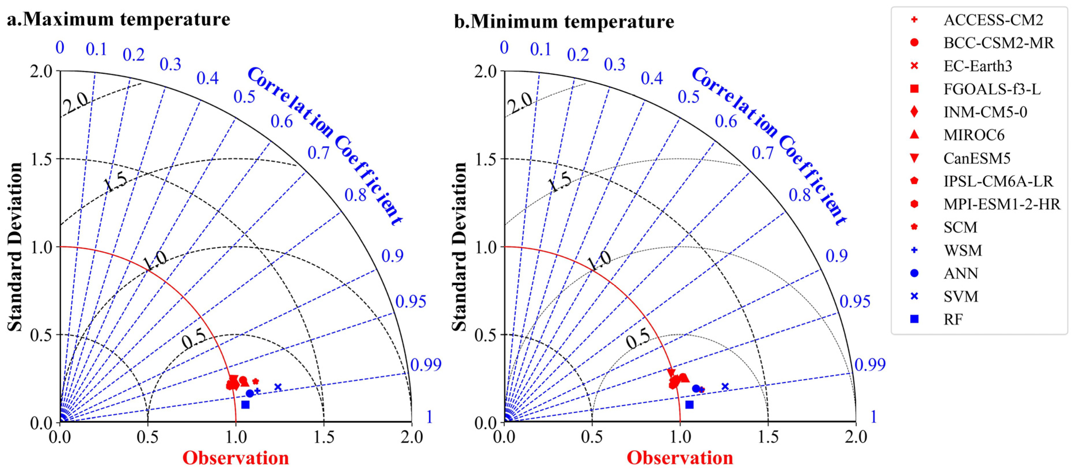
The Taylor diagram was used to measure the simulation results of climate models on the temperature of the Manas River Basin (Figure 3). The simulation differences between the maximum and minimum temperatures of different climate models were not obvious, and the correlations with observed values were highly consistent. The mean maximum temperature for historical observations was 10.57 °C. For the model, it was 10.54–10.56 °C, and for the SCM, it was 10.56–10.82 °C. The simulated RF value was the closest to the observed value, with an r of 0.995, an RMSE value of 0.037 (the lowest among all the models), and an STD of 1.06. The correlations of other models exceeded 0.97, RMSEs were below 0.1, and STDs were within ±0.1 except for SVM.
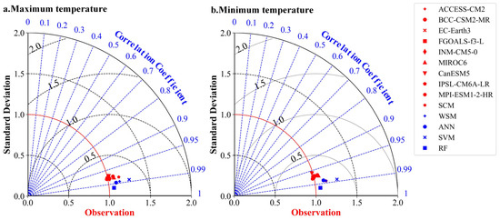
Figure 3.
A simulated Taylor diagram of monthly mean temperature in the Manas River Basin for 1979–2014.
The mean of the minimum temperature observed in the historical period was −1.40 °C. For the model, it was −1.40 to −1.42 °C, and for the SCM, it was −1.19 to −1.41 °C. The simulated value of RF was the closest to the observed value, with an r of 0.995, an RMSE of 0.038 (the lowest among all the models), and an STD of 1.06. The correlations for other modes exceeded 0.96, the RMSE was below 0.1, and the STD was within ±0.1 except for SVM.
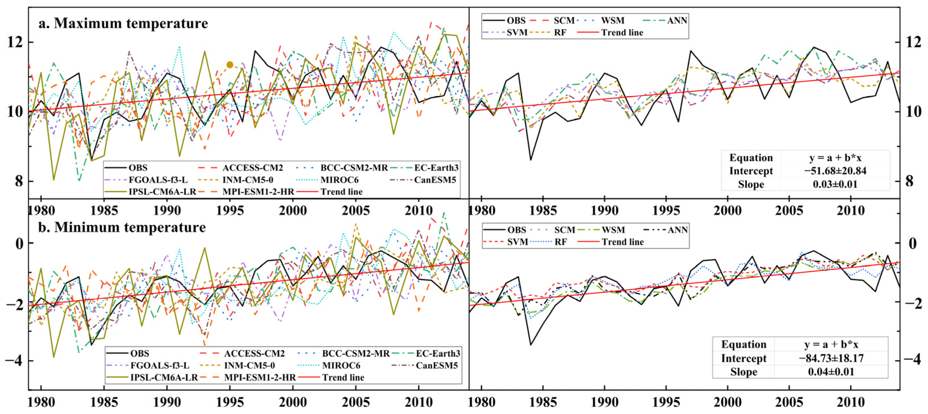
To further analyze the trend characteristics of the temperature simulation results, a linear trend was used for fitting analysis (Figure 4). The observed maximum temperature (slope 0.032) and minimum temperature (slope 0.042) in the historical period showed a significant increasing trend. The maximum temperature increased from 9.83 °C in 1979 to 10.24 °C in 2014, with an average increase rate of 0.012 °C/a. The minimum temperature increased from −2.36 °C in 1979 to −1.52 °C in 2014, with an average increase rate of 0.024 °C/a. All model data values showed a fluctuating change around the center line, among which the MPI-ESM1-2-HR model was the closest to the observed value. In the simulation of minimum temperature, there were large deviations in individual years, mainly in 1984 and 1997, at 1.83 and 1.49 °C lower than the observed values, respectively. The CanESM5 model was repeatedly inconsistent with the observed values in multiple years, mainly for the maximum temperature—namely in 1983, 1999, 2008, 2010, and 2014—consistent with the results in Figure 3. The SCM data and observed data maintained a high consistency in the trend of change, but the overall curve fluctuation was small, indicating a large deviation when the climate changed. For example, in 1984, the observed temperature suddenly dropped, but the SCM did not reach a corresponding extreme value, which also indicates that the ability of each model to simulate the extreme change in climate was somewhat insufficient. The CanESM5, IPSL-CM6A-LR, BCC-CSM2-MR, and SVM poorly simulated the maximum and minimum temperature and so were excluded.
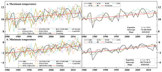
Figure 4.
Annual temperature changes in the Manas River Basin during the period of 1979–2014.
- 2.
- Taylor diagram and trend analysis of precipitation
Compared with the simulation of temperature, the simulations of precipitation of each model were not ideal (Figure 5), and the correlation coefficients were −0.22 to 0.944, indicating that the same models had different simulations of temperature and precipitation and should be analyzed separately. The average precipitation observed in the historical period was 270.46 mm. In the model, it was 263.10–265.22 mm, and in SCM, it was 235.94–270.51 mm. Among them, RF was still the closest to the observed value, with r, RMSE, and STD values of 0.944, 0.083, and 1.05, respectively, and an average precipitation of 267.35 mm. Both MPI-ESM1-2-HR and FGOALS-f3-L were negatively correlated with the observation series, with r values of −0.22 and −0.03, respectively, showing the opposite trend compared with the observation series. Therefore, they should be eliminated.
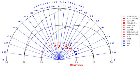
Figure 5.
A simulated Taylor diagram of monthly precipitation average in the Manas River Basin for 1979–2014.
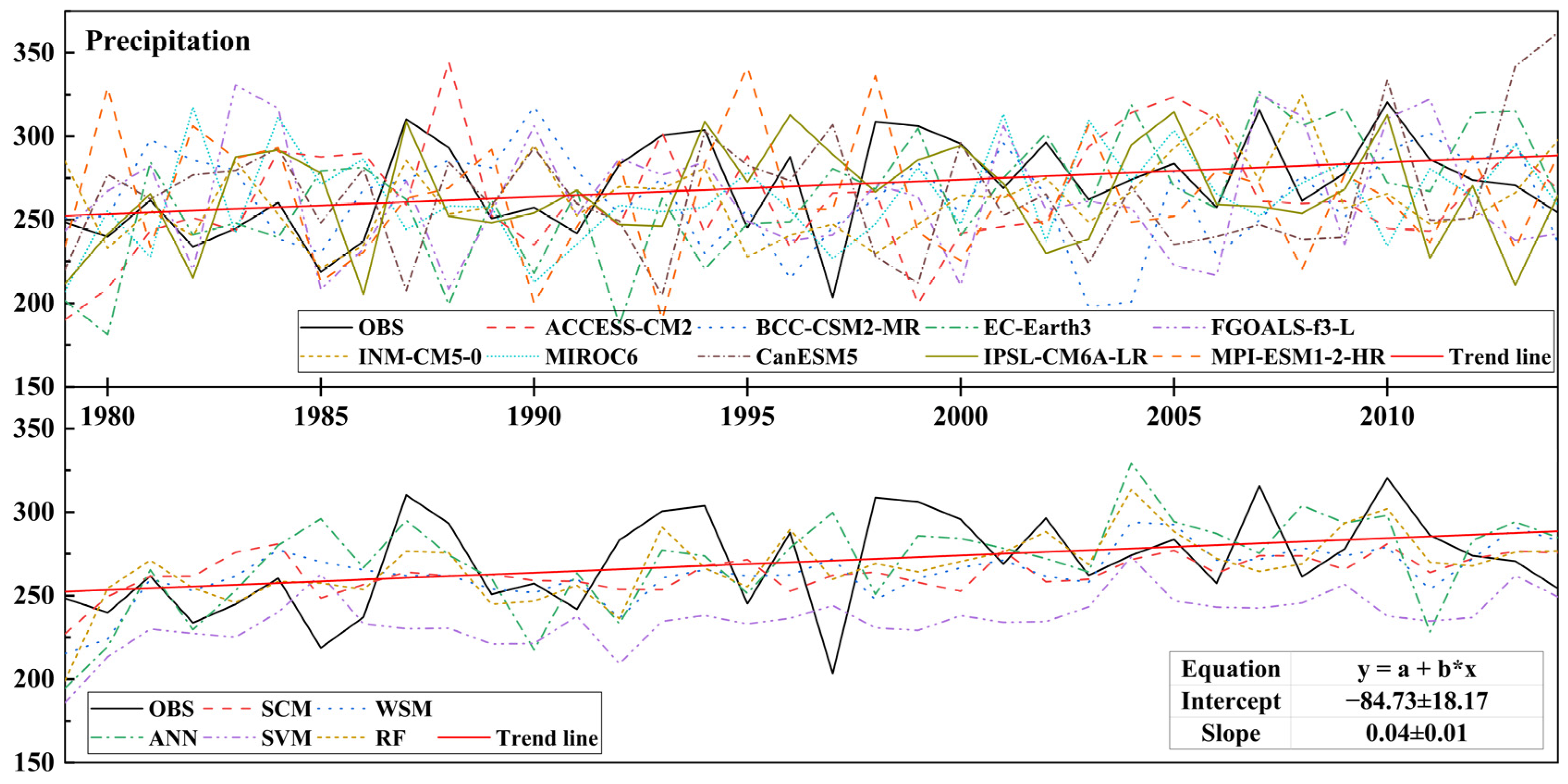
The trend characteristics of the precipitation simulations were further analyzed (Figure 6) and combined with the linear trend equation of the observed precipitation time series Y = 1.0334X + 251.34, the slope of which is 1.0334 > 1, showing a significant increasing trend. Precipitation increased from 248.42 mm in 1979 to 254.22 mm in 2014, with an average increase rate of 0.166 mm/a. Among all models, EC-Earth3 was closest to the observed value but with a large deviation in individual years, mainly 1988, 1992, and 1994, with values 94.01, 96.02, and 83.40 mm lower than the observed precipitation, respectively. The simulation of the MPI-ESM1-2-HR model was poor, and the variation trend of the observed series was opposite in many years, consistent with the results in Figure 5. The SCM analysis exhibited a great improvement compared with the results of the single-model analysis. Except for SVM, all models showed good consistency with the observed trend, and RF was more prominent in the precipitation simulation. In the precipitation simulation, MPI-ESM1-2-HR, FGOALS-f3-L, BCC-CSM2-MR, and SVM performed poorly and so were eliminated.
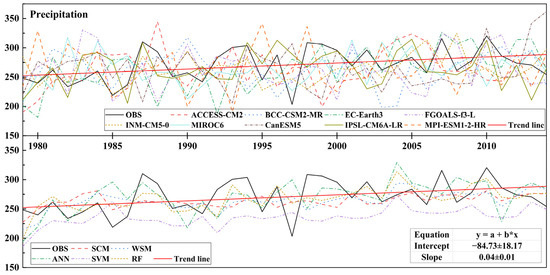
Figure 6.
Annual precipitation changes in the Manas River Basin for the period of 1979–2014.
This is because 1988 was a sudden change point in the time series of flood occurrences in Xinjiang. Since the mid-to-late 1980s, the expansion of flood losses in Xinjiang is likely to be the result of an increase in the number of heavy rainstorms and large precipitation events and the consequent increase in the frequency of floods (flood losses) within a certain time frame [50]. Around 1993, in the Manas River Basin, with an increase in the number and magnitude of floods exceeding the standard, there was also an increase in the occurrence of extreme high-temperature weather and the duration of extreme precipitation [51]. The CMIP6 models exhibit systematic deviations when simulating extreme climate events, thus causing varying degrees of deviation in individual weather phenomena, such as extreme high temperatures or extreme precipitation. These discrepancies are attributed to two primary limitations: (1) insufficient sensitivity to synoptic-scale dynamics, and (2) inadequate representation of orographically triggered convective processes during extreme rainfall events. Furthermore, coarse-resolution parameterizations fail to resolve mesoscale interactions between topography and atmospheric circulation, leading to misrepresented precipitation extremes. To address these shortcomings, future efforts should prioritize convection-permitting regional climate models and advanced ensemble techniques that integrate machine learning for bias-aware dynamical downscaling. Such approaches could enhance the physical fidelity of extreme event projections, particularly in topographically complex arid regions.
3.1.2. Quantitative Evaluation of GCM Simulation Ability
After removing the models with poor performance, each model was re-evaluated, and the regional applicability of each GCM in the Manas River Basin was quantitatively evaluated against the historical observation data. The TSS, SS, IVS, and KGE were used to rank the model simulation capability. Finally, CRI was used to create a comprehensive rating for each model (Table S8).
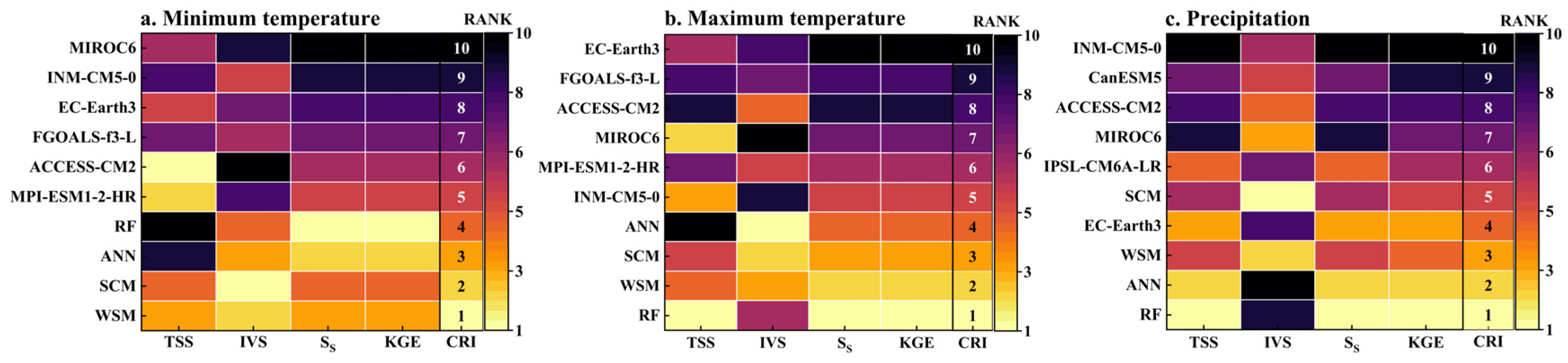
In the evaluation of regional applicability, RF, SCM, and WSM all performed better, indicating that the SCM model better simulated the temperature change in the study area after bias correction and the elimination of the models with poor performance. At a minimum temperature (Figure 7a), the best performance for TSS was ACCESS-CM2, and the worst was RF. The best performance for IVS was SCM, and the worst was ACCESS-CM2. RF was the best for SS and KGE, and MIROC6 was the worst. In the overall ranking, WSM performed the best, SCM followed, and MIROC6 performed the worst.
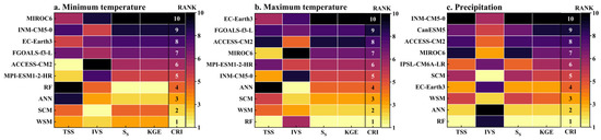
Figure 7.
GCM heat map of different evaluation indices.
For the maximum temperature (Figure 7b), RF performed the best for TSS, and ANN performed the worst. For IVS, ANN performed the best, and MIROC6 performed the worst. RF was the best for SS and KGE, and EC-Earth3 was the worst. RF was the best, WSM was second, and EC-Earth3 was the worst.
For precipitation (Figure 7c), RF performed the best for TSS, SS, and KGE, while INM-CM5-0 was the worst. SCM performed the best for IVS, and ANN performed the worst. In the overall ranking, RF was the best, followed by ANN, and INM-CM5-0 was the worst.
To sum up, after removing models with poor performance, the SCM performance improved and was better than that of a single model. As a single model, MPI-ESM1-2-HR better simulated minimum temperature, INM-CM5-0 was better at simulating maximum temperature, and EC-Earth3 was better at simulating precipitation. However, BCC-CSM2-MR and IPSL-CM6A-LR poorly simulated temperature and precipitation. After removing models with poor simulation, the WSM performance improved, and it simulated the changes in temperature and precipitation well. As RF is affected by various factors during long-term prediction, such as data quality, model selection, and feature engineering, the uncertainty of prediction is increased, and the accuracy and reliability of prediction will also decline over time. Therefore, in this paper, WSM was used to predict the future trend in the temperature and precipitation in the basin under different climate scenarios.
3.2. Spatiotemporal Changes in Temperature in Future Climate Scenarios
3.2.1. Temperature Time Variation
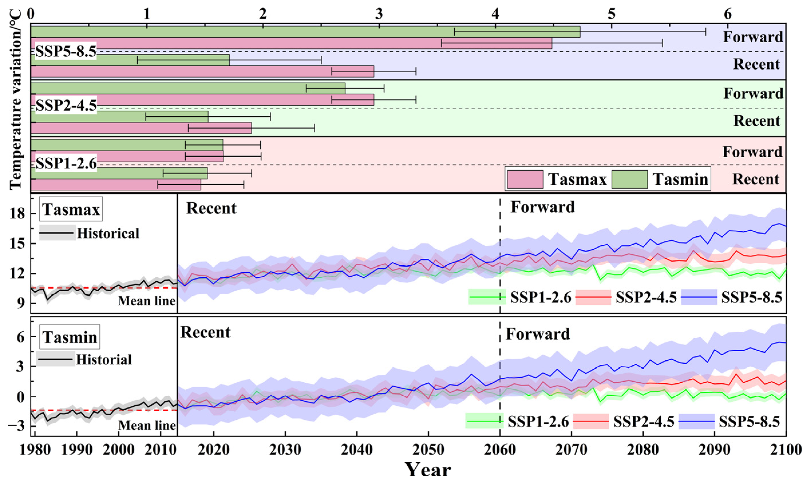
The annual temperature in the basin showed a fluctuating upward trend for the near (2015–2060) and the long future (2061–2100) (Figure 8), with the growth rate varying according to the forcing scenario and the occurrence period, and the upward trend gradually decreased in the order of high, medium, and low radiative forcing scenarios. The minimum temperature increase was greater than the maximum temperature increase, resulting in a gradual reduction in future temperature differences.

Figure 8.
The changes in future air temperature in the Manas River Basin compared with the historical period (1979–2014) and the time changes in annual average temperature during the period of 2015–2100 under different climate scenarios.
Under scenario SSP1-2.6, the temperature rise was relatively gentle, and the minimum temperature increased by 1.521 and 1.654 °C on average in the near and long term, respectively. The maximum temperature increased by 1.464 and 1.657 °C on average in the near and long term, respectively. Under this scenario, the long-term increase in maximum and minimum temperature was larger than the recent increase, and the maximum temperature increase was slightly larger than the minimum temperature increase.
Under scenario SSP2-4.5, temperature increased at a moderate rate, and the minimum temperature increased by 1.528 and 2.707 °C on average in the near and long term, respectively. The maximum temperature in the near and long term increased by 1.900 and 2.954 °C on average, respectively. For the near future, the maximum and minimum temperature rose at 0.04 and 0.037 °C/a, respectively, similar to the temperature rise in the observed historical period. The future and long-term rising speed decreased, and both were 0.015 °C/a. Under this scenario, the maximum temperature increase was greater than the minimum temperature increase, but the minimum temperature increases gradually rose from recent to long-term, basically the same as the maximum temperature increase.
Under scenario SSP5-8.5, both the temperature rise rate and the fluctuation range of future temperature reached maxima, and the minimum temperature increased by 1.710 and 4.729 °C on average in the near and long terms, respectively. The maximum temperature for the near and long term increased by 2.954 and 4.486 °C on average. The minimum temperature reached 0.272 °C in 2043, and the upper limit of the model exceeded 0 °C and reached 5.37 °C in 2100, indicating that the annual average minimum temperature of the basin will not be lower than 0 °C after 2043. At the same time, the maximum temperature growth rate gradually stabilized, and the near-term and long-term growth rates were 0.052 and 0.078 °C/a, respectively. The minimum temperature growth rate reached a peak value under the three scenarios, with near- and long-term growth rates of 0.061 and 0.096 °C/a, respectively. The long-term minimum temperature gradually exceeded the maximum temperature increase, which was 0.243 °C higher than the long-term maximum temperature increase, and the basin gradually developed into “warm and humid”.
3.2.2. Temperature Spatiotemporal Distribution Change
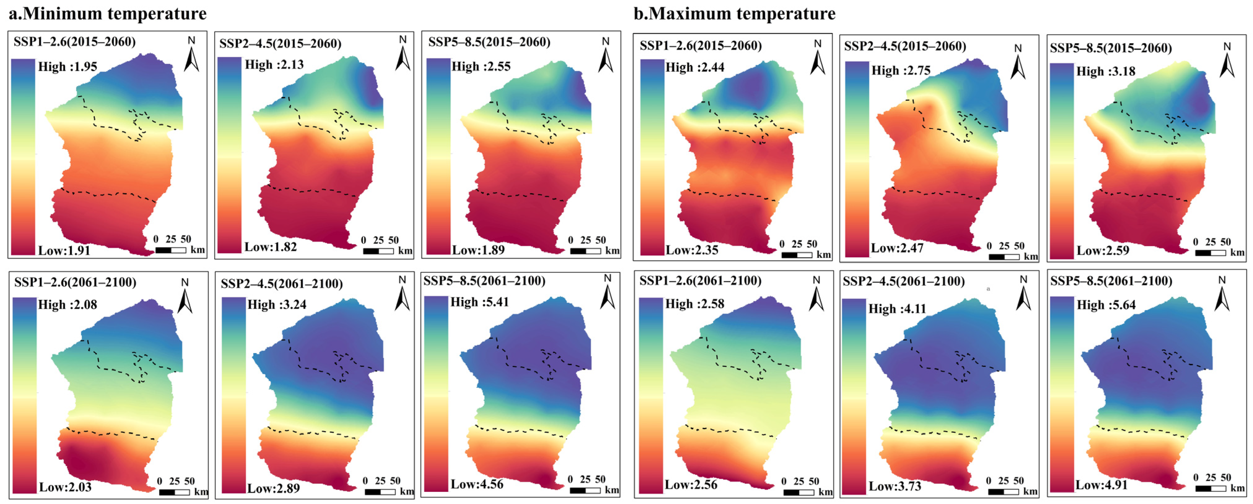
With 1979–2014 as the historical base period, the spatial distribution of temperature under the three different scenarios changed with time from north to south (Figure 9). Under scenarios SSP1-2.6, SSP2-4.5, and SSP5-8.5, the temperature increased continuously from south to north. The minimum temperature changes were 1.91–2.08, 1.82–3.24, and 1.89–5.41 °C, respectively, and the maximum temperature changes were 2.35–2.58, 2.47–4.11, and 2.59–5.64 °C. Combined with Figure 1, this trend shows that the distribution was mainly related to altitude and topography. The landform of the Manas River Basin from south to north proceeds in the order of mountain, plain, and desert, and the high-value centers are mainly deserts at low altitudes. This is because desert areas are not covered by vegetation and have strong evapotranspiration, which leads to a rapid warming speed. The low-value center is the mountain area with higher elevation, which is covered with a large amount of glaciers and snow, which is one reason for the small increase in temperature in this area.
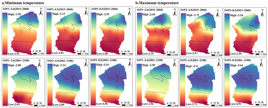
Figure 9.
Spatiotemporal distribution of future maximum/minimum temperature changes under different SSP-RCP scenarios.
Compared with the spatial changes in temperature under the three scenarios, the long-term temperature increased the most in scenario SSP5-8.5, with a maximum change of 5.64 °C. The minimum temperature increased more than the maximum temperature, consistent with the previous analysis results. A longitudinal comparative analysis of recent and long-term temperature extremes (maximum and minimum) revealed a spatial pattern of progressively higher warming rates from desert to oasis to mountainous zones. Concurrently, a gradual temperature elevation across the basin diminished the intra-basin temperature gradient while fostering an overall thermal intensification trend.
3.3. Temporal and Spatial Changes in Precipitation in Future Climate Scenarios
3.3.1. Precipitation Time Variation
Annual precipitation showed an increasing trend of fluctuation in the next two periods, and there was a clear increasing trend in precipitation in the near- and long-term future. The upward trend in the order of high, medium, and low radiative forcing scenarios gradually decreased, and the fluctuation range of precipitation also increased with the increase in time (Figure 10). The increasing trend in precipitation in the near future was small, with no significant difference in precipitation under the three forcing scenarios. Compared with the change in precipitation in the long-term future and the historical base period, there was little difference in the increase in the three forcing scenarios in the near future, unlike the temperature change in the near future.
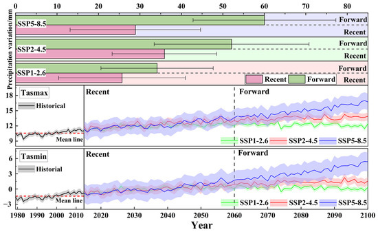
Figure 10.
The change in future precipitation in the Manas River Basin compared with the historical period (1979–2014) and the time change in annual precipitation for 1979–2100 under different climate scenarios.
Under scenario SSP1-2.6, the average precipitation in the near- and long-term future reached 288.80 and 298.07 mm, respectively, with increases of 8.88% and 11.01% compared with the historical average, and the precipitation increments were 25.69 and 34.14 mm, respectively. Under scenario SSP2-4.5, the average precipitation for the near- and long-term future was 297.68 and 316.04 mm, respectively, with increases of 10.06% and 16.85% compared with the historical average. The precipitation increments were 35.91 and 52.11 mm, respectively. Under scenario SSP5-8.5, the change trend in precipitation in the near future slightly differed from that under scenarios SSP2-4.5 and SSP1-2.6. Precipitation in the long term began to increase at a rate of 1.42 mm/a, and the increment was 60.03 mm, more than twice the recent increment. In 2095, the maximum precipitation was 355.75 mm. Unlike temperature, the variation range of precipitation was negative, and the fluctuation range was −42.66 to 51.72 mm, indicating a decrease in precipitation.
3.3.2. Precipitation Spatiotemporal Distribution Change
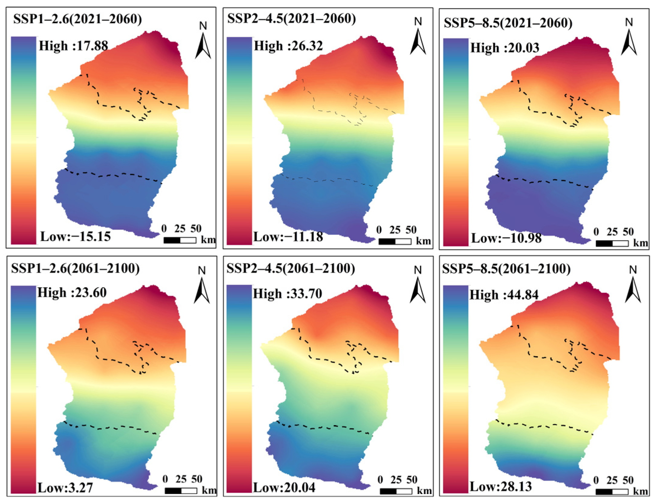
The distribution of precipitation increase is greatly affected by altitude and terrain, and the desert area was the low-value center of precipitation increase. But, with an increase in altitude, the precipitation increase gradually rose, and the high-value center of precipitation increase formed in the mountain area (Figure 11). The precipitation increase in the mountain area underwent a large change, while that in the desert and plain areas underwent a small change. This contrasts with the spatial distribution of the future temperature increase.
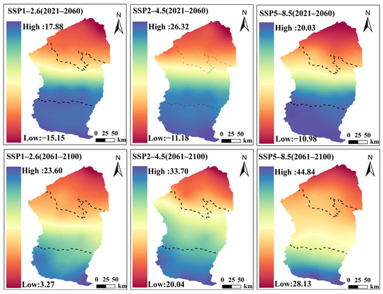
Figure 11.
Spatiotemporal distribution of future precipitation changes under different SSP-RCP scenarios.
Under scenarios SSP1-2.6, SSP2-4.5, and SSP5-8.5, the precipitation variations were −15.15 to 23.60, −11.18 to 33.70, and −10.98 to 44.84 mm, respectively. In the near future, the precipitation in the basin was all negative. In the desert area of the basin, precipitation decreased from 2015 to 2060, and the maximum precipitation variation under scenario SSP2-4.5 was 37.5 mm, while the precipitation variation in scenario SSP5-8.5 declined to 31.01 mm. In the long term, the spatial change in the precipitation increase was not as drastic as for the recent period, and precipitation gradually increased, but the precipitation difference gradually tended to be stable. The decrease in the water increment difference under scenario SSP1-2.6 was 20.33 mm, while that in scenario SSP5-8.5 was 16.71 mm.
The spatial distribution of the precipitation increase for the future was consistent with the spatial distribution of the precipitation in the historical period. The precipitation and precipitation increase values for the low-altitude area were small, and the precipitation and precipitation increase values for the high-altitude area were large. This distribution feature is consistent with the physical mechanism of the topographic uplift effect and has been independently verified by the HRLT high-resolution dataset [25]. Moreover, it is in line with the research conclusions of adjacent arid inland river basins (such as the Hetian River and the Shiyang River) [52,53], further supporting the long-term dominant impact of topography on the spatial pattern of precipitation.
3.4. Comparison with Other Inland River Basins in Northwest China
The GCM is a complex mathematical and physical model that simulates these three multi-dimensional dynamics of the Earth’s atmosphere, oceans, and land surface [10]. The results of this study show that the model data, after bias correction, have greatly improved the accuracy of the model, and RF has the best performance, but there are still some models with poor fitting to the observed data. After removing the models with poor performance, WSM is used to forecast the three scenarios in the future. The overall performance changes with time, and the future precipitation increases gradually from south to north. The temperature increases gradually from north to south. In the SSP5.8-5 scenario, the long-term minimum temperature increase is gradually greater than the maximum temperature increase, and the annual average minimum temperature will not be lower than 0 °C after 2043, and the basin will gradually develop into “warm and humid”.
Although the climate model has a certain simulation ability in the Manas River Basin, there are great differences among the models, and the simulation effect of the climate model on different time scales is better than that of the precipitation simulation, which is consistent with the results of many studies [54,55]. The Manas River Basin, as a typical arid inland river basin, has obvious regional characteristics. Glacier snowmelt in the alpine mountains is used in the oasis area and dissipated in the desert area. The changes in temperature and precipitation are consistent with the regional characteristics of the river basin [56]. At the same time, some studies show that the increase in the minimum temperature is more gradual than that in the maximum temperature trend. This indicates that, under the influence of the global greenhouse effect, the phenomenon of increasing temperature and decreasing temperature difference year by year is more and more significant [57,58].
Compared with previous research achievements in arid inland river basins in China, Chaofei He [52] found that the temperature of the Hetian River Basin is higher than that reported in this study. This is because the area in the Hetian River Basin has a lower altitude, drier climate, lower vegetation coverage rate, less cloud cover, and higher surface albedo due to the influence of surrounding deserts and other natural environments. This leads to direct sunlight on the ground; faster warming is consistent with the actual situation. The precipitation in the Shiyang River Basin [53] is lower than the precipitation reported in this study. The large amount of glaciers and snow cover in the Manas River Basin is due to the high altitude of the mountain area of the basin as well as the special geographical location. As the altitude increases, the precipitation increases gradually, and a high-value center of increase is formed in the high mountain area covered by glaciers and snow. This makes the alpine mountains more sensitive to climate. The increasing trend in regional temperature leads to the melting of glaciers and snow in the basin, which makes the local climate warm and humid and increases precipitation, thus further affecting the amount of water resources in glacier-fed rivers [59].
4. Conclusions
This study provides a comprehensive assessment of future climate change impacts on the Manas River Basin, an arid inland region in northwestern China, by integrating nine CMIP6 models with advanced MME techniques. WSM effectively reduces uncertainties. Our key findings reveal distinct climate trajectories under different SSPs. Under the low-forcing SSP1-2.6 scenario, the basin is projected to experience moderate warming, with long-term increases of 1.654 °C in maximum temperature, 1.657 °C in minimum temperature, and 34.137 mm in precipitation, accompanied by minimal climate variability. In contrast, the high-forcing SSP5-8.5 scenario exhibits the most pronounced changes, with maximum and minimum temperatures rising by 4.485 °C and 4.728 °C, respectively, and precipitation increasing by 60.035 mm by 2100.
High-altitude precipitation increases stem from orographic uplift-driven adiabatic cooling, while low deserts lack such dynamics. Rising greenhouse gases reduce nocturnal radiative cooling, causing greater minimum than maximum temperature increases. Notably, the minimum temperature increment surpasses the maximum temperature after 2043, signaling a transition toward a warmer and more humid climate regime. Spatially, warming hotspots are concentrated in low-altitude desert areas due to reduced vegetation cover and intensified evapotranspiration, while precipitation increases correlate strongly with elevation, peaking in mountainous regions. This spatial heterogeneity underscores the critical role of topography in modulating regional climate responses. Such shifts pose dual challenges and opportunities for sustainable water resource management, agricultural productivity, and ecosystem resilience. Adaptive strategies, including optimized irrigation systems, alpine water source conservation, and drought-resistant crop cultivation, are imperative to mitigate risks from extreme climate events and shifting hydrological patterns. These advancements will be critical for informing climate-resilient policies and fostering sustainable development in arid inland river basins under escalating global warming.
While this study highlights the efficacy of WSM and machine learning in reducing climate projection uncertainties, limitations persist. The selected SSP scenarios, while covering a broad range of radiative forcing levels, exclude intermediate or regionally tailored pathways, potentially overlooking socioeconomic or policy-driven climate trajectories specific to arid inland basins. Structural uncertainties persist due to shared parameterizations among the CMIP6 models, despite prioritizing independent models, which may amplify biases in extreme precipitation projections. Additionally, the reliance on 0.5° × 0.5° gridded data limits the resolution of localized microclimates, particularly at mountain–desert interfaces, while the focus on mean climate trends omits compound extremes critical for agricultural risk assessment. Future efforts should integrate higher-resolution regional climate models, hybrid dynamical–statistical downscaling, and extreme event indices (e.g., CDD, R×5day) to enhance spatial fidelity and risk quantification. Coupling these advancements with hydrological models could further bridge the gap between climate projections and adaptive water management strategies, ensuring robust policymaking in the face of escalating aridification.
Supplementary Materials
The following supporting information can be downloaded at: https://www.mdpi.com/article/10.3390/su17083658/s1, Text S1 Description of Data Sources; Text S2 Description of Random forest(RF) practices; Text S3 Description of Artificial neural network(ANN) practices; Text S4 Description of Support Vector Machine(SVM) practices; Text S5 Data comparison before and after quantile mapping processing; Table S1 Details of observed data; Table S2 Climate model information; Table S3 Random Forest model parameter setting table; Table S4 Artificial Neural Network model parameter setting table; Table S5 Support Vector Machine model parameter setting table;Table S6 The correlation coefficient (r), mean absolute error (MAE) and root mean square error (RMSD) of maximum and minimum temperature and precipitation on monthly scale were compared before and after correction; Table S7 Data needed to draw Taylor diagrams; Figure S1. Interannual variation curves of the models and observed values before and after correction for minimum and maximum temperature and precipitation.
Author Contributions
F.Z. conceived the experiments, analyzed the results, and wrote the manuscript. X.H. conceived the experiments, analyzed the results, and wrote and revised the manuscript. G.Y. provided important feedback, making the article more complete. X.H. reviewed the article and provided suggestions. X.L. edited and reviewed the manuscript. All authors have read and agreed to the published version of the manuscript.
Funding
This research was funded by The Key Field Science and Technology Research Project of Xinjiang Uygur Autonomous Region Corps (Project No. 2023AB059).
Institutional Review Board Statement
Not applicable.
Informed Consent Statement
Not applicable.
Data Availability Statement
The data used in this study are sourced from the World Climate Research Programme’s Working Group on Coupled Modelling and are freely available through the Earth System Grid Federation (ESGF) at https://esgf-index1.ceda.ac.uk/search/cmip6-ceda/, accessed on 10 October 2024. HRLT data from Earth & Environmental Science, Accessible at https://doi.pangaea.de/10.1594/PANGAEA.941329?format=html#download, accessed on 10 October 2024.
Acknowledgments
We acknowledge the data support from Qin and Zhang [28] (https://doi.pangaea.de/10.1594/PANGAEA.941329?format=html#download (Accessed on 10 October 2024.)) and Lawrence Livermore National Laboratory, LLNL (https://esgf-index1.ceda.ac.uk/projects/cmip6-ceda/ (Accessed on 10 October 2024.)).
Conflicts of Interest
The authors declare no conflict of interest.
References
- Wang, Y.; Wang, J.; Zhang, Q. Analysis of ecological drought risk characteristics and leading factors in the Yellow River Basin. Theor. Appl. Climatol. 2023, 155, 1739–1757. [Google Scholar] [CrossRef]
- Sun, F. Analysis of Short-Term Heavy Rainfall-Based Urban Flood Disaster Risk Assessment Using Integrated Learning Approach. Sustainability 2024, 16, 8249. [Google Scholar] [CrossRef]
- Singh, H.V.; Joshi, N.; Suryavanshi, S. Projected climate extremes over agro-climatic zones of Ganga River Basin under 1.5, 2, and 3° global warming levels. Environ. Monit. Assess. 2023, 195, 1062. [Google Scholar] [CrossRef] [PubMed]
- Potopová, V.; Trifan, T.; Trnka, M.; De Michele, C.; Semerádová, D.; Fischer, M.; Meitner, J.; Musiolková, M.; Muntean, N.; Clothier, B. Copulas modelling of maize yield losses—Drought compound events using the multiple remote sensing indices over the Danube River Basin. Agric. Water Manag. 2023, 280, 108217. [Google Scholar] [CrossRef]
- Pawankar, R.; Akdis, C.A. Climate change and the epithelial barrier theory in allergic diseases: A One Health approach to a green environment. Allergy 2023, 78, 2829–2834. [Google Scholar] [CrossRef]
- Wang, J.; Chen, G.; Yuan, Y.; Fei, Y.; Xiong, J.; Yang, J.; Yang, Y.; Li, H. Spatiotemporal changes of ecological environment quality and climate drivers in Zoige Plateau. Environ. Monit. Assess. 2023, 195, 912. [Google Scholar] [CrossRef]
- Zhou, T.; Zou, L.; Chen, X. Commentary on the Coupled Model Intercomparison Project Phase 6 (CMIP6). Clim. Chang. Res. 2019, 15, 445–456. [Google Scholar]
- Salehie, O.; Hamed, M.M.; Ismail, T.b.; Tam, T.H.; Shahid, S. Selection of CMIP6 GCM with projection of climate over the Amu Darya River Basin. Theor. Appl. Climatol. 2022, 151, 1185–1203. [Google Scholar] [CrossRef]
- Crévolin, V.; Hassanzadeh, E.; Bourdeau-Goulet, S.-C. Updating the intensity-duration-frequency curves in major Canadian cities under changing climate using CMIP5 and CMIP6 model projections. Sustain. Cities Soc. 2023, 92, 104473–104489. [Google Scholar] [CrossRef]
- Song, Y.H.; Chung, E.-S.; Shahid, S. Spatiotemporal differences and uncertainties in projections of precipitation and temperature in South Korea from CMIP6 and CMIP5 general circulation models. Int. J. Climatol. 2021, 15, 215–229. [Google Scholar] [CrossRef]
- Jiang, Z.; Li, W.; Xu, J.; Li, L. Extreme Precipitation Indices over China in CMIP5 Models. Part I: Model Evaluation. Am. Meteorol. Soc. 2015, 10, 1–44. [Google Scholar] [CrossRef]
- Ghaemi, A.; Monfared, S.A.H.; Bahrpeyma, A.; Mahmoudi, P.; Zounemat-Kermani, M. Exploitation of the ensemble-based machine learning strategies to elevate the precision of CORDEX regional simulations in precipitation projection. Earth Sci. Inform. 2024, 17, 1373–1392. [Google Scholar] [CrossRef]
- Dawkins, L.C.; Bernie, D.J.; Lowe, J.A.; Economou, T. Assessing climate risk using ensembles: A novel framework for applying and extending open-source climate risk assessment platforms. Clim. Risk Manag. 2023, 40, 100510. [Google Scholar] [CrossRef]
- Shiva, J.S.; Chandler, D.G. Projection of Future Heat Waves in the United States. Part I: Selecting a Climate Model Subset. Atmosphere 2020, 11, 587. [Google Scholar] [CrossRef]
- Sanderson, B.M.; Knutti, R.; Caldwell, P. Addressing interdependency in a multimodel ensemble by interpolation of model properties. Am. Meteorol. Soc. 2015, 28, 5150–5170. [Google Scholar] [CrossRef]
- Salcedo-Sanz, S.; Pérez-Aracil, J.; Ascenso, G.; Ser, J.D.; Casillas-Pérez, D.; Kadow, C.; Fister, D.; Barriopedro, D.; García-Herrera, R.; Giuliani, M.; et al. Analysis, characterization, prediction, and attribution of extreme atmospheric events with machine learning and deep learning techniques: A review. Theor. Appl. Climatol. 2024, 155, 1–44. [Google Scholar] [CrossRef]
- Chen, Y.; Wang, N.; Jiao, J.; Li, J.; Bai, L.; Liang, Y.; Wei, Y.; Zhang, Z.; Xu, Q.; Zhang, Z.; et al. Predicting soil loss in small watersheds under different emission scenarios from CMIP6 using random forests. Earth Surf. Process. Landf. 2024, 49, 4469–4484. [Google Scholar] [CrossRef]
- Dey, A.; Sahoo, D.P.; Kumar, R.; Remesan, R. A multimodel ensemble machine learning approach for CMIP6 climate model projections in an Indian River basin. Int. J. Climatol. 2022, 42, 9215–9236. [Google Scholar] [CrossRef]
- Karimizadeh, K.; Yi, J. Modeling Hydrological Responses of Watershed Under Climate Change Scenarios Using Machine Learning Techniques. Water Resour. Manag. 2023, 37, 5235–5254. [Google Scholar] [CrossRef]
- O’Gorman, P.A.; Dwyer, J.G. Using Machine Learning to Parameterize Moist Convection: Potential for Modeling of Climate, Climate Change, and Extreme Events. J. Adv. Model. Earth Syst. 2018, 10, 2548–2563. [Google Scholar] [CrossRef]
- Sachindra, D.A.; Ahmed, K.; Rashid, M.M.; Shahid, S.; Perera, B.J.C. Statistical downscaling of precipitation using machine learning techniques downscaling with machine learning techniques. Atmos. Res. 2018, 212, 240–258. [Google Scholar] [CrossRef]
- Gumus, V.; El Moçayd, N.; Seker, M.; Seaid, M. Evaluation of future temperature and precipitation projections in Morocco using the ANN-based multi-model ensemble from CMIP6. Atmos. Res. 2023, 292, 106880. [Google Scholar] [CrossRef]
- Yu, P.; Xu, H.; Liu, S.; Qiao, M.; Zhang, Q.; An, H.; Fu, J. Spatial distribution pattern changes of oasis soil types in Manasi River Basin, arid northwestern China. Catena 2011, 87, 253–259. [Google Scholar] [CrossRef]
- Shang, H.; Wang, W.; Dai, Z.; Duan, L.; Zhao, Y.; Zhang, J. An ecology-oriented exploitation mode of groundwater resources in the northern Tianshan Mountains, China. J. Hydrol. 2016, 54, 386–394. [Google Scholar] [CrossRef]
- Qin, R.; Zhang, F. HRLT: A high-resolution (1 day, 1 km) and long-term (1961–2019) gridded dataset for temperature and precipitation across China. Earth Syst. Sci. Data 2022, 14, 4793–4810. [Google Scholar] [CrossRef]
- Feng, M.; Sexton, J.O.; Channan, S.; Townshend, J.R. A global, high-resolution (30-m) inland water body dataset for 2000: First results of a topographic–spectral classification algorithm. Int. J. Digit. Earth 2015, 9, 113–133. [Google Scholar] [CrossRef]
- He, J.; Yang, K.; Tang, W.; Lu, H.; Qin, J.; Chen, Y.; Li, X. The first high-resolution meteorological forcing dataset for land process studies over China. Sci. Data 2020, 7, 25. [Google Scholar] [CrossRef]
- Qian, Y.; Zou, H.; Hong, M. Evaluating the evolution of wind energy resource in the Northwest Passage under climate change based on CMIP5 models. Mar. Forecast. 2021, 38, 76–86. [Google Scholar]
- Li, X.; Li, Z. Evaluation of bias correction techniques for generating high-resolution daily temperature projections from CMIP6 models. Clim. Dyn. 2023, 61, 3893–3910. [Google Scholar] [CrossRef]
- Xue, P.; Zhang, C.; Wen, Z.; Park, E.; Jakada, H. Climate variability impacts on runoff projection under quantile mapping bias correction in the support CMIP6: An investigation in Lushi basin of China. J. Hydrol. 2022, 614, 128550. [Google Scholar] [CrossRef]
- Tadase, A.T. Climate trend analysis in the ramis catchment, upper wabi shebelle basin, Ethiopia, using the CMIP6 dataset. J. Afr. Earth Sci. 2024, 217, 105347. [Google Scholar] [CrossRef]
- Niranjan Kumar, K.; Thota, M.S.; Ashrit, R.; Mitra, A.K.; Rajeevan, M.N. Quantile mapping bias correction methods to IMDAA reanalysis for calibrating NCMRWF unified model operational forecasts. Hydrol. Sci. J. 2022, 67, 870–885. [Google Scholar] [CrossRef]
- Zhang, Q.; Gan, Y.; Zhang, L.; She, D.; Wang, G.; Wang, S. Piecewise-quantile mapping improves bias correction of global climate model daily precipitation towards preserving quantiles and extremes. Int. J. Climatol. 2022, 42, 7968–7986. [Google Scholar] [CrossRef]
- Wang, Z.; Gong, H.; Huang, M.; Gu, F.; Wei, J.; Guo, Q.; Song, W. A multimodel random forest ensemble method for an improved assessment of Chinese terrestrial vegetation carbon density. Methods Ecol. Evol. 2021, 14, 117–132. [Google Scholar] [CrossRef]
- Costache, R.; Arabameri, A.; Elkhrachy, I.; Ghorbanzadeh, O.; Pham, Q.B. Detection of areas prone to flood risk using state-of-the-art machine learning models. Geomat. Nat. Hazards Risk 2021, 12, 1488–1507. [Google Scholar] [CrossRef]
- Than, N.H.; Ly, C.D.; Tat, P.V. The performance of classification and forecasting Dong Nai River water quality for sustainable water resources management using neural network techniques. J. Hydrol. 2021, 596, 126099. [Google Scholar] [CrossRef]
- Jalili, A.A.; Najarchi, M.; Shabanlou, S.; Jafarinia, R. Multi-objective Optimization of water resources in real time based on integration of NSGA-II and support vector machines. Environ. Sci. Pollut. Res. 2023, 30, 16464–16475. [Google Scholar] [CrossRef]
- Li, T.; Jiang, Z.; Treut, H.L.; Li, L.; Zhao, L.; Ge, L. Machine learning to optimize climate projection over China with multi-model ensemble simulations. Environ. Res. Lett. 2021, 16, 28–44. [Google Scholar] [CrossRef]
- Fan, X.; Miao, C.; Duan, Q.; Shen, C.; Wu, Y. The Performance of CMIP6 Versus CMIP5 in Simulating Temperature Extremes Over the Global Land Surface. J. Geophys. Res. Atmos. 2020, 125, 1–16. [Google Scholar] [CrossRef]
- Yang, X.; Zhou, B.; Xu, Y.; Han, Z. CMIP6 Evaluation and Projection of Temperature and Precipitation over China. Adv. Atmos. Sci. 2021, 38, 817–830. [Google Scholar] [CrossRef]
- Hamed, M.M.; Nashwan, M.S.; Shahid, S.; Ismail, T.b.; Wang, X.; Dewan, A.; Asaduzzaman, M. Inconsistency in historical simulations and future projections of temperature and rainfall: A comparison of CMIP5 and CMIP6 models over Southeast Asia. Atmos. Res. 2022, 265, 105927–105940. [Google Scholar] [CrossRef]
- Zhang, Y.; You, Q.; Chen, C.; Ge, J.; Adnan, M. Evaluation of Downscaled CMIP5 Coupled with VIC Model for Flash Drought Simulation in a Humid Subtropical Basin, China. J. Clim. 2018, 31, 31. [Google Scholar] [CrossRef]
- Taylor, K.E. Summarizing multiple aspects of model perform-ance in a single diagram. J. Geophys. Res. Atmos. 2001, 106, 7183–7192. [Google Scholar] [CrossRef]
- de Souza, L.S.; da Silva, M.S.; de Almeida, V.A.; Moraes, N.O.; de Souza, E.P.; Senna, M.C.; França, G.B.; Frota, M.N.; de Almeida, M.V.; Viana, L.Q. Evaluation of Cumulus and Microphysical Parameterization Schemes of the WRF Model for Precipitation Prediction in the Paraíba do Sul River Basin, Southeastern Brazil. Pure Appl. Geophys. 2024, 181, 679–700. [Google Scholar] [CrossRef]
- Luo, N.; Guo, Y.; Chou, J.; Gao, Z. Added value of CMIP6 models over CMIP5 models in simulating the climatological precipitation extremes in China. Int. J. Climatol. 2021, 42, 1148–1164. [Google Scholar] [CrossRef]
- Sun, L.; Lan, Y.; Jiang, R. Using CNN framework to improve multi-GCM ensemble predictions of monthly precipitation at local areas: An application over China and comparison with other methods. J. Hydrol. 2023, 623, 129866. [Google Scholar] [CrossRef]
- Ma, S.; Chen, C.; Zhi, X.; He, H.; Wu, D. The assessment and verification of convection-allowing ensemble forecast based on spatial-temporal uncertainties. Acta Meteorol. Sin. 2018, 76, 578–589. [Google Scholar]
- Maghrebi, M.F.; Vatanchi, S.M.; Kawanisi, K. Investigation of stage-discharge model performance for streamflow estimating: A case study of the Gono River, Japan. River Res. Appl. 2023, 39, 805–818. [Google Scholar] [CrossRef]
- Mo, C.; Liu, G.; Lei, X.; Zhang, M.; Ruan, Y.; Lai, S.; Xing, Z. Study on the Optimization and Stability of Machine Learning Runoff Prediction Models in the Karst Area. Appl. Sci. 2022, 12, 4979. [Google Scholar] [CrossRef]
- Jiang, F.; Hu, R.; Yang, Y. Abrupt Change in the Time Sequences of Flood Disastersin Xinjiang and Its Possible Climatic Reasons. J. Glaciol. Geocryol. 2004, 26, 674–681. [Google Scholar]
- Zou, Q.; Wang, G.; He, B.; Shen, Y. Responding of Summer Runoff and Flood Processes to Extreme Climate Events in Manas River Basin, Tianshan Mountains during 1957–2010. J. Glaciol. Geocryol. 2013, 35, 733–740. [Google Scholar]
- He, C.; Luo, C.; Chen, F.; Long, A.; Tang, H. Prediction of future climate change in Hetian River Basin based on CMIP6 multi-model. Earth Sci. Front. 2023, 30, 515–528. [Google Scholar]
- Jun, D.A.; Haizhu, H.U.; Xiaomin, M.A.; Ji, Z.H. Future climate change trends in the Shiyang River Basin based on the CMIP6 multi-model estimation data. Arid Zone Res. 2023, 40, 1547–1562. [Google Scholar]
- Ma, F.; Yuan, X.; Liu, X. Intensification of drought propagation over the Yangtze River basin under climate warming. Int. J. Climatol. 2023, 43, 5640–5661. [Google Scholar] [CrossRef]
- Reder, A.; Raffa, M.; Montesarchio, M.; Mercogliano, P. Performance evaluation of regional climate model simulations at different spatial and temporal scales over the complex orography area of the Alpine region. Nat. Hazards 2020, 102, 151–177. [Google Scholar] [CrossRef]
- Gu, X. Response of Runoff to Climate Change in Runoff Producing area of Manasi River Basin. Master Thesis, Shihezi University, Shihezi, China, 2021. [Google Scholar]
- Donk, P.; Van Uytven, E.; Willems, P.; Taylor, M.A. Assessment of the potential implications of a 1.5 °C versus higher global temperature rise for the Afobaka hydropower scheme in Suriname. Reg. Environ. Chang. 2018, 18, 2283–2295. [Google Scholar] [CrossRef]
- Niroumand Fard, F.; Khashei Siuki, A.; Hashemi, S.R.; Ghorbani, K. Evaluation of the effect of scenarios in the 6th report of IPCC on the prediction groundwater level using the non-linear model of the input-output time series. Environ. Monit. Assess. 2023, 195, 1359. [Google Scholar] [CrossRef]
- Li, C.; Hao, J.; Zhang, G.; Fang, H.; Wang, Y.; Lu, H. Runoff variations affected by climate change and human activities in Yarlung Zangbo River, southeastern Tibetan Plateau. Catena 2023, 230, 107184. [Google Scholar] [CrossRef]


Disclaimer/Publisher’s Note: The statements, opinions and data contained in all publications are solely those of the individual author(s) and contributor(s) and not of MDPI and/or the editor(s). MDPI and/or the editor(s) disclaim responsibility for any injury to people or property resulting from any ideas, methods, instructions or products referred to in the content. |
© 2025 by the authors. Licensee MDPI, Basel, Switzerland. This article is an open access article distributed under the terms and conditions of the Creative Commons Attribution (CC BY) license (https://creativecommons.org/licenses/by/4.0/).