Abstract
The article discusses the application of advanced data mining methods applicable to electricity consumption within a local power system in Poland. This analysis involves power demand. It is aimed at predicting daily demand variations. In such a case, system demand is characterized by high variability over a short period of time, e.g., 24 h. This constitutes a significant issue within a small power grid. It entails effective load programming on a given day and time. Therefore, the authors of the paper suggested employing artificial intelligence to forecast industrial power grid load for successive time intervals of the operation process. Such a solution applied within a power system enables appropriate start-up/shut-down planning, as well as generator operation at a specific capacity in power plants. It thus allows continuous power system (on-line) load demand balancing. Predicting power system load also involves determining moments, e.g., of power plant start-up, transition times to maximum or minimum output, or also the shut-down of such a process. This means ongoing and continuous (automatic) impact on electricity distribution. It significantly reduces carbon dioxide atmospheric emissions and allows zero-emission, e.g., wind, hydro, geothermal, or solar plants to meet current power needs. The issue associated with operating small ‘island’ power systems is a dynamic and rapid change in power demand. This is related to the area-based—‘island’—use’ of available power sources that can only be operated within a specific area. A very important problem occurring within these structurally small grids is the continuous forecasting of load changes and real-time response to power demand (i.e., balancing power demand through in-house or available power sources).
1. Introduction
The power grid of a specific country is a combination of conduits, overhead or underground electric tractions, or other functionally related equipment that converts electricity, e.g., transformers and switching stations, etc. [1,2,3]. All these components or devices are electrically coupled, which means they form an always-oriented connection network with specific, assigned relations, e.g., power plant—high-voltage line—transformer station—power consumer [4,5,6,7]. National power systems are intended to transmit (power lines, PL), convert (transformer stations, TS), and distribute (switching stations, SS) electricity generated in emission-generating and zero-emission power plants (Figure 1) over a specific area. Electricity is sent to all users, i.e., consumers, e.g., residents, industrial plants, buildings, and state critical infrastructure facilities (SCIF), etc. [8,9,10,11,12]. Electricity generated in power plants is used to power all electrical and electronic consumers. It is essential for their operation and implementation of all programmed functionalities. The above components and devices comprise a specific power system employed within a given country and classified as SCIF [13,14,15,16,17,18,19]. A power system includes specific elements (such as PL, TS, or DS) that function as a whole. Those are interrelated elements. In other words, specific functional relations, e.g., TS—SS, PL—TS, etc., and feedback can be allotted within a power system. A power system (PS) is always internally and externally coordinated when interconnecting with a different national transmission system. A PS always forms a specific technical structure of connections, as well as reliability. It is a set of components and devices used online to transmit and distribute electricity. To improve electricity transmission reliability, a PS always includes an additional set of elements ensuring the so-called redundancy. Redundancy can be hot (operating at a given moment) or cold (planned for start-up due to a failure) [4,20,21,22,23,24,25,26].
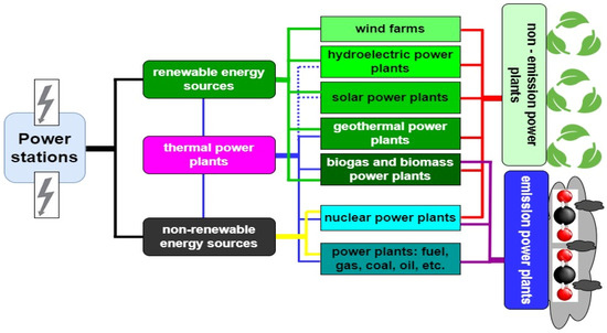
Figure 1.
Division of power plants operating within a given national PS, taking into account no emissions and active emissions of pollutants to the atmosphere (original study).
The following power plant types can be distinguished within a national power system—renewable and non-renewable; employing conversion to thermal energy within their process; as shown in Figure 1. Climate-related threats that are a current global challenge (ozone hole, climate change, etc.) drive the development of power plants classified as zero-emission, e.g., on- and off-shore wind farms, hydro, geothermal, and solar power plants—Figure 1. Power plants fired by non-renewable sources include two types of power facilities that utilize different materials to generate required heat and energy, namely, most usually coal and fissile fuel—Figure 1. A noteworthy parameter that characterizes all of the aforementioned power plants operating within a PS is the so-called inertia time (defined in electronic engineering as a time constant τ) of the response to power demand at a given moment [19,27,28,29,30,31,32,33,34]. It is a particularly important technical parameter that is employed to balance the power demand for a given PS, and at a specific moment in time, e.g., start-up, synchronization, connecting a different generator to the grid, and also reaching specific available capacity within the system required to meet the entire demand, etc.
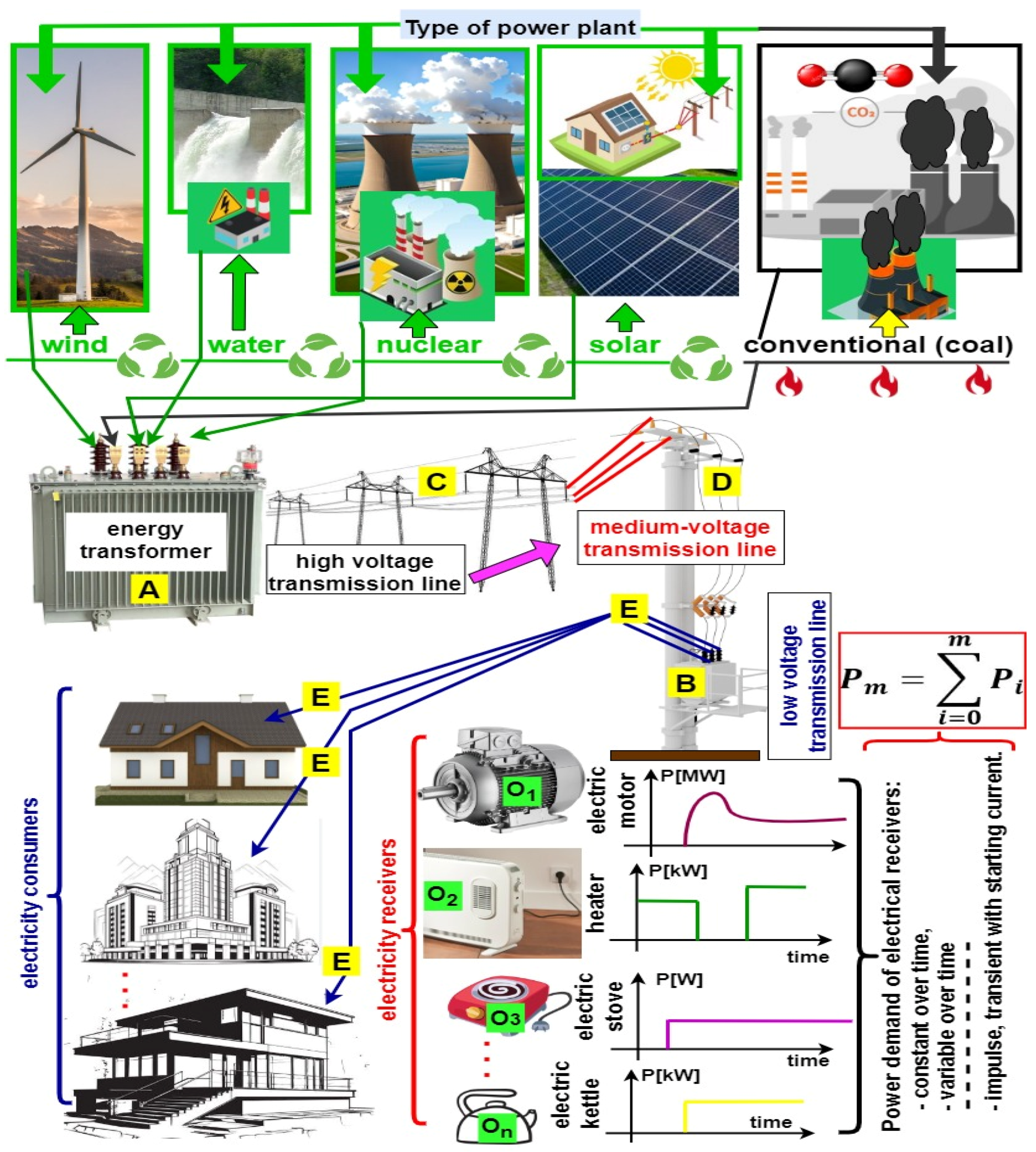
Figure 2 is a general illustration of a PS, including interlinks and relations between ST, SR, and LE. Due to the fact that they are being used to convert electricity, the O1, O2, O3, …, On consumers are characterized by different load parameters, including current consumption at time t. O consumers are located at geographically different sites within a given PS—Figure 2. There are also usually time-varying and variable (pulsed or constant) power demands of such equipment.
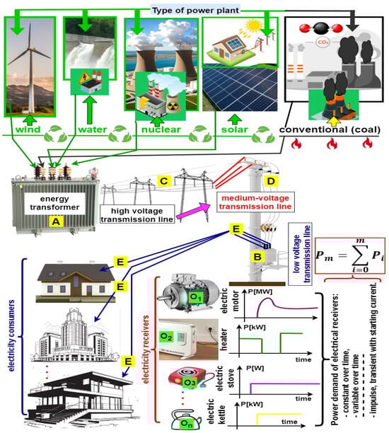
Figure 2.
Functional links within a real power system, where power lines are marked as follows: (C)—high voltage; (D)—medium voltage; (E)—low voltage; (A,B)—transformer stations O1, O2, O3, …, On—electricity consumers; Pm—system power demand; Pi—demand for power specifically determined by a given consumer in the system; m—number of consumers operating within a given power system (original study).
Electricity generated in a power plant by a high-voltage TS (A) is supplied to an overhead power grid. Via high- (C), medium- (D), or low-voltage (D) PL, it is then fed via a TS (B) to electricity consumers that usually exhibit a varying rated capacity: very high MW (106 W), medium kW (103 W), as well as low (W). Start-up (incorporation) characteristics, including specific consumers’ power demand, differ, as shown in Figure 2 [24,27,35,36]. They vary from pulsed current waveforms at an initial start-up time O1 to steady. Most often, other consumers have set power demand waveforms. Only pulsed changes, variable over demand time, most often appear at consumer start-up time O2, O3, …, On [11,26,37,38].
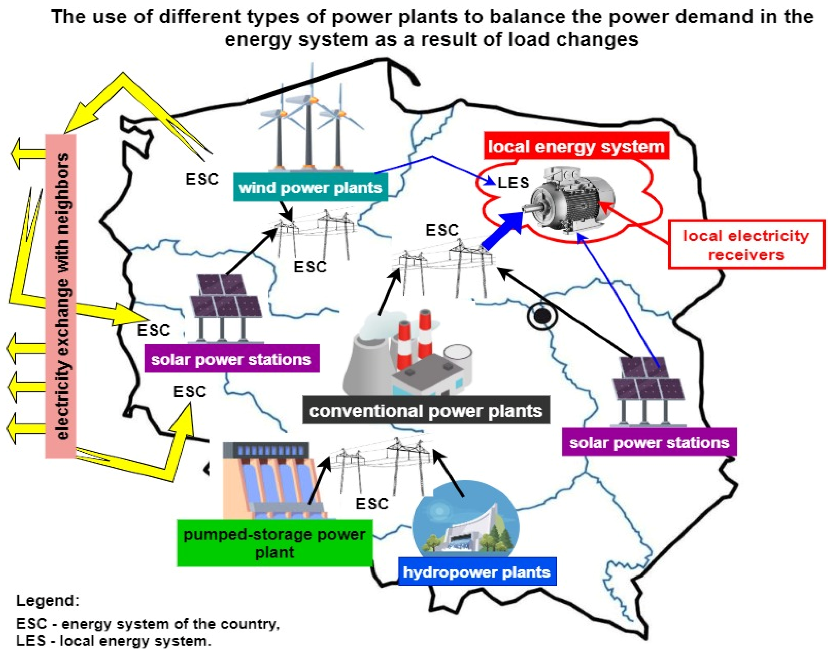
Therefore, predicting power demand employing different technical solutions, including the so-called artificial intelligence, is a burning issue related to operating power grids. It provides a real opportunity to impact electricity distribution throughout the system, limiting unnecessary consumption [8,39,40,41]. It is an actually applied way of limiting carbon dioxide emissions by power plants in the so-called small power grids—Figure 3. Another method to balance power demand is purchasing electricity from other systems—Figure 3. Small power systems (Figure 3) always include a finite, local number of electricity consumers. As shown in Figure 2, the power demand is the total power for individual consumers O1, O2, O3, …, On is also always characterized by a well-defined (usually known) variability over a given PS operation time. Demand variations and different electric consumer start-up times are reasons for PS load changes at a given moment and, thus, power demand at a given time t [21,28,42,43].
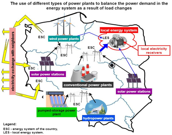
Figure 3.
Position of a local power system (LPS) within the NPS structure in Poland (original study).
The inclusion and possibility of determining and employing load predictions throughout the entire NPS, let alone an LPS, is always a function of response to instantaneous power demand for the power plant itself—Figure 4. This function also depends on the power plant technical parameters applied within a given PS, Figure 4. One of the key aspects in determining electricity demand in NPS and LPS is also the determined possible gradient of power demand changes over time, or the power change rate for a given time interval (response time to a change in input conditions—power demand). It is the magnitude of these changes, W, kW, or MW, at a given moment in time, as well as the determination of the minimum and maximum power within a given SE (cable cross-section, permissible voltage dips in a PS, etc.). Figure 4 illustrates the rate of power plant load (response) change depending on the electricity generation technology employed [12,20,44,45,46]. The power plant that is characterized by the highest rate of such changes in response to a given power demand can be a hydroelectric facility with an artificial or natural damming reservoir. In such a case, the adjustment rate is 100%/min. In practice, such a power plant lacks inertia to adjust power to demand. Whereas a conventional—coal-fired—power plant is characterized by very high inertia. It exhibits a possible power demand change of only 4%/min., as shown in Figure 4 [11,14,26].
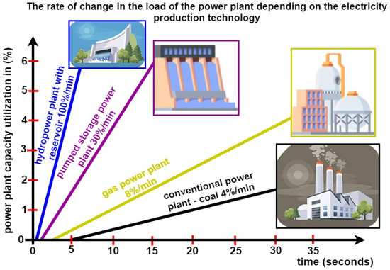
Figure 4.
Load change rate for different types of power plants operated within a PS, depending on the technology, e.g., different fuels used to generate electricity (original study).
2. Literature Review
All PS operated in specific countries worldwide should come with a certain flexibility and be characterized by a permissible minimum lower and maximum upper range of power demand adjustment over a rather short period of time [1,5,8,44]. This adjustment, or in other words, change in power demand at a given time t, is implemented within a PS always by operated power plants only. Power plants provide electricity to a PS. It can then be distributed (forwarded) to different recipients, usually consumers of varying rated capacities [6,11,20]. The power demand within a given PS can also be balanced using other available external grids, usually from neighboring countries [5,14,18,45]. The PS time of response to changing power load parameters depends on different power plant types. This enables the successful employment of various power plant types within a national power system. The time of response (time constant or inertia) to demanded power should be as short as possible. This enables covering (balancing) the power demand at a given moment in time [3,13,15,46]. The authors of the paper have encountered different proposals for technical solutions to this issue in the case of large PSs. However, the available source literature still lacks solutions for local, small-area, so-called island PSs. The authors suggest employing neural networks in a power system to predict PS demand changes and later apply these results to automatically adjust power plant capacity [8,21,28,47]. Based on the so-called artificial intelligence, it is a novel approach employed to assess load changes. It is applicable to determine power demand in small-area PSs [16,26,27,41,45].
Another important issue that has to be implemented in the PS load prediction process is the so-called continuous diagnostics process when such technical facilities are online [12,45,47]. Diagnosing technical facilities of such class is also associated with the time of response to unfitness states within a PS. An unfitness may be partial (local), e.g., failure of a single transmission line, or total (catastrophic) [17,37,41]. The latter should not occur within a PS of a given country [5,12,21,48]. In such a case, it is, e.g., a power plant’s failure that is dominant within a given PS due to its maximum output capacity [38,43,46]. It is a particularly important issue, since power facilities are always classified as SCIFs [27,33,45,47]. The process of acquiring information on the current load should be implemented in real-time, and diagnostic information should be forwarded to a PS National Dispatch [49,50,51].
The reliability of electricity supply to all consumers is also important in terms of operation. This issue must be taken into account at the engineering stage, and all national PSs must be retrofitted [27,31,33,42,52]. Currently, virtually all devices and consumers utilize electricity drawn from a PS to operate [10,25,35,40]. An unfitness within a PS (partial or total) entails tangible economic losses (e.g., stopped manufacturing process, railway or air traffic), as well as image-related losses [3,33,53,54]. Therefore, all available methods and technical solutions must be employed to improve power supply reliability within a power system, e.g., redundancy or the fail-safe principle [9,28,33,40,42].
Another extremely important parameter that characterizes all national PSs is the so-called voltage or current quality found in a given consumer’s receiving node [8,14,17,55]. This involves, e.g., content of harmonics within a PS, dips, drops, permissible grid frequency and rated voltage changes, and value of interruptions (short- and long-term) related to industrial power supply [6,9,15,44,48].
All devices and components of a PS must also exhibit sufficient resistance, strength, and susceptibility to natural and artificial interference appearing within the natural environment [44,52,56]. These include, e.g., atmospheric discharge or electromagnetic radiation sources over the entire frequency range [27,31,40,56,57]. Individual devices operating within a PS must also be fitted with anti-destruction and anti-failure elements, responding to, e.g., power grid over-voltages—e.g., varistors or fuses [17,31,42,48,58,59].
The research aim of this work is to develop a neural model using an LSTM network to forecast power demand in a small power system.
3. Power System Power Demand Changes
The local response of the system to power demand changes when this leads to a requirement to adjust the voltage at the terminals of the transformers located in switching stations (marked A and B in Figure 2) is implemented within the system at the GPZ (transformer/switching substation) level. The basic method is to employ the I&C of the AVR—Automatic Voltage Regulation. It is the I&C built into HV/HV (A—Figure 2) and HV/MV, MV/MV (B—Figure 2) transformers, implemented through changing transformer taps. The time of response to a deviation from a preset voltage level is, e.g., 120 s for the lowest difference. It is, of course, correspondingly shorter when the difference between measured and preset voltage is, respectively, higher.
A frequency drop is possible in the event of a sudden deficit in power supplied relative to the system power demand. It is a dangerous situation because it may lead to emergency generator shutdown through frequency protectors and to a cascade intensification of system failure, even resulting in a PS blackout (catastrophic failure).
The basic protection against such situations is the Automatic-Spontaneous Load Shedding (ASLS). The response time arising from the guidelines of the Power Transmission and Distribution Association (PTPiREE) is immediate. A minor delay in the case of not-yet-modernized GPZs is permissible. The ASLS I&C operation involves shutting down consumer groups (usually several MV lines) to relieve the power system. The ASLS usually has only two consumer shutdown stages. These are two different groups of all shut-down consumers—consumers within a given power grid. The second stage is implemented if the first-stage shutdown does not lead to standardizing frequency. Due to the current multitude of distributed cycle generation (consumer shutdown implementation) on MV lines, the ASLS I&C issue requires analysis and adjustments. Such actions can often be harmful due to shutting down generators coupled in an MV line string.
If there is too much generated power relative to the demand, the increased grid frequency should lead to adjustments as shown earlier. In turn, sudden changes should lead to emergency generation shutdown by over-frequency protections.
The power system in Poland is always monitored by the KDM (National Power Dispatch). Its subordinate units are
- ODM—Area Power Dispatch,
- ○
- CDM—Central Power Dispatch (central in the sense of a local distribution grid operator over a given area of the country),
- ▪
- RDM—Regional Power Dispatch.
Energy generator forecasts in terms of the electricity planned for introduction to the power system the following day are collected on a daily basis. In addition, these entities analyze weather information and its impact on generation, also based on power source, for which there is no requirement to file reports and forecasts. The volume of electricity to be drawn from the system is also determined based on historical data from previous years. KDM also takes into account the power demand in neighboring countries, coupled to common power systems. All of the information above results in a decision on the volume of electricity required from stable energy sources (e.g., coal-fired, gas-fired, and hydropower plants) and the possibility of accepting electricity from non-stable sources (wind and solar power plants). KDM forwards guidelines on the range of required electricity generation or its limitation to its subordinate units [60,61]. The information on the need to introduce restrictions is continuously monitored and adjusted, and the decisions on, e.g., shutting down/limiting power from specific sources are forwarded as late as possible, but within a time that enables their implementation without detriment to the power system and the equipment hooked up to an industrial power grid. The usual time for a PS is 1–2 h in advance.
3.1. Local Power System Power Demand Analysis
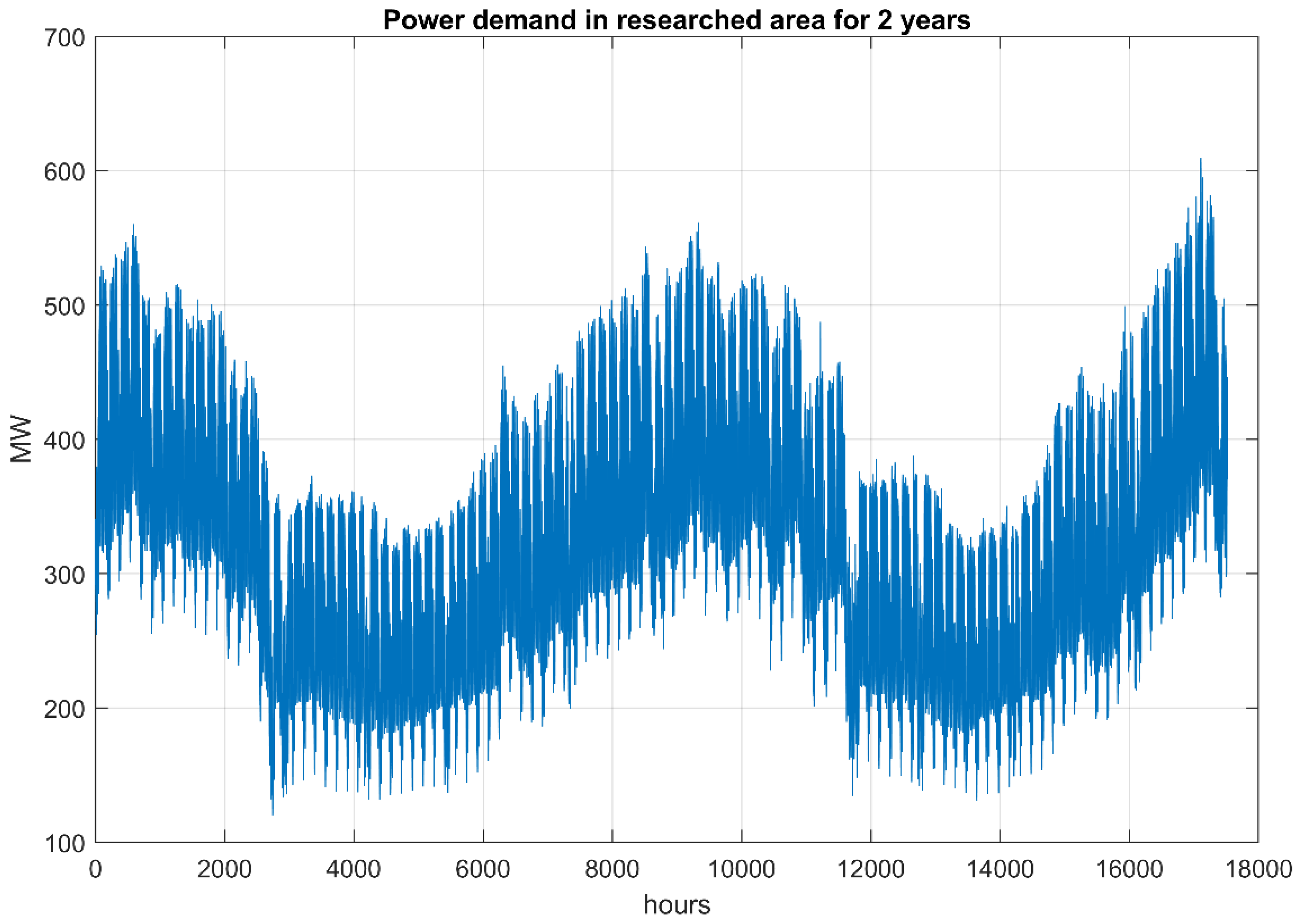
The analysis focuses on a local power system that covers the area of a large provincial city in Poland, together with its agglomeration. The power demand data related to this system was collected at a one-hour interval and covered two years. This amounts to a total of 17,520 h. The power demand time waveform is illustrated in Figure 5.

Figure 5.
Graphs showing the dynamics of electricity demand changes over a period of two years (a total of 17,520 h) in a local power system (original study).
A small power system is characterized by large power demand variability over time, as depicted in Figure 5. It is caused by its sensitivity to power supply shutdown by individual, relatively large industrial plants located within such a system and having high-capacity consumers. The fact that such sudden and significant power demand changes appear within such an isolated power grid makes forecasting related to such systems much more difficult than in the case of an entire, large system that usually covers the area of an entire country.
The most important statistical parameters of power demand within the studied area have been listed in Table 1. The range of power demand changes is very large (489.53 MW) and significantly exceeds the mean value (334.25 MW) by more than 46%. The standard deviation for these changes in the power demand was 93.47 MW, which constitutes approximately 28% of the mean value. This proves large demand variations (changes) within the studied time interval and always increases the difficulty of forecasting—predicting load changes within the t time interval in question.

Table 1.
Local power region power demand statistical parameter analysis.
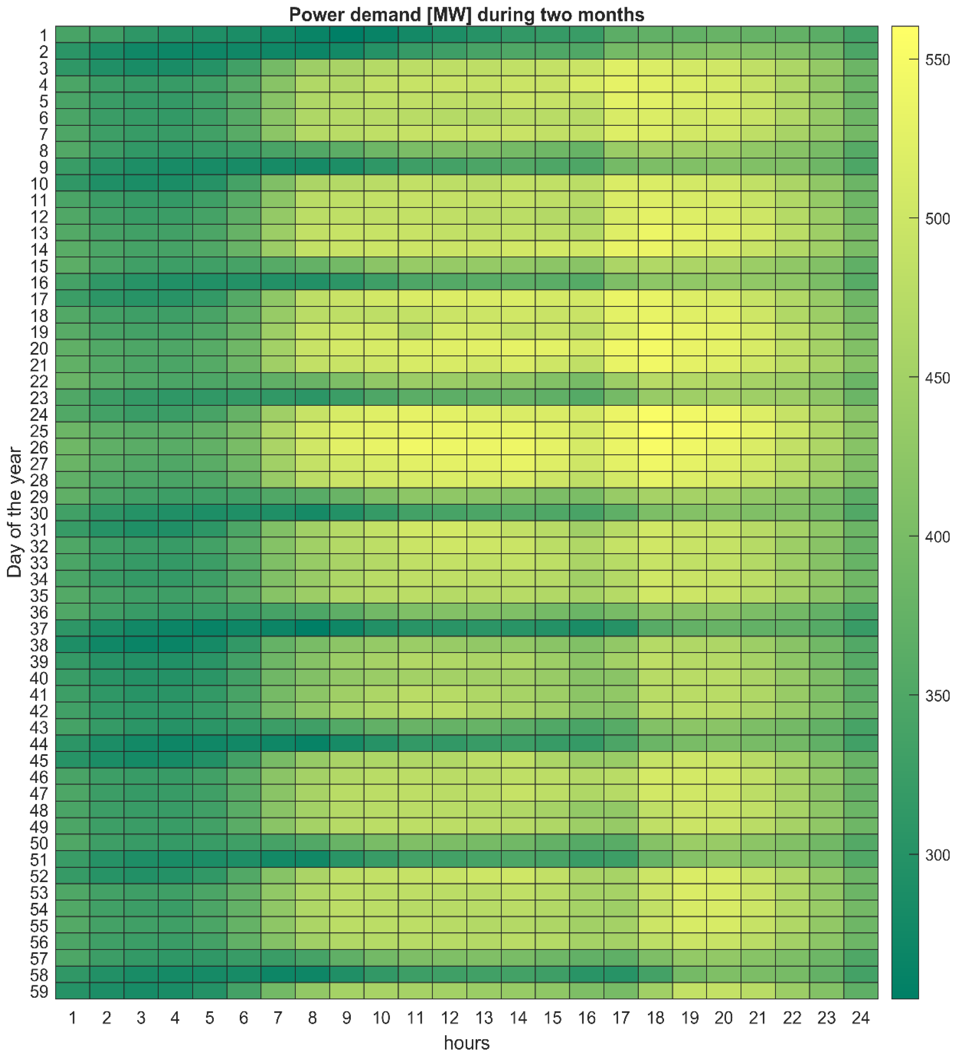
Figure 6 depicts a colored power demand map for a local power demand region over two successive months of a given year (January and February), broken down into consecutive hours of the day—on the horizontal axis.

Figure 6.
Colored power demand map showing consecutive hours for the first two months of the year, January and February, respectively—a total of 59 days. Green marks low power demand in the system, and yellow—high demand (original study).
Green marks low power demand—in the order of 300–350 MW, while yellow marks high demand—in the order of 500–550 MW (scale shown on the OY axis, to the right of the image).
3.2. Power Demand Forecasting vs. The Issue of Reducing Carbon Dioxide Atmospheric Emissions
The issue of forecasting power demand is an element of planning an entire national power system (particularly so-called own, without the help of neighboring countries, grid power balancing) that is important from technical, economic, and environmental perspectives. The stability of a given power system ensures an appropriate balance between demanded electricity and electricity supplied to a given system. When applying an accurate forecast, system operators are able to adapt the level of currently generated electricity to the current demand [62]. The solution to the problem of predicting a time series, namely, power demand within a given power region, is based on various methods. In light of the growing demand for electricity and its increasing prices, forecasting accuracy is also becoming increasingly severe in virtually all countries of the world. Over the recent years, researchers have focused their studies in this field on artificial intelligence methods, particularly neural networks (such as, e.g., MLP—Multilayer Perceptron, RBF—Radial Basis Function, and SVM—Support Vector Machine [63,64]), as well as fuzzy systems [63,64,65], evolutionary algorithms, and auto-encoders [66,67]. In addition, linear ARMAX models [66,68] are also employed for stochastic time series forecasting.
Deep neural networks, such as CNN—Convolutional Neural Networks—or LSTM—Long Short-Term Memory networks [68]—are growing in importance in relation to the power demand forecasting task. An LSTM network is structured in several layers: the input signal layer, hidden neuron feedback layer—represented by a so-called cell (Figure 7)—and an output layer. The output layer is always fed by output signals from the hidden layer [60,61].
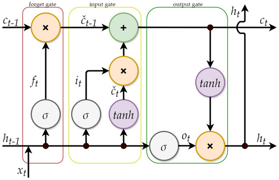
Figure 7.
Diagram of a single LSTM cell, where ft is a forget gate signal, it—input gate signal, ot—output gate signal, σ—sigmoidal activation function, tanh—hyperbolic tangent activation function, ×means multiplication, and +means adding signals (original study).
In Figure 7, the forget gate has been marked by a red frame, the input gate is marked by a yellow frame, and the output gate by a green frame. The signal flow directions have been marked by arrows. In the previous version of the drawing, not all signal flow directions were marked. In the input gate, the cell updates in the previous and present time instants have been indicated by (čt−1) and (čt), respectively.
An LSTM cell (Figure 7) processes signals over two consecutive time instants: previous (t – 1) and current (t). The xt symbol marks the input signal vector at time t. Therefore, it represents the current value of the forecast time series. The ct−1 and ct symbols mean a stored cell status at the previous and current moments, respectively. Similarly, ht−1 and ht mean hidden layer output signals at the previous and current moments, respectively. These signals are then forwarded to the output layer. The cell conducts mathematical operations as illustrated in Figure 7. They can be expressed as the L function of three input variables (ht−1, ct−1, xt) for a previous moment and two output variables (ht, ct) for a current moment, as shown through the mathematical expression No. (1).
Weight vectors are subject to adaptation within a network learning process. Learning is implemented under supervision, e.g., using an adaptive moment estimation algorithm (ADAM). After passing through the hidden layer, input data goes to the output layer. The difference between an actual and expected output value is always treated as an objective function subject to minimization. This function is then reverse-propagated by the network to calculate the gradient in the neural network weight selection optimization procedure [61].
The LSTM network was employed to predict power demand for a one-hour advance period. The number of hidden neurons was selected based on preliminary experiments in the range of 300 to 650. The best results were obtained for 465 hidden neurons. Numerical studies were implemented in the MATLAB R2023b environment. Prediction accuracy was expressed via commonly used accuracy measures, such as MAE (Mean Absolute Error)—expression No. (2),
RMSE (Root Mean Squared Error)—expression No. (3),
MAPE (Mean Absolute Percentage Error)—expression No. (4),
and Pearson’s linear correlation coefficient R—expression No. (5),
In the case of mathematical expressions No. 2, 3, 4, and 5, T(h) means an actual power demand at time h, P(h) means the demand forecast, while σ is the standard deviation. The conducted studies resulted in the following values of forecasting accuracy measures:
- MAPE = 2.7721%,
- MAE = 8.3009 MW,
- RMSE = 12.5277 MW,
- R = 0.9834.
The accuracy indices above were calculated for the entire tested range, as shown in Figure 6.
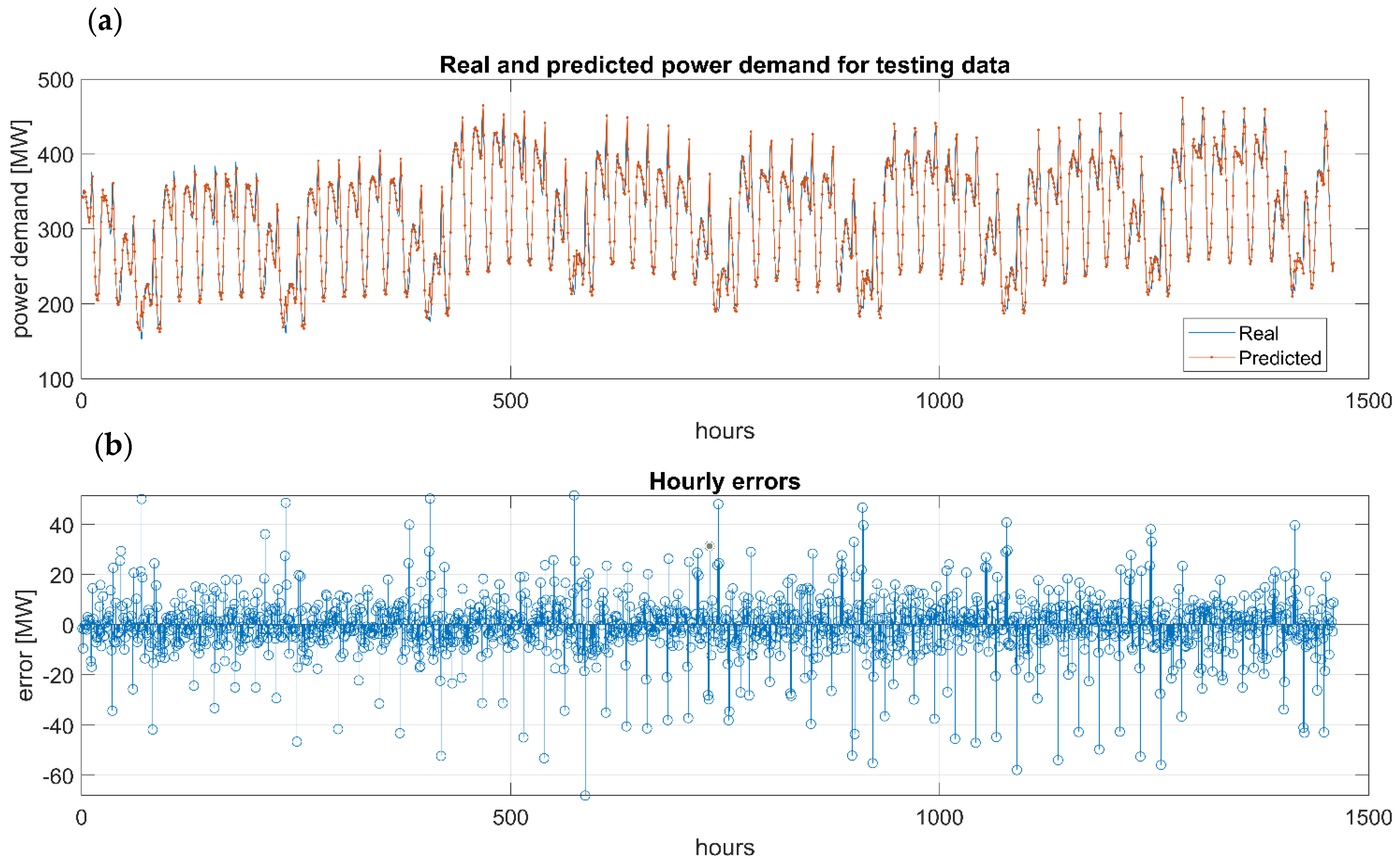
Figure 8 illustrates actual and predicted power demand for a local power region for test data not involved in learning and a period of 2 months. A good match of both curves is evident. This proves the high accuracy of the predictive method employed. Figure 8b shows marked prediction errors for consecutive power demand estimation hours.
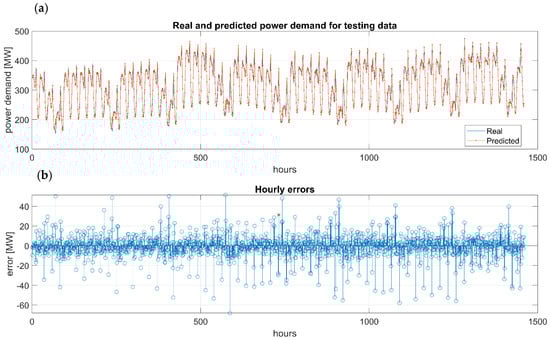
Figure 8.
(a) Actual and predicted power demand and (b) hourly errors within a local power system for a selected time interval (original study).
Input data length is at least 2 years, which amounts to a total of 17,520 h. The data has been collected at a 1 h time interval. The information on input data length is already included in Section 3.1 of the paper. Local power system power demand analysis. Approximately 80% of the input data set was allocated to learning, and the remaining 20% to testing.
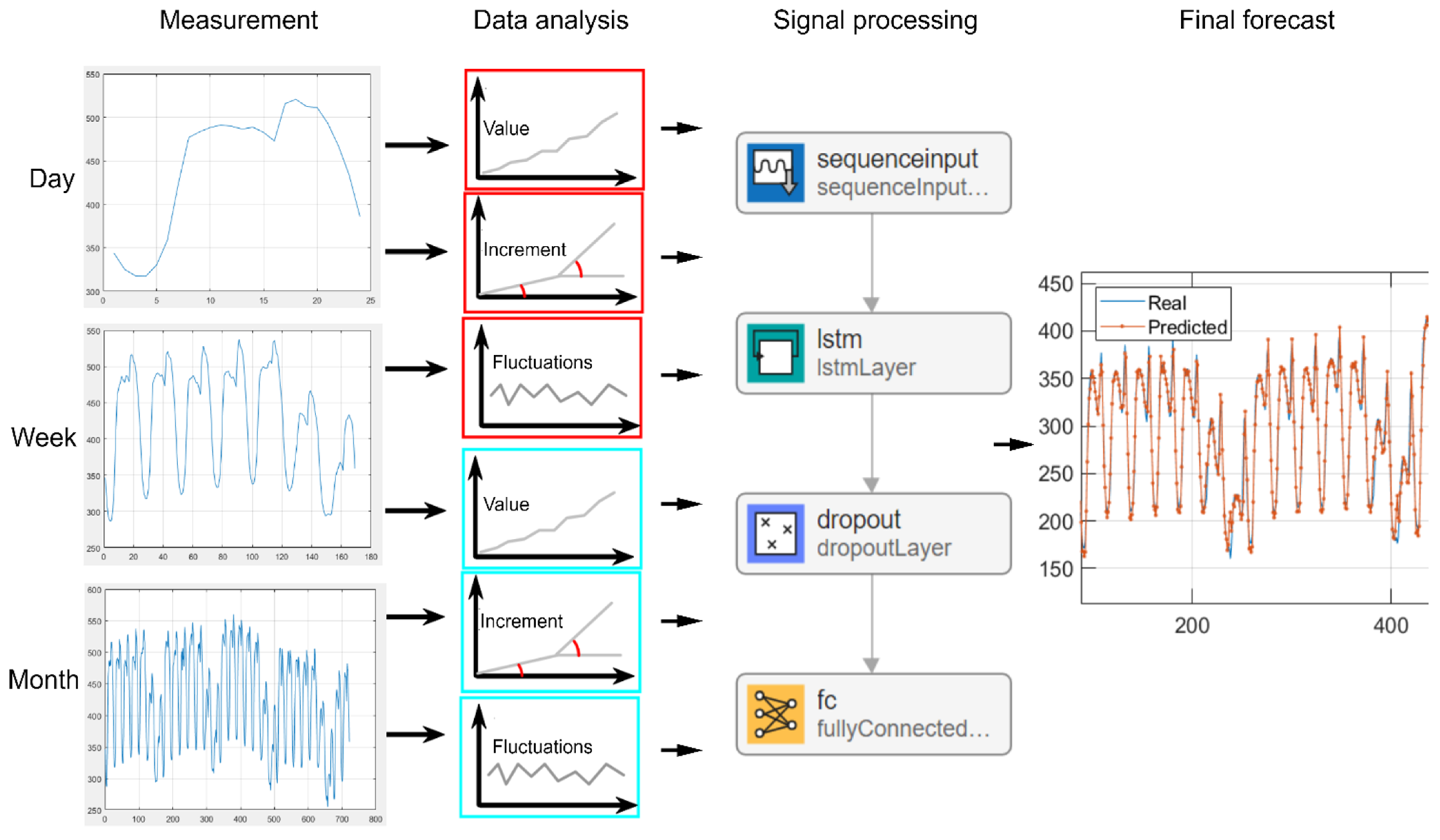
The forecasting model structure is illustrated in Figure 9 (below). Time series graphs can be found on the left: for one day, for one week, and for one month (measurement). The next block is input data analysis that includes data standardization as per the formula:
where: xj—standardized value of demand at time j; rj—true demand value prior to standardization at time j; m—mean demand value within the studied time interval; σ—standard deviation within the studied time interval.
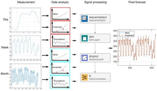
Figure 9.
Scheme of the proposed forecasting model. In Signal processing column: the first one is sequenceInputLayer, the fourth one is fullyConnectedLayer.
Next, the authors presented a diagram of the employed LSTM network (signal processing). The sequence Input Layer prepares data for forecasting. It involves determining the number of features subject to forecasting. It is followed by the IstmLayer, where the number of hidden neurons is specified. Next comes the dropout layer, which is responsible for regularization with a preset probability. The fully connected layer multiplies inputs through a weight matrix and adds a bias vector to it. The final forecast is the outcome of a forecasting team comprising 5 trained LSTM networks. The operations of the LSTM network are repeated 5 times, and the end result (final forecast) is an arithmetic mean for the entire team—Table 2. The application of an artificial neural network to forecast electricity demand in small power systems enables automatic learning based on current change observations. This also includes automatic generalization of knowledge gained throughout the entire process of using such software in the power utilities’ local power distribution center. These processes are often not properly implemented, particularly in small power regions.
Table 2.
Parameters of the proposed forecasting model—search space for the optimal and selected parameter.
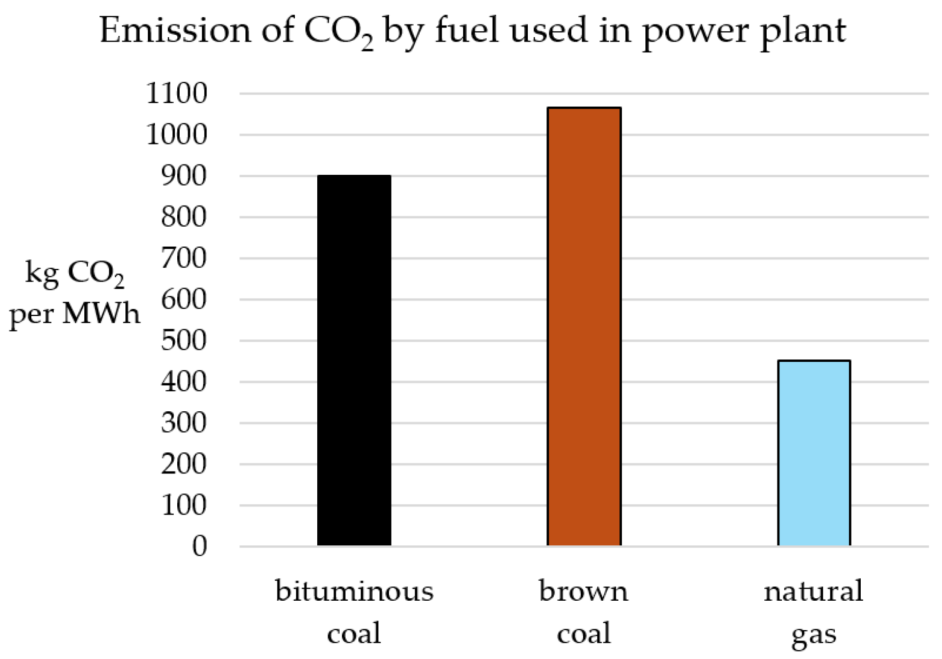
Figure 10 depicts a graph that illustrates the amount of carbon dioxide (CO2) emitted to the atmosphere per one-megawatt hour (MWh) of electricity generated by a power plant, taking into account the fuel used by conventional power plants of a given type.

Figure 10.
Atmospheric carbon dioxide (CO2) emissions in kg/MWh of generated electricity, broken down into different types of fuels used in conventional power plants (hard coal, lignite, natural gas) (original study).
The highest CO2 emission per 1 MWh of electricity generated is recorded in the case of lignite coal and amounts to 1065 kg CO2/MWh. In turn, this parameter in hard coal-fired power plants is 900 kg CO2/MWh, and in the case of natural gas-fired power plants, 450 kg CO2/MWh.
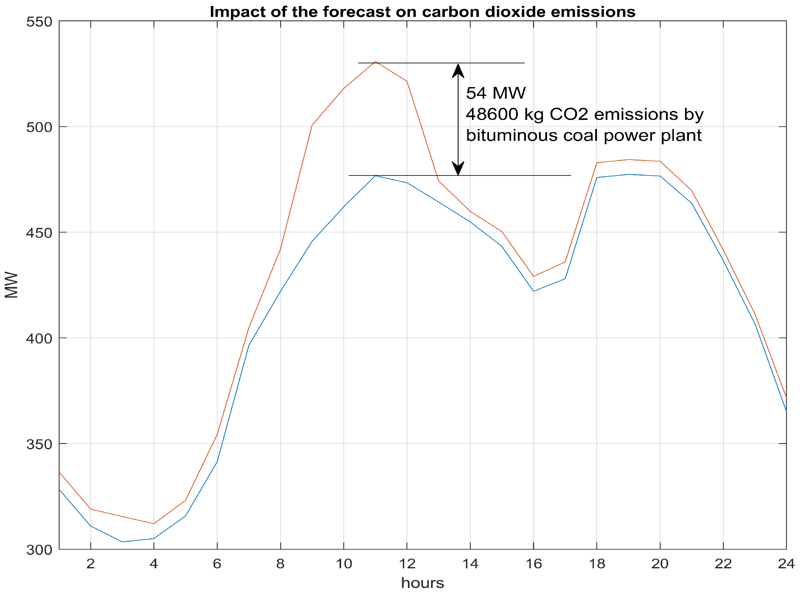
According to the data in [54,66,69], 46.9% of the electricity in Poland was generated in hard coal-fired power plants, 22.5%—in lignite-fired power plants, and 13.2%—in natural gas power plants. Therefore, the three fuel types referred to account for 82.6% of electricity generation in Poland (as of 10 February 2025). Figure 11 illustrates the impact of an accurate forecast on the reduction in the emissions of a selected greenhouse gas (CO2) upon the application of a coal-fired power plant power demand prediction developed by an artificial neural network. Prediction enables electricity generation to adapt to the current demand. This leads to savings, both in terms of generating the electricity itself and losses during transmission over large distances (power plant—transformer station—switching stations—consumer—Figure 2), and therefore, in the fuel consumed to generate 1 kWh in a power system.
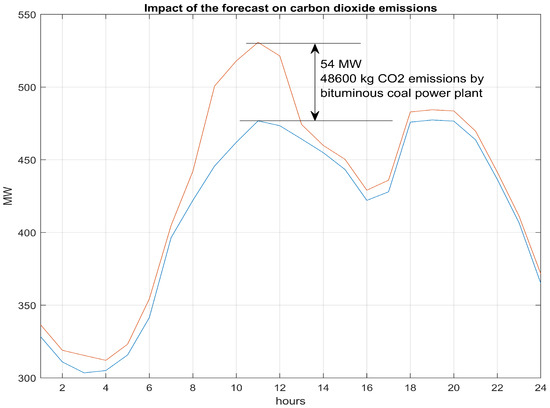
Figure 11.
Impact of employing power demand forecasts on reduced carbon dioxide atmospheric emissions—hard coal-fired power plant (original study).
This also means a significant reduction in the production and emission of greenhouse gases into the atmosphere. Limiting the level of generated power by, e.g., 54 MW in one hour leads to reduced CO2 emissions by as much as 48,600 kg in a conventional, hard coal-fired power plant. In a lignite-fired power plant, where unit emissions were even higher, this value is 57,510 kg CO2, and 24,300 kg CO2 for a gas-fired power plant. Figure 11 illustrates the impact of employing power demand prediction on reduced carbon dioxide atmospheric emissions in the case of coal-fired power plants in a PS.
Figure 11 is aimed at demonstrating how information originating from a load forecast for the following hour (during a morning peak) may impact reducing atmospheric CO2 emissions of a coal-fired power plant. Reducing generated power by, e.g., 54 MW, possibly owing to next-hour demand information, enables reducing CO2 emissions by 48,600 kg. Figure 11 is aimed at illustrating an example of a situation wherein knowing power demand in the following hours, during a morning peak, enables reducing the atmospheric emissions of CO2 generated by a coal-fired power plant.
The developed method triggers industrial energy storage as well as hydropower plants located on waterways in northern Poland. Industrial energy storage is often installed in plants with extensive high-capacity photovoltaic systems. The aforementioned adjustments (increased power demand) are implemented in practice without time delay. The introduction of an additional power supply to a power system is immediately visible on power demand graphs received in real time. Of course, employing other technical solutions to increase power in a system—e.g.; increasing the capacity of a CHP with an additional power generator—requires the existence of feedback—i.e.; information on the system’s response to increased power. The authors are currently implementing such research in relation to another power system, thus creating an opportunity for comparison—e.g.; control quality (e.g., power system’s response time to forced actions—power increase). Companies (electricity distributors) within a given area do not provide information since the domestic power market is currently experiencing fierce competition.
4. Conclusions
The prediction and analysis of power demand for small power grids conducted using artificial intelligence (using a deep neural network, LSTM, in this case) clearly confirmed that this might become one of the ways to limit carbon dioxide atmospheric emissions. An analysis of the power demand issue and the research that was conducted indicated that such an application of a neural network is a good tool for forecasting short-term demand in a local power system. Knowledge of the power demanded within a power system over the next hour allows an operator to increase or reduce electricity generation, depending on the needs of the entire power system. This ensures reliable operation and balancing of the entire power system—in this case; for small power grids. Forecasting power demand in a local power system significantly contributes to reducing greenhouse gas atmospheric emissions. Employing accurate forecasts is important in small power systems, which experience relatively large changes (sudden surges) in the power demand throughout the day. Conventional power plants (that use hard coal, lignite, or natural gas as fuel), where the rate of electricity generation changes the least (around 4%/min.), require knowledge of forecast demand well in advance—significantly faster than; e.g., hydro or pumped hydropower plants. This is caused by the fact that they are unable to reduce generated power over a rather short period of time and, hence, cut the atmospheric emissions of harmful greenhouse gases, which are subject to specific emission limits in individual EU countries. Reducing electricity demand within an industrial power system by, e.g., as little as 54 MW in just one hour of its operation leads to CO2 emissions reduced by as much as 48,600 kg in a conventional power plant with hard coal as its fuel. It is different in the case of a power plant with lignite or natural gas as its fuel.
In the former case, a lignite-fired power plant, unit CO2 emissions will be many times higher. This value amounts to 57,510 kg CO2. And respectively, 24,300 kg CO2 for a gas-fired power plant.
Figure 10 is a presentation of the authors’ analysis of the impact of employing power demand prediction in small power grids on reduced carbon dioxide atmospheric emissions in the case of coal-fired power plants in a PS.
The authors of the article employed a neural network for computer predictions of load within a power grid, without previous mathematical formalization of the state of the issue. Using a neural network to predict load changes in power grids also makes it possible not to reference any theoretical assumptions in relation to the issue being solved. The availability of power grid load results, particularly their analysis in individual power plants supplying specific regions, is low. The application of a neural network and its capability to learn based on a current change in the power load enables automatic generalization of the knowledge gained throughout the entire process of using such software within a power distribution center of power plants. In their preliminary research, the authors of the article have referred to only one country, i.e., Poland. They based their research on an ‘island’ power system located north of the country, which experiences significant distances to the nearest power plants. A crucial research problem when conducting this task was also obtaining power demand data. The approach to this issue of companies supplying electricity to consumers in this area differs from company to company. Rather, they are competitors and do not always intend to share the data they consider confidential. However, while continuing to work on this problem, the authors are trying to interest the nearest countries and neighbors in this research topic.
Author Contributions
Conceptualization, J.P., T.C. and S.D.; methodology, J.P., T.C. and S.D.; validation, J.P., M.S., T.C. and S.D.; formal analysis, S.D., J.P. and T.C.; investigation, J.P., M.S., T.C. and S.D.; resources, M.S., T.C. and S.D.; data curation, J.P., M.S., T.C. and S.D.; writing—original draft preparation, J.P., M.S., T.C. and S.D.; writing—review and editing, J.P., M.S. and T.C.; supervision, J.P., T.C. and S.D.; project administration, J.P., M.S., T.C. and S.D.; funding acquisition, J.P., M.S., T.C. and S.D. All authors have read and agreed to the published version of the manuscript.
Funding
This work was financed/co-financed by the Military University of Technology under research project UGB/22-060/2025/WAT, “Research on the use of modern measurement techniques, digital signal processing, and artificial intelligence methods in monitoring and security systems”.
Institutional Review Board Statement
Not applicable.
Informed Consent Statement
Not applicable.
Data Availability Statement
The data presented in this study are available on request from the corresponding author.
Conflicts of Interest
The authors declare no conflicts of interest.
Abbreviations
The following symbols and acronyms are used in this manuscript:
| PS | Power System |
| PL | Power Lines |
| SS | Switching Stations |
| SCIF | State Critical Infrastructure Facilities |
| NPS | National Power System |
| KDM | National Power Dispatch |
| LPS | Local Power System |
| PTPiREE | Polish Power Transmission and Distribution Association |
| HV/MV | High voltage/medium voltage |
| ULS | Underfrequency Load Shedding |
| GPZ | Transformer/Switching Substation |
| MLP | Multilayer Perceptron |
| RBF | Radial Basis Function |
| SVM | Support Vector Machine |
| ARMAX | AutoRegressive Moving Average with eXogenous input |
| CNN | Convolutional Neural Network |
| LSTM | Long Short-Term Memory |
| ADAM | Adaptive Moment Estimation |
| MAE | Mean Absolute Error |
| RMSE | Root Mean Squared Error |
| MAPE | Mean Absolute Percentage Error |
| R | Pearson correlation coefficient |
| ASLS | Automatic-Spontaneous Load Shedding |
| ODM | Area Power Dispatch |
| CPD | Central Power Dispatch |
| RDM | Regional Power Dispatch |
References
- Lund, H.; Thellufsen, J.Z.; Østergaard, P.A.; Sorknæs, P.; Skov, I.R.; Mathiesen, B.V. EnergyPLAN—Advanced analysis of smart energy systems. Smart Energy 2021, 1, 100007. [Google Scholar] [CrossRef]
- Barnes, T.; Shivakumar, A.; Brinkerink, M.; Niet, T. OSeMOSYS Global, an open-source, open data global electricity system model generator. Sci. Data 2022, 9, 623. [Google Scholar] [CrossRef] [PubMed]
- Esmaeili Aliabadi, D.; Wulff, N.; Jordan, M.; Cyffka, K.F.; Millinger, M. Soft-coupling energy and power system models to analyze pathways toward a de-fossilized German transport sector. In Operations Research Proceedings 2022; Lecture Notes in Operations Research; Springer: Berlin/Heidelberg, Germany, 2023. [Google Scholar] [CrossRef]
- Caban, D.; Walkowiak, T. Dependability analysis of hierarchically composed system-of-systems. In Proceedings of the Thirteenth International Conference on Dependability and Complex Systems DepCoS-RELCOMEX, Brunów, Poland, 2–6 July 2018; Springer: Cham, Switzerland, 2019; pp. 113–120. [Google Scholar] [CrossRef]
- Olivares, D.E.; Mehrizi-Sani, A.; Etemadi, A.H.; Cañizares, C.A.; Iravani, R.; Kazerani, M.; Hajimiragha, A.H.; Gomis-Bellmunt, O.; Saeedifard, M.; Palma-Behnke, R.; et al. Trends in Microgrid Control. IEEE Trans. Smart Grid 2014, 5, 1905–1919. [Google Scholar] [CrossRef]
- Hassan, S.U.; Abi, Z.U.; Izhar, T. Advanced control techniques for micro-grids power quality improvement. In Proceedings of the 2017 Asian Conference on Energy, Power and Transportation Electrification (ACEPT), Singapore, 24–26 October 2017; pp. 1–6. [Google Scholar] [CrossRef]
- Łukasiak, J.; Rosiński, A.; Wiśnios, M. The Issue of Evaluating the Effectiveness of Miniature Safety Fuses as Anti-Damage Systems. Energies 2022, 15, 4013. [Google Scholar] [CrossRef]
- Skuza, A.; Ziemianek, S.; Suproniuk, M. Power System Division—Certain Issues Associated with Shaping Commutation Strategies in Power Substations. Energies 2022, 15, 7293. [Google Scholar] [CrossRef]
- Adhikari, S.; Li, F.; Li, H. P-Q and P-V Control of Photovoltaic Generators in Distribution Systems. IEEE Trans. Smart Grid 2015, 6, 2929–2941. [Google Scholar] [CrossRef]
- Singh, M.; Khadkikar, V.; Chandra, A.; Varma, R.K. Grid Interconnection of Renewable Energy Sources at the Distribution Level With Power-Quality Improvement Features. IEEE Trans. Power Deliv. 2011, 26, 307–315. [Google Scholar] [CrossRef]
- Naderipour, A.; Abdul-Malek, Z.; Afrouzi, H.N.; Ramachandaramurthy, V.K.; Guerrero, J.M. A Novel Compensation Current Control Method for Grid-Connected PV Inverter to Improve Power Quality in Micro-Grid. In Proceedings of the 2018 IEEE PES Asia-Pacific Power and Energy Engineering Conference (APPEEC), Kota Kinabalu, Malaysia, 7–10 October 2018; pp. 143–148. [Google Scholar] [CrossRef]
- Kaur, G.; Associate, A.P.; Rao, K.U. Design and Implementation of Hybrid Microgrid in MATLAB for Fault Current Analysis in Different Modes of Microgrid Operations. In Proceedings of the 2019 3rd International Conference on Recent Developments in Control, Automation & Power Engineering (RDCAPE), Noida, India, 10–11 October 2019; pp. 368–372. [Google Scholar] [CrossRef]
- Salmeron, P.; Herrera, R.S.; Vazquez, J.R. Mapping matrices against vectorial frame in the instantaneous reactive power compensation. IET Electr. Power Appl. 2007, 1, 727–736. [Google Scholar] [CrossRef]
- Li, Y.; Guldenmund, F.W. Safety management systems: A broad overview of the literature. Saf. Sci. 2018, 103, 94–123. [Google Scholar] [CrossRef]
- Chiang, S.Y.; Kan, Y.C.; Chen, Y.S.; Tu, Y.C.; Lin, H.C. Fuzzy computing model of activity recognition on WSN movement data for ubiquitous healthcare measurement. Sensors 2016, 16, 2053. [Google Scholar] [CrossRef]
- Siergiejczyk, M.; Paś, J.; Rosiński, A. Evaluation of Safety of Highway CCTV System’s Maintenance Process. In Telematics—Support for Transport. TST 2014. Communications in Computer and Information Science; Mikulski, J., Ed.; Springer: Berlin/Heidelberg, Germany, 2014; Volume 471, pp. 69–79. [Google Scholar] [CrossRef]
- Dziula, P.; Paś, J. Low Frequency Electromagnetic Interferences Impact on Transport Security Systems Used in Wide Transport Areas. TransNav Int. J. Mar. Navig. Saf. Sea Transp. 2018, 12, 251–258. [Google Scholar] [CrossRef]
- Shah, A.U.A.; Christian, R.; Kim, J.; Kim, J.; Park, J.; Kang, H.G. Dynamic Probabilistic Risk Assessment Based Response Surface Approach for FLEX and Accident Tolerant Fuels for Medium Break LOCA Spectrum. Energies 2021, 14, 2490. [Google Scholar] [CrossRef]
- Chen, C.Y.; Liu, H.L.; Xiao, Y.; Zhu, F.G.; Ding, L.; Yang, F.W. Power generation scheduling for a hydro-wind-solar hybrid system: A systematic survey and prospect. Energies 2022, 15, 8747. [Google Scholar] [CrossRef]
- Yu, L.; Wu, X.F.; Zhou, Z.H. Multi-objective optimal operation of cascade hydropower plants considering ecological flow under different ecological conditions. J. Hydrol. 2021, 601, 126599. [Google Scholar] [CrossRef]
- Farahmand, H.; Jaehnert, S.; Aigner, T.; Huertas-Hernando, D. Nordic hydropower flexibility and transmission expansion to support integration of North European wind power. Wind Energy 2015, 18, 1075–1103. [Google Scholar] [CrossRef]
- Naghdalian, S.; Amraee, T.; Kamali, S.; Capitanescu, F. Stochastic network constrained unit commitment to determine flexible ramp reserve for handling wind power and demand uncertainties. IEEE Trans. Ind. Inform. 2020, 16, 4580–4591. [Google Scholar] [CrossRef]
- Süsser, D.; Gaschnig, H.; Ceglarz, A.; Stavrakas, V.; Flamos, A.; Lilliestam, J. Better suited or just more complex? On the fit between user needs and modeller-driven improvements of energy system models. Energy 2022, 239, 121909. [Google Scholar] [CrossRef]
- Oberle, S.; Elsland, R. Are open access models able to assess today’s energy scenarios? Energy Strategy Rev. 2019, 26, 100396. [Google Scholar] [CrossRef]
- Siergiejczyk, M.; Paś, J.; Rosiński, A. Modeling of process of exploitation of transport telematics systems with regard to electro-magnetic interferences. In Proceedings of the TOOLS OF TRANSPORT TELEMATICS, 15th International Conference on Transport Systems Telematics (TST), Wrocław, Poland, 15–17 April 2015; Volume 531, pp. 99–107. [Google Scholar] [CrossRef]
- Moezzi, M.; Janda, K.B.; Rotmann, S. Using stories, narratives, and storytelling in energy and climate change research. Energy Res. Soc. Sci. 2017, 31, 1–10. [Google Scholar] [CrossRef]
- Wiśnios, M.; Tatko, S.; Mazur, M.; Paś, J.; Łukasiak, J.M.; Klimczak, T. Identifying Characteristic Fire Properties with Stationary and Non-Stationary Fire Alarm Systems. Sensors 2024, 24, 2772. [Google Scholar] [CrossRef]
- Nitsch, F.; Schimeczek, C.; Nienhaus, K.; Frey, U.; Sperber, E.; Sarfarazi, S.; Kochems, J.; El Ghazi, A.A. AMIRIS-The Open Agent-based Market Model: How to get involved and profit from our model. In Proceedings of the Openmod Workshop, Laxenburg, Austria, 22–24 March 2023. [Google Scholar]
- Kwasiborska, A.; Skorupski, J. Assessment of the Method of Merging Landing Aircraft Streams in the Context of Fuel Consumption in the Airspace. Sustainability 2021, 13, 12859. [Google Scholar] [CrossRef]
- Antosz, K.; Machado, J.; Mazurkiewicz, D.; Antonelli, D.; Soares, F. Systems Engineering: Availability and Reliability. Appl. Sci. 2022, 12, 2504. [Google Scholar] [CrossRef]
- Jakubowski, K.; Paś, J.; Duer, S.; Bugaj, J. Operational Analysis of Fire Alarm Systems with a Focused, Dispersed and Mixed Structure in Critical Infrastructure Buildings. Energies 2021, 14, 7893. [Google Scholar] [CrossRef]
- Vinogradov, A.; Bolshev, V.; Vinogradova, A.; Jasiński, M.; Sikorski, T.; Leonowicz, Z.; Goňo, R.; Jasińska, E. Analysis of the power supply restoration time after failures in power transmission lines. Energies 2020, 13, 2736. [Google Scholar] [CrossRef]
- Sterniczuk, D.; Zaklika, W.; Kozłowski, M. Identification Tests of Modern Vehicles’ Electromagnetic Environment as Part of the Assessment of Their Functional Safety. Sensors 2025, 25, 7. [Google Scholar] [CrossRef]
- Soszyńska-Budny, J. General approach to critical infrastructure safety modelling. In Safety Analysis of Critical Infrastructure. Lecture Notes in Intelligent Transportation and Infrastructure; Springer: Cham, Switzerland, 2021. [Google Scholar]
- Ruddle, A.R.; Martin, A.J.M. Adapting automotive EMC to meet the needs of the 21st century. IEEE Electromagn. Compat. Mag. 2019, 8, 75–85. [Google Scholar] [CrossRef]
- Stawowy, M.; Rosiński, A.; Siergiejczyk, M.; Perlicki, K. Quality and Reliability-Exploitation Modeling of Power Supply Systems. Energies 2021, 14, 2727. [Google Scholar] [CrossRef]
- Łukasiak, J.; Rosiński, A.; Wiśnios, M. The Impact of Temperature of the Tripping Thresholds of Intrusion Detection System Detection Circuits. Energies 2021, 14, 6851. [Google Scholar] [CrossRef]
- Slowak, P.; Kaniewski, P. Stratified Particle Filter Monocular SLAM. Remote Sens. 2021, 13, 3233. [Google Scholar] [CrossRef]
- Pas, J.; Klimczak, T.; Rosinski, A.; Stawowy, M. The analysis of the operational process of a complex fire alarm system used in transport facilities. Build. Simul. 2022, 15, 615–629. [Google Scholar] [CrossRef]
- Paś, J.; Rosiński, A.; Białek, K. A reliability-exploitation analysis of a static converter taking into account electromagnetic interference. Transp. Telecommun. 2021, 22, 217–229. [Google Scholar] [CrossRef]
- Paś, J.; Rosiński, A.; Wetoszka, P.; Białek, K.; Klimczak, T.; Siergiejczyk, M. Assessment of the Impact of Emitted Radiated Interference Generated by a Selected Rail Traction Unit on the Operating Process of Trackside Video Monitoring Systems. Electronics 2022, 11, 2554. [Google Scholar] [CrossRef]
- Rosiński, A.; Paś, J.; Białek, K. A reliability-operational analysis of a track-side CCTV cabinet taking into account interference, Bulletin of the Polish Academy of sciences. Tech. Sci. 2021, 69, 1–11. [Google Scholar] [CrossRef]
- Pham, H. Safety and RiskModeling and its Applications; Springer Series in Reliability Engineering; Springer: London, UK, 2011; p. 125. [Google Scholar]
- Saleh, J.H.; Haga, R.A.; Favarò, F.M.; Bakolas, E. Texas City refinery accident: Case study in breakdown of defense-in-depth and violation of the safety—Diagnosability principle in design. Eng. Fail. Anal. 2014, 36, 121–133. [Google Scholar] [CrossRef]
- Duer, S.; Rokosz, K.; Zajkowski, K.; Bernatowicz, D.; Ostrowski, A.; Woźniak, M.; Iqbal, A. Intelligent Systems Supporting the Use of Energy Devices and Other Complex Technical Objects: Modeling, Testing, and Analysis of Their Reliability in the Operating Process. Energies 2022, 15, 6414. [Google Scholar] [CrossRef]
- Oszczypała, M.; Ziółkowski, J.; Małachowski, J. Analysis of Light Utility Vehicle Readiness in Military Transportation Systems Using Markov and Semi-Markov Processes. Energies 2022, 15, 5062. [Google Scholar] [CrossRef]
- Duer, S.; Zajkowski, K.; Harničárová, M.; Charun, H.; Bernatowicz, D. Examination of Multivalent Diagnoses Developed by a Diagnostic Program with an Artificial Neural Network for Devices in the Electric Hybrid Power Supply System “House on Water”. Energies 2021, 14, 2153. [Google Scholar] [CrossRef]
- Veit, S.; Steiner, F. Defect Trends in Fire Alarm Systems: A Basis for Risk-Based Inspection (RBI) Approaches. Safety 2024, 10, 95. [Google Scholar] [CrossRef]
- Duer, S. Diagnostic system for the diagnosis of a reparable technical object, with the use of an artificial neural network of RBF type. Neural Comput. Appl. 2010, 19, 691–700. [Google Scholar] [CrossRef]
- Kaniewski, P. Extended Kalman Filter with Reduced Computational Demands for Systems with Non-Linear Measurement Models. Sensors 2020, 20, 1584. [Google Scholar] [CrossRef]
- Gajjar, S.; Palazoglu, A. A data-driven multidimensional visualization technique for process fault detection and diagnosis. Chemom. Intell. Lab. Syst. 2016, 154, 122–136. [Google Scholar] [CrossRef]
- Kang, Y.; Duan, B.; Zhou, Z.; Shang, Y.; Zhang, C. A multi-fault diagnostic method based on an interleaved voltage measurement topology for series connected battery packs. J. Power Sources 2019, 417, 132–144. [Google Scholar] [CrossRef]
- Stawowy, M.; Perlicki, K.; Sumiła, M. Comparison of uncertainty multilevel models to ensure ITS services. In Safety and Reliability: Theory and Applications, Proceedings of the European Safety and Reliability Conference ESREL 2017, Portoroz, Slovenia, 18–22 June 2017; Cepin, M., Bris, R., Eds.; CRC Press/Balkema: London, UK, 2017; pp. 2647–2652. [Google Scholar]
- Szczupak, P.; Kossowski, T.; Szostek, K.; Szczupak, M. Tests of pulse interference from lightning discharges occurring in unmanned aerial vehicle housings made of carbon fibers. Eksploat. I Niezawodn.—Maint. Reliability 2024, 27, 193984. [Google Scholar] [CrossRef]
- Sadeghi, B.; Westerlund, P.; Giri, M.; Bollen, M. Analysis of the Measurements of the Radiated Emission from 9 kHz to 150 kHz from Electric Railways. Energies 2024, 17, 4951. [Google Scholar] [CrossRef]
- Xu, Z.; Lei, C.; Yan, F. Electromagnetic safety evaluation of Advanced Driving Assistance System in the anechoic chamber. In Proceedings of the 2022 Asia-Pacific International Symposium on Electromagnetic Compatibility (APEMC), Beijing, China, 8–11 May 2022; pp. 119–122. [Google Scholar] [CrossRef]
- Sabat, W.; Klepacki, D.; Kamuda, K.; Kuryło, K.; Jankowski-Mihułowicz, P. Estimation of the Immunity of an AC/DC Converter of an LED Lamp to a Standardized Electromagnetic Surge. Electronics 2024, 13, 4607. [Google Scholar] [CrossRef]
- Burdzik, R. Application of vibration signals as independent and alternative information channels to support the reliability of positioning and prediction systems for transport means movement. Eksploat. I Niezawodn.—Maint. Reliability 2025, 27, 196929. [Google Scholar] [CrossRef]
- Duer, S. Examination of the reliability of a technical object after its regeneration in a maintenance system with an artificial neural network. Neural Comput. Appl. 2012, 21, 523–534. [Google Scholar] [CrossRef]
- Osowski, S.; Szmurlo, R.; Siwek, K.; Ciechulski, T. Neural Approaches to Short-Time Load Forecasting in Power Systems—A Comparative Study. Energies 2022, 15, 3265. [Google Scholar] [CrossRef]
- Ciechulski, T.; Osowski, S. High Precision LSTM Model for Short-Time Load Forecasting in Power Systems. Energies 2021, 14, 2983. [Google Scholar] [CrossRef]
- Ciechulski, T.; Osowski, S. Deep Learning Approach to Power Demand Forecasting in Polish Power System. Energies 2020, 13, 6154. [Google Scholar] [CrossRef]
- Ciechulski, T.; Osowski, S. The method of 24-hour load forecasting with application of fuzzy sets and C-means algorithm. Przegląd Elektrotechniczny 2019, 10, 185–189. [Google Scholar] [CrossRef]
- Ciechulski, T.; Osowski, S. The neural method applied for 24-hour load forecasting for the next day in National Power System in Poland. Przegląd Elektrotechniczny 2018, 9, 108–112. [Google Scholar] [CrossRef]
- Ceschini, A.; Rosato, A.; Panella, M. Design of an LSTM cell on a quantum hardware. IEEE Trans. Circuits Syst. 2022, 69, 1822–1826. [Google Scholar] [CrossRef]
- Herui, C.; Xu, P.; Yupei, M. Electric Load Forecast Using Combined Models with HP Filter-SARIMA and ARMAX Optimized by Regression Analysis Algorithm. Math. Probl. Eng. 2015, 2015, 386925. [Google Scholar] [CrossRef]
- Liu, P.; Zheng, P.; Chen, Z. Deep Learning with Stacked Denoising Auto-Encoder for Short-Term Electric Load Forecasting. Energies 2019, 12, 2445. [Google Scholar] [CrossRef]
- Hochreiter, S.; Schmidhuber, J. Long short-term memory. Neural Comput. 1997, 9, 1735–1780. [Google Scholar] [CrossRef]
- Structure and Production of Electricity in Poland. Available online: https://www.cire.pl/strony/struktura-i-produkcja-energii-elektrycznej-w-polsce (accessed on 11 February 2025).


Disclaimer/Publisher’s Note: The statements, opinions and data contained in all publications are solely those of the individual author(s) and contributor(s) and not of MDPI and/or the editor(s). MDPI and/or the editor(s) disclaim responsibility for any injury to people or property resulting from any ideas, methods, instructions or products referred to in the content. |
© 2025 by the authors. Licensee MDPI, Basel, Switzerland. This article is an open access article distributed under the terms and conditions of the Creative Commons Attribution (CC BY) license (https://creativecommons.org/licenses/by/4.0/).