Abstract
With the rapid development of industrial internet, blockchain, and other new-generation information technology, the shared manufacturing model provides a new way to address the problems of low resource utilization of the traditional manufacturing industry and serious duplication of construction through the mechanism of collaborative resource sharing. Concurrently, to meet the requirements of sustainable development, manufacturing enterprises need to balance economic efficiency with production efficiency in their production practices. This study investigates an identical parallel machine offline scheduling problem with rental costs and shared service costs of shared machines. In machine renting, manufacturers with a certain number of identical parallel machines will incur fixed rental costs, unit variable rental costs, and shared service costs when renting the shared machines. The objective is to minimize the sum of the makespan and total sharing costs. To address this problem, an integer linear programming model is established, and several properties of the optimal solution are provided. A heuristic algorithm based on the number of rented machines is designed. Finally, numerical simulation experiments are conducted to compare the proposed heuristic algorithm with a genetic algorithm and the longest processing time (LPT) rule. The results demonstrate the effectiveness of the proposed heuristic algorithm in terms of calculation accuracy and efficiency. Additionally, the experimental findings reveal that the renting and scheduling results of the machines are influenced by various factors, such as the manufacturer’s production conditions, the characteristics of the jobs to be processed, production objectives, rental costs, and shared service costs.
1. Introduction
Shared manufacturing, relying on new infrastructures such as 5G, artificial intelligence, the industrial internet, and the internet of things, has quietly emerged and shown a booming development [1,2]. Shared manufacturing is the reuse of idle production capacity, which can optimize resource allocation, break information asymmetry, reduce manufacturing costs, expand effective supply, and enhance manufacturing service capabilities and levels [3], in line with the concept of sustainable development. As a result, shared manufacturing has become one of the key themes driving the high-quality and sustainable development of the manufacturing industry, aligning with the trend towards intelligent, efficient, and service-oriented economic development.
Under the impetus of development demands and policy support, many Chinese enterprises have achieved fruitful practices in implementing sharing systems. For example, the “Oscar COSMOPlat” has connected 900,000 enterprises, the INDICS platform has integrated over 1.7 million pieces of industrial equipment, and Tao Factory has enabled online collaboration for millions of factories and traders. In addition, there are also the Mould Lao crowd creative space, Shugen Internet, China Aerospace Cloud Platform, Haichuanghui, and the Shenyang Machine Tool Sharing Platform, among others. However, the supply and demand configuration of enterprise resources under shared manufacturing still faces many new challenges. These are primarily reflected in the lack of effective guidance for enterprises in sharing both internal and external manufacturing resources. Additionally, there are ongoing issues with the full utilization of resources and the optimization of manufacturing costs [1]. China’s small and medium-sized manufacturing enterprises are characterized by their relatively small scale and limited investment. They are often at a disadvantage in terms of human and material resources. However, these enterprises are numerous and densely distributed. If external shared resources can be reasonably allocated, it will effectively compensate for the shortage of manufacturing resources. This, in turn, will enhance production efficiency, profitability, and customer satisfaction. Moreover, it will help to narrow the gap between enterprises and promote the overall economic balance and sustainable development of society.
Production scheduling, as a crucial component of real-world production management, significantly impacts the production efficiency, cost, and competitiveness of enterprises [4,5]. However, most existing research on production scheduling focuses solely on the scheduling of enterprises’ own machines. In the context of shared manufacturing, optimizing the rental costs of shared machines while enhancing the production efficiency of small and medium-sized manufacturing enterprises with limited production capacity is essential. Formulating a rational and efficient machine renting and scheduling scheme is thus an urgent problem to be addressed. This paper investigates the offline scheduling problem of identical parallel machines, considering fixed rental costs, unit variable rental costs, and shared service costs. The objective is to minimize the sum of the maximum completion time (makespan) and the total shared costs. This study aims to provide a scientific basis for schedulers to make informed decisions regarding resource sharing and scheduling schemes. By doing so, it helps enterprises reduce sharing costs while improving production efficiency and customer satisfaction, ultimately promoting accurate and efficient matching of the supply and demand of manufacturing resources.
The main contributions of this work are as follows:
- (1)
- In the context of shared manufacturing, we incorporate shared machines with rental costs and shared service costs into the classic parallel machine scheduling problem. We investigate how machine sharing influences the production scheduling decisions of enterprises.
- (2)
- We establish an integer programming model, analyze the properties of the problem, and provide the optimal scheduling case without renting machines, the range of the number of machine rentals, and the upper bound of the problem.
- (3)
- We propose a heuristic algorithm based on the number of shared machine rentals to address large-scale instances of the considered problem.
The rest of this paper is organized as follows. Section 2 reviews the relevant papers in the literature. Section 3 describes the considered problem and constructs an integer programming model. Section 4 analyzes the properties of the problem. Section 5 proposes a heuristic algorithm. In Section 6, the experimental results, together with a sensitivity analysis, are presented. Finally, Section 7 concludes this work and suggests future research directions.
2. Literature Review
Manufacturing resource sharing offers new insights for optimizing resource allocation in the scheduling domain. Efficient resource utilization is closely tied to the rational design of sharing strategies and scheduling optimization. Existing related studies have analyzed the sharing strategies for various manufacturing resources, including processing capacity [6], multi-skilled human resources [7], orders [8], and information [9]. Some studies focus on how an additional flexible resource (e.g., operators) can speed up the process of jobs. They emphasize that different combinations of jobs and machines require varying amounts of flexible resources. Interested readers can refer to references [10,11]. This focus is distinct from studies on resource sharing that consider the cost of sharing. Since this paper primarily investigates the sharing and scheduling scheme of machine resources, this section focuses on reviewing studies related to the scheduling optimization of shared machine resources in detail. Parallel machine scheduling problems have been studied widely in the literature. A recent review of optimization algorithms for problem can be seen in Ostojic et al. [12]. The significance of the literature in other scheduling areas, such as job shop scheduling [13,14] and flow shop scheduling [15,16], is acknowledged. This section mainly reviews the scheduling optimization research on the “time + cost” objective function and the usage cost of identical parallel machines, which is closely related to this paper.
2.1. Shared Machine Resource Scheduling Problem
Shared parallel machine scheduling is an important application of shared resource scheduling. Dereniowski and Kubiak [17,18] considered the preemptive job situation, assuming that each job could be executed on its private processor and simultaneously on possibly many shared processors. Their goal was to maximize the total weighted overlap of all jobs. Li et al. [19] considered two uniform parallel machine scheduling problems with fixed shared rental cost and proposed two heuristic algorithms to minimize the makespan with a given budget of total cost. Ji et al. [20] proposed a shared parallel machine scheduling model with machine processing set restrictions, aiming at minimizing the sum of makespan and total shared service cost. They designed a fully polynomial-time approximation scheme. Xu et al. [21] considered the shared benefit, time value of money, and due date-to-deadline window, with the objective of maximizing the total future value of profits. They designed a genetic algorithm and a heuristic algorithm. Zheng et al. [22] described a sharing platform as one parallel machine scheduling problem with machine-order type matching and order splitting. Their objective was to minimize the sum of the total processing cost of machines used and the total completion time of orders. They designed a hybrid multiobjective migrating bird optimization combined with a genetic operation and a discrete event system. Xu et al. [23,24] studied the online scheduling optimization problem of shared parallel machines, considering the shared machine rental costs and discounts. Cheng et al. [25] explored the problem of parallel machine scheduling in a shared manufacturing environment and incorporated energy scheduling where the optimization objective was to minimize the weighted sum of makespan, total energy consumption, and overall sharing costs.
A limited number of studies have also examined the shared shop scheduling problem. Wei and Wu [26] studied two two-machine hybrid flow-shop problems with fixed processing sequences in the context of shared manufacturing. Fu et al. [27] proposed a stochastic bi-objective two-stage open shop scheduling problem for shared professional equipment, aiming to minimize total tardiness and processing costs subject to various resource constraints.
2.2. Scheduling Problem with a Time + Cost Objective Function
When addressing scheduling problems that involve production costs, it is essential to consider not only traditional production performance objectives related to time but also other cost-related objectives. One of the more common forms of objective functions in related research is to minimize the weighted sum of time-related objectives and total cost objectives. Furthermore, much of the literature considers the time-related objective to be as important as the cost-related objective and assumes a weighting factor of 1 for both. For example, this can include minimizing the sum of the makespan and the total machine purchase cost [28], the total sharing cost [20,23], the total rejection cost [29,30], the total resource consumption cost [31,32], or the total outsourcing cost [33,34]. Other examples include minimizing the sum of the total weighted completion time and the total rejection cost [35] or the total outsourcing cost [36]. Additionally, there are objectives such as minimizing the sum of the total completion time and the total machine processing cost [22], the total rejection cost [37], or the total outsourcing cost [38], among others.
2.3. Scheduling Problem with the Usage Cost of Identical Parallel Machines
Ruiz-Torres et al. [39] assumed that machine costs consist of a fixed cost and a variable cost. For machine costs with concave functions, they derived the general characteristics of optimal solutions regarding decisions on the number of machines to use and the way to load machines. Rustogi and Strusevich [40] assumed that the machine cost is a linear function of the number of machines used. They examined the impact of increasing the number of machines on both makespan and total flow time. Lee et al. [41] assumed that each job–machine combination may have a different cost. They studied two bi-criteria scheduling problems, proposed fast heuristics, and established the corresponding worst-case performance bounds. Li Kai et al. believed that each machine has a cost per unit of time that differs from machine to machine. They considered the problem of minimizing the makespan or the total completion time [42] and the problem of minimizing the maximum lateness [43]. Jiang et al. [44] assumed that each machine has a different constant processing cost per unit of time and designed corresponding approximation algorithms for two different production objectives. Anghinolfi et al. [45] considered the energy consumption rate and the time-of-use electricity prices of different machines. They designed an ad hoc heuristic method to minimize both the makespan and the total energy consumption. Jarboui et al. [46] assumed that each machine has a fixed energy consumption rate and a positive energy price in each period. They explored the multiobjective problem of minimizing both the makespan and the total energy cost simultaneously and proposed an epsilon oscillation algorithm. Wu et al. [47] considered the fixed usage cost of each machine. -LO-MILP, -LBBD, and NSGA-II are presented to solve the bi-objective scheduling problem of minimizing the maximum completion time and the total cost including machine usage cost and resource consumption cost.
The existing scheduling literature considering machine costs assumes that the machines have the same cost components and that the scheduling scope is limited to self-owned machines. However, there are only a few studies on shared machine resource scheduling that consider both machines’ own scheduling schemes and shared machines’ renting and scheduling schemes. The differences from this paper mainly include the cost components, optimization objectives, problem characteristics, and optimization methods. This paper focuses on the fixed rental cost, unit variable rental cost, and shared service cost associated with shared machines. The goal is to provide a scientific basis for the formulation of resource-sharing and optimized scheduling schemes for small and medium-sized manufacturing enterprises with insufficient production capacity, thereby promoting the sustainable development of manufacturing enterprises.
3. Problem Description
Consider a machine set consisting of parallel machines with the same processing speed. Here, represents the number of machines owned by the manufacturer, and denotes the number of shared machines that can be rented on the sharing platform. Let h be the number of shared machines actually rented given a set of jobs , where n is the total number of jobs. () denotes the processing time of job . It is assumed that any job can be processed either on the manufacturer’s own machines or on a rented external machine. The manufacturer must pay a fixed rental cost a (e.g., preparation and cleaning costs of the shared machine) and a unit variable rental cost b for renting a shared machine (). Specifically, the rental cost of the machine is , where represents the completion time of machine . In addition, we consider the shared service cost (e.g., transportation cost for raw materials or finished products, processing preparation cost, service cost, etc., collectively referred to as shared service cost) incurred when renting machine () to process job . Here, it is assumed that all shared parallel machines have the same fixed rental cost and unit variable rental cost. That is, for , , . Meanwhile, we do not consider the existing sunk cost associated with the manufacturer’s own machines. Therefore, for , .
Without loss of generality, some basic assumptions are made [45]: (1) Each job is assigned to only one selected machine for processing; (2) Each machine only processes one job at a time; (3) Preemption is not allowed.
Similar to the “time + cost” objective function discussed in previous research reviews, this paper considers the time objective and the cost objective to be of equal importance. Dimensionless normalization of the data is achieved by adjusting the units of time-related and cost-related parameters. For example, time units such as minutes are converted to hours, or days to weeks, while cost units like dollars are transformed into hundreds, thousands, or tens of thousands of dollars. This approach ensures that temporal and cost parameters are scaled to the same order of magnitude. Let denote a feasible scheduling scheme. The problem is to find the optimal scheduling scheme that minimizes the sum of the makespan and the total shared cost. The three-parameter representation of the problem can be expressed as , where , , and denote the identical parallel machine, the maximum completion time, and the total shared cost (the sum of the total machine rental cost and the total shared service cost), respectively. We define two binary variables, and . If job is scheduled to be processed on machine , let ; otherwise, . If machine is used, let ; otherwise, . Therefore, the shared cost of machine is . When , the problem reduces to a scheduling problem considering only the fixed rental cost and the shared service cost of shared machines. When , the problem reduces to a scheduling problem considering the fixed rental cost and the unit variable cost of shared machines. It can be seen that this problem is more general.
4. Model Formulation
In this section, we introduce the notations, formulate the mathematical model based on the fixed rental cost, unit variable rental cost, and shared service cost associated with the shared machines, and provide detailed explanations of the constraints.
4.1. Notations
The indices, parameters, and decision variables used in the model are defined as follows:
Indices:
i: the index of machines, ;
j: the index of jobs, .
Parameters:
m: the number of owned machines;
k: the number of shared machines;
n: the number of jobs;
: the fixed rental cost, if machine () is a shared machine and otherwise;
: the unit variable rental cost, if machine () is a shared machine and otherwise;
: the processing time of job , ;
: the shared service cost, if job is processed on shared machine () and otherwise;
Decision variables
: binary variable, when machine is used;
: binary variable, when job is processed on machine .
Dependent variables
: the makespan;
: the shared cost of machine ;
4.2. Mathematical Model
Based on the settings of the above parameters and variables, the following mathematical model is established for the considered problem. The objective is to minimize the sum of the makespan and the total shared cost , where is the shared cost of machine . is defined as follows in Equation (1).
The objective function can thereby be formulated as follows:
Constraint (3) ensures that each job must be scheduled on a certain machine.
Constraint (4) indicates that the completion time of machine is not greater than the maximum completion time .
Constraint (5) establishes the relationship between variables and , indicating that only the machines that are used will be assigned jobs.
Finally, constraint (6) specifies the ranges of the binary variables.
5. Problem Property
In this section, some problem-specific properties are derived for an in-depth understanding and solving the problem .
When or , , , the problem simplifies to , which is known to be strong NP-hard [48]. Consequently, the problem is also a strong NP-hard problem. When , the problem can be regarded as a special case of the problem discussed in the literature [20]. Therefore, we will focus on the case where in the following discussion. When job is assigned to a shared machine () for processing, can decrease by at most , while the rental cost will increase by at least . If , the optimal scheduling would not involve renting the shared machine . Hence, we will restrict our discussion to the case where .
Let , . For the problem , where indicates that jobs are interruptible, McNaughton’s wrap-around rule [49] provides the optimal solution . When jobs are non-interruptible, the optimal maximal completion time satisfies and . Therefore, Properties 1 and 2 can be readily derived. In Property 1, denotes the minimum number of machines required such that the maximum processing time of all jobs is greater than or equal to the average completion time of the machines. Consequently, when the number of owned machines is greater than or equal to this value, the optimal scheduling does not involve renting shared machines. When the fixed rental cost a of the shared machine is sufficiently large, the optimal scheduling also avoids renting machines. Property 2 specifies the value range of a in this scenario. Proof is in the Appendix A.
Property 1.
For problem , if , then the optimal scheduling does not rent shared machines, and the optimal objective value is .
Property 2.
For problem , if , then the optimal scheduling does not rent shared machines.
As mentioned above, if job is assigned to the shared machine (), will decrease by at most , and the rental cost will increase by at least . If , then , and the optimal scheduling will not rent the shared machine to process job . Therefore, Property 3 can be obtained.
Property 3.
For problem , if , the optimal scheduling will not assign job to the shared machine for processing.
Before arranging the processing sequence of jobs, it is necessary to first determine the number of rented machines. Property 4 provides a range of the possible numbers of machines to be rented for optimal scheduling. Proof is in the Appendix A.
Property 4.
Let the optimal scheduling rent machines. Then, satisfies the following:
(1) When , if , , if , , and if , .
(2) When , .
In the research problem, the manufacturer decides whether to rent a machine based on actual conditions in order to reduce the maximum completion time of the jobs. Therefore, when renting a shared machine is not considered, the maximum completion time obtained by scheduling all jobs on the manufacturer’s own machines using the LPT rule is an upper bound of the problem, i.e., Property 5.
Property 5.
For problem , , where is the maximum completion time obtained using the LPT rule on owned machines.
6. Solution Approach
6.1. Algorithm Design Ideas
Although the optimal solution can be obtained using mathematical programming models, the computation time may be excessively long, particularly for large-scale problems. To provide decision-makers with an efficient scheduling solution in a timely manner, this section designs a heuristic algorithm based on the number of shared machine rentals (number of shared machine-dependent heuristic, NSMD-H). This algorithm builds upon the results of the problem property analysis. According to the properties discussed in Section 5, when or or or and , the optimal scheduling does not involve renting shared machines. At this time, the LPT rule is applied to schedule jobs on the manufacturer’s own machines, ensuring that [50]. When none of the above four conditions hold, the heuristic algorithm NSMD-H is employed to solve the problem. If the LPT rule is still used to schedule jobs on the manufacturer’s own machines, then the performance ratio is . For example, consider a scenario with jobs, each with a processing time of p, which can be processed on m owned machines and k shared machines, where n is a multiple of m and . Let , , and . In this case, the performance ratio is given as follows: .
The main idea of the heuristic algorithm NSMD-H is to first determine the number of rented machines and then to obtain the minimum value of the maximum completion time for the owned machines. Based on this value and the ratio of service cost to job processing length, the algorithm determines which jobs should be assigned to the owned machines and which to the shared machines. It then schedules and adjusts the jobs accordingly. Specifically, the algorithm proceeds as follows:
- (1)
- Initial Scheduling: Schedule all jobs on the owned machines using the LPT rule.
- (2)
- Determine Number of Rented Machines: According to Property 4, determine the minimum number of rented machines, H. If , iterate over the number of rented machines h from 1 to H and perform the following steps for each h:
- (i)
- Job Assignment: Determine the jobs assigned to the owned machines and each shared machine. Schedule jobs on the owned machines using the LPT rule, and sort jobs on the shared machines in non-decreasing order based on the ratio of service cost to job processing time.
- (ii)
- Remove Duplicates: Eliminate any jobs that are scheduled multiple times on the shared machines to ensure each job is processed only once.
- (iii)
- Adjust Shared Machine Jobs: For shared machines with completion times exceeding those of the owned machines, adjust the job assignments to balance the load.
- (iv)
- Optimize Machine Utilization: Adjust jobs on shared machines with lower completion times to minimize the number of rented machines and reduce the overall objective value.
- (v)
- Reassignment Check: Evaluate whether jobs initially assigned to the owned machines can be reassigned to rented shared machines to further reduce the objective value.
- (vi)
- Output Results: Record the scheduling result and the corresponding objective value for each h.
- (3)
- Select Optimal Solution: After completing the above steps for all possible values of h, select the scheduling scheme with the smallest objective value as the final result of the algorithm.
6.2. Algorithm Implementation Steps
The execution flow of NSMD-H is illustrated in Figure 1. The specific algorithm is described as follows:
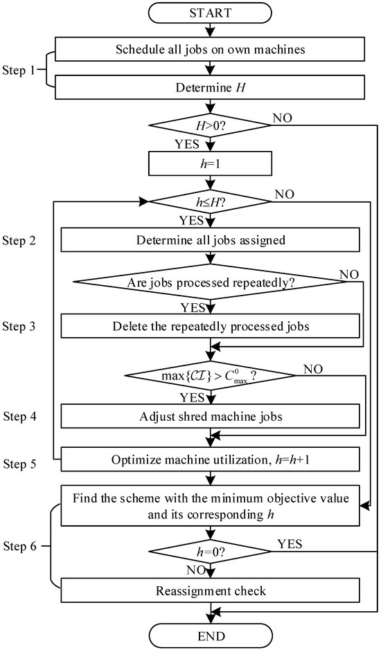
Figure 1.
The heuristic algorithm flowchart.
Step 1. Assign all jobs to owned machines according to the LPT rule to obtain the initial schedule and the target value . According to Property 4, if , then let . If , then set . If , then set . If , then for each h from 1 to H, execute Steps 2 to 5 in sequence. Otherwise, proceed to Step 6.
Step 2. Sort the jobs in non-increasing order based on . Select the jobs sequentially until the sum of the processing times of the selected jobs exceeds , and assign these selected jobs to the owned machines. Then, assign the jobs that satisfy to the owned machines according to Property 3. The jobs of the owned machines are scheduled according to the LPT rule, and the maximum completion time is calculated. The jobs on the shared machines are sorted in non-decreasing order according to , and the completion times of these machines are calculated. Let the set of completion times for the shared machines be . If there are jobs that are processed repeatedly on the shared machines, run Step 3. Otherwise, obtain the feasible schedule and determine whether there is a value greater than in . If so, run Step 4; otherwise, run Step 5.
Step 3. Delete the repeatedly processed jobs, which mainly involves the following two steps:
Step 3.1. Let the set of repeatedly processed jobs on the shared machines be denoted by , and let . If , determine whether there are any repeatedly processed jobs on the machine with a completion time equal to . If so, delete the job with the largest processing position among the repeatedly processed jobs, and update , , and . If not, set the completion time of the corresponding machine in equal to 0, and repeat this step until .
Step 3.2. If , for each repeatedly processed job, retain only the instance on the machine with the smallest ratio of the job processing position to the number of jobs. If multiple machines have equal ratios, retain the job on the machine with the smallest machine number and delete the repeatedly processed jobs on the remaining machines. Sort the jobs on the shared machines by in a non-decreasing order, update , and obtain the schedule . If , run Step 4, otherwise, run Step 5.
Step 4. Let be the shared machine with a completion time equal to . If there are already rented machines with completion times less than (denoted by the set ), proceed to Step 4.1. Then, if , there are unrented machines (denoted by the set ), and , let the number of machines that need to be rented be , and run Step 4.2. Then, if , proceed to Step 4.3. Repeat this step until .
Step 4.1. Adjust the jobs on in sequence. For example, consider the job on . Sort the machines in according to (where ) in non-decreasing order, and determine whether can be moved to each machine for processing in sequence. For instance, consider in . If is moved to , the following conditions must be satisfied: (1) (where if , and otherwise); (2) ; (3) . If all these conditions are met, move to , update and , and do not consider other adjustable machines after . If , there is no need to adjust any other jobs on after .
Step 4.2. If , set ; otherwise, set . Each machine in performs the following operations in sequence. For example, consider machine in : The jobs on are sorted by in non-decreasing order, and the processing times of the jobs that satisfy are added in sequence. When the cumulative sum of the jobs’ processing times is greater than D, stop the summation. Let be the set of jobs whose processing times are summed. If , set ; otherwise, set , where represents the increase in service cost after adjusting the job. After all machines in complete these operations, obtain the sets and . If , identify the machine corresponding to . Move the jobs in from to , and update , , and . Perform the above operation times.
Step 4.3. The jobs on are sorted in non-increasing order based on and are assigned sequentially to the owned machines. When the sum of the processing times of the assigned jobs exceeds , no further jobs from are assigned to the owned machines. Update , schedule the jobs on the owned machines according to the LPT rule, and update and .
Step 5. Let the set of rented machines be , and initialize and . If , identify the machine with the smallest completion time in as , with completion time . If , run Step 6. Otherwise, adjust the jobs on in as follows. For example, consider a job on . Sort the machines in according to in non-decreasing order. Initialize . Determine if can be moved to them for processing in sequence. Take the machine in as an example. If moving to satisfies both and , then move to . Calculate the increase in service cost . Set , update and . No further machines need to be considered after . If , set , . No further jobs need to be judged after . If , set , ; otherwise, set , . Remove from , , and repeat the above operations until . Finally, calculate the target value for .
Step 6. Select the scheduling scheme with the minimum objective value and perform local adjustments to further optimize it.
Step 6.1. Select the scheduling and h corresponding to the minimum objective value from and . If , then is the scheduling result of the algorithm, with the objective value being . Otherwise, let the completion time of all machines be , set , let be the set of rented machines, and let be the set of jobs on the owned machines.
Step 6.2. Find the machine and the job that correspond to . If assigning job to machine and sorting the jobs on the owned machines according to the LPT rule results in a decrease in the objective value, then perform this operation and update and . Otherwise, set . Repeat Step 6.2 until , , or the maximum completion time of the shared machines is greater than or equal to the maximum completion time of the owned machines.
In this heuristic algorithm, the computation times of Step 1 and Step 2 are . The computation time of Step 3 is . The computation times of Step 4.1, Step 4.2, and Step 4.3 are , , and , respectively. Since Step 4.1 to Step 4.3 are executed at most k times, the computation time of Step 4 is . The computation times of Step 5 and Step 6 are and , respectively. Since Step 2 to Step 5 are executed at most k times, the computation time complexity of NSMD-H is .
7. Computation Experiments
This section analyzes the performance of the proposed NSMD-H algorithm through numerical experiments. The mathematical programming model and the algorithm are coded in MATLAB R2024b and executed on a personal computer (Intel Core i7-8550U, 8 GB memory, Windows 11 64 bit). CPLEX12.10 is employed to solve the integer programming model accurately. CPLEX employs its default branch-and-bound algorithm for such problems. The optimal or satisfactory solution is found efficiently by systematically enumerating the space of potential solutions, combined with pruning techniques. The calculation time limit of CPLEX is set to 7200 s. The following will introduce data generation, experimental results, and analysis in sequence.
The problem parameters are randomly generated similar to references [19,22], and the case scale is shown in Table 1.

Table 1.
The related parameter ranges.
For the above cases, CPLEX, NSMD-H, and a Genetic Algorithm (GA) are used to solve the problem, and the LPT rule is used to schedule jobs on the owned machines. The results obtained from these methods are compared and analyzed. The GA algorithm in this section is based on the work in [21], which shares similarities with this paper by considering jobs on both owned and external machines. The GA algorithm from [21] is known for its high computational accuracy. Therefore, the GA algorithm in this section adopts the same individual gene coding representation, mutation operator, and selection operator as in [21]. However, extensive experiments have shown that the single-point crossover operator used in [21] is not well-suited for this problem. Consequently, the GA algorithm in this section employs a two-point crossover operator, specifically for the second half of the parent chromosome. Additionally, the scheduling result obtained from the NSMD-H algorithm is transformed into a chromosome to form part of the initial population for the GA algorithm. An elite retention strategy is also implemented to preserve the individual with the highest fitness after each iteration.
In the GA, four key parameters need to be determined: the iteration number, the population size, the crossover probability, and the mutation probability. Therefore, the Taguchi method of design of experiment (DOE) is used, and the DOE is conducted with the following settings: , , and . For each parameter, three levels are tested. Specifically, for iteration number, [100, 200, 300] for population size, [0.7, 0.8, 0.9] for crossover probability, and [0.1, 0.2, 0.3] for mutation probability are selected. For each combination, the test is repeated 10 times, and the mean value is calculated. The best-combined parameter configuration is as follows: iteration number = 200, population size = 100, crossover probability = 0.7, and mutation probability = 0.3.
A total of 51 sets of experiments are conducted, varying the number of machines, job sizes, and the values of the fixed rental cost a and the unit variable cost b of shared machines. The specific results for small-scale and large-scale cases are presented in Table 2 and Table 3, respectively. A sensitivity analysis is performed on a and b to assess their impact on the experimental results. This analysis examines how changes in a and b (while keeping other parameters constant) affected the outcomes, using the control variable method. The experimental results are shown in Table 4.
Table 2.
Computational results for small-scale problems.
Table 3.
Computational results for large-scale problems.
Table 4.
Computational results for different values of a and b.
Denote the objective value and the number of rented machines obtained by CPLEX as and . The columns Z, , and h record the objective value, calculation time (in seconds), and the number of rented machines of each method, respectively. For the GA, the results shown are the average values obtained from five runs. The relative error gap between the algorithm’s objective value and the optimal value is calculated as . Since the calculation time for scheduling jobs on owned machines using the LPT rule was consistently less than 0.01 s across all cases, the calculation time for LPT is not listed in the tables.
- (1)
- When the number of jobs and machines is small, CPLEX can accurately solve the problem. However, as the scale of the problem increases, its computation time tends to rise significantly, ranging from 0.83s to 7200s. When the number of jobs and machines is large, CPLEX becomes unstable in terms of computational efficiency. In some cases, CPLEX is unable to provide an accurate solution and corresponding scheduling scheme within two hours. For example, this occurs when there are 10 owned machines, 8 shared machines, and 500 jobs or 800 jobs.
- (2)
- The NSMD-H algorithm demonstrates a short computation time, even for large-scale cases with 800 jobs, 10 owned machines, and 10 shared machines, with a running time of only 1.63 s. In terms of computational accuracy, the NSMD-H algorithm performs well. The gap between the objective value obtained using the NSMD-H algorithm and the optimal value obtained using CPLEX ranges from 0.04% to 7.5%. The average gap values for small-scale and large-scale cases are 2.76% and 1.67%, respectively. The difference between the number of rented machines using the NSMD-H algorithm and the number of rented machines based on optimal scheduling is not significant. The maximum difference observed is three machines. This indicates that the objective value is influenced not only by the number of rented machines but also by the scheduling arrangement of jobs.
- (3)
- The computation time of the GA algorithm gradually increases from 2.83 s to 12.78 s, indicating relatively high running efficiency. However, compared to the NSMD-H algorithm, the GA algorithm does not significantly improve solution quality. The average gap values of small-scale and large-scale cases are 2.01% and 1.63%, respectively. Additionally, the number of shared machines rented based on the GA algorithm is consistent with that of the NSMD-H algorithm. The primary reason for this is that the quality of solutions generated by the GA algorithm through random chromosome initialization differs significantly from that of the NSMD-H algorithm. Consequently, the better solutions obtained during GA iterations are mostly local adjustments to the solutions initially obtained using the NSMD-H algorithm. This results in minimal changes to the objective value. Therefore, the GA algorithm, while increasing computation time, does not significantly enhance the quality of solutions obtained by the NSMD-H algorithm.
- (4)
- The LPT rule, which schedules jobs only on owned machines without considering rented machines, has a very low computation time (no more than 0.01 s). However, it deviates significantly from optimal scheduling. In some cases, the maximum deviation reaches 95.25%.
The following conclusions can be drawn from analyzing Table 4:
- (1)
- When other parameters remain unchanged, an increase in the fixed rental cost a leads to a higher objective value and a gradual decrease in the number of shared machines rented. The same trend is observed for the unit variable rental cost b.
- (2)
- The conclusions drawn from analyzing Table 2 and Table 3 are consistent. CPLEX exhibits significant variability in computational efficiency, with computation times ranging from 1.47 s to 99.54 s. The values of parameters a and b have a substantial impact on CPLEX’s computational time, with no discernible pattern.
- (3)
- The NSMD-H and GA algorithms demonstrate high computational efficiency, unaffected by the values of a and b. The average computational times are 0.21 s and 4.38 s, respectively. Both algorithms achieve higher computational accuracy, with average deviations of 3.15% and 2.82%, respectively.
- (4)
- All jobs are scheduled on owned machines using the LPT rule. The objective value is independent of the values of a and b. However, the deviation from the optimal value is significant, particularly in cases where the shared machine rental cost is low and the optimal number of rented machines is high (e.g., the 1st and 10th cases in the table). As previously noted, when parameters n, a, b, and take extreme values, the deviation becomes unbounded.
In summary, the NSMD-H and GA algorithms are effective in solving the problem, maintaining high computational accuracy and solution efficiency even as the problem size increases. While both algorithms achieved similar levels of computational accuracy, the NSMD-H algorithm demonstrated superior computational efficiency, meeting the dual requirements of solution quality and computational speed necessary for practical production environments.
The primary motivation for studying this machine-sharing scheduling problem is to provide a theoretical foundation for enterprise managers to make informed decisions regarding the rental of shared machines and the arrangement of job production schedules. Through mathematical modeling, property analysis, algorithm design, and problem-solving, the following management insights are offered to assist enterprise decision-makers:
- (1)
- The rental and scheduling results of machines are influenced by multiple factors. Enterprises should comprehensively consider their own production conditions (such as the number of owned machines), the characteristics of jobs to be processed (including the number of jobs and their processing times), the production goals of the enterprise, and the costs associated with shared machines (fixed rental costs, unit variable costs, shared service costs).
- (2)
- Enterprises can utilize the proposed model and algorithm to determine the number of shared machines to be rented and to arrange the order of jobs on their own machines and shared machines. This approach helps reduce the maximum completion time of jobs (i.e., customer waiting time) while optimizing the enterprise’s shared costs. For small-scale problems, the model can be used to obtain exact solutions. For large-scale problems, the proposed algorithm can efficiently generate near-optimal solutions to support decision-making.
8. Conclusions
This paper examined an offline scheduling problem for identical parallel machines, incorporating the practical scenario of renting shared machines in manufacturing enterprises. Manufacturers with a certain number of machines can rent additional shared machines to process jobs. However, they must incur fixed rental costs, unit variable rental costs, and shared service costs associated with both jobs and machines. The optimization objective is to minimize the sum of the makespan and the total shared cost. To address this problem, an integer linear programming model was first developed and solved by the commercial solver, CPLEX. Subsequently, the optimal scheduling without renting machines and the range of optimal rental quantities when renting machines were analyzed. Based on the problem’s properties, the NSMD-H algorithm for large-scale problems was designed and applied to solve the considered problem. Furthermore, experiments were carried out to compare the proposed NSMD-H algorithm with GA and LPT rule. Compared with the GA algorithm, the designed algorithm had a higher solving efficiency and smaller gap values. Compared with the LPT rule, the designed algorithm had a higher calculational accuracy. Sensitivity analyses further showed that the number of shared machines decreased with the both the fixed rental cost and the unit variable rental cost, while the corresponding objective value increased.
In summary, shared machine scheduling becomes more necessary in optimizing the allocation of resources, improving productivity, and promoting sustainable industrial synergies. All of this leads to greater sustainability in manufacturing. Manufacturers can strategically implement the NSMD-H algorithm according to their specific production parameters, shared resource availability, and associated cost structures. This approach can effectively reduce both job completion times and machine-shared costs. By optimizing resource utilization efficiency and minimizing idle resource waste, the algorithm facilitates long-term equilibrium in socioeconomic systems while advancing sustainable development goals.
Future research directions may include (i) designing heuristics that can solve the problem more efficiently; (ii) considering more practical conditions, such as various rental discounts and multi-resource sharing; (iii) investigating scheduling problems where jobs are processed on shared machines of different machine types (e.g., uniform parallel machines, unrelated parallel machines, etc.); and (iv) studying the problem with other objective functions, such as scheduling problems with durations (maximum delay time, delay time, number of late jobs, etc.) or multi-objective functions.
Author Contributions
Conceptualization, Y.X. and R.Z.; methodology, R.Z. and F.Z.; software, R.Z.; validation, R.Z.; writing—original draft preparation, R.Z. and F.X.; writing—review and editing, R.Z. and F.Z. All authors have read and agreed to the published version of the manuscript.
Funding
This work was supported by the National Natural Science Foundation of China (NSFC) under Grants 72271051, 72071144 and 71832001. This work was also supported by the Fundamental Research Funds for the Central Universities under Grant 2232018H-07.
Institutional Review Board Statement
Not applicable.
Informed Consent Statement
Not applicable.
Data Availability Statement
The raw data supporting the conclusions of this article will be made available by the authors on request.
Acknowledgments
The authors would like to thank the anonymous referees for their constructive comments.
Conflicts of Interest
The authors declare no conflicts of interest.
Appendix A
Proof of Property 2.
Let denote the optimal maximum completion time of n jobs allocated to m owned machines. If a shared machine is added, let represent the optimal maximum completion time of n jobs allocated to machines, and let be the minimum machine completion time. Then, . Since jobs are non-interruptible, . Therefore, adding a machine can reduce by at most (i.e., ). When the fixed rental cost a of the newly added shared machine is greater than or equal to the maximum reduction in the maximum completion time, the optimal scheduling does not rent a shared machine. □
Proof of Property 4.
When the shared service cost is not considered, let denote the optimal value of the interruptible scheduling problem, with representing the number of shared machines rented in the optimal scheduling scenario. Similarly, let denote the optimal value of the non-interruptible scheduling problem, with representing the number of machines rented in the optimal scheduling. We first prove that . Next, we demonstrate that in the optimal scheduling of the interruptible problem, for , the machine completion time is equal to . Finally, we determine the value of in the interruptible problem.
① It is evident that . This inequality holds because the reduction in the maximum completion time when jobs can be interrupted is greater than or equal to the increase in rental costs. One possible reason for the increase in rental costs is the higher number of rented machines, implying that . Moreover, since the problem accounts for the shared service cost , which can potentially reduce the number of rented machines, it follows that .
② In the interruptible scheduling problem without considering the shared service cost. (i) Since renting a shared machine incurs a unit variable cost (), the maximum completion time of the owned machines is greater than or equal to that of the rented machines; (ii) If the completion times of the owned machines are not equal, adjusting them to be equal can reduce ; (iii) If the completion times of the rented machines are not equal, adjusting them to be equal will not change the target value; (iv) If the completion times of the owned machines are greater than those of the rented machines, adjust them to be equal. If the target value increases, then , and the completion times of the owned machines are equal to . Otherwise, , and the completion times of the used machines are equal to . For any scheduling , if the above four situations exist, the optimal scheduling can be obtained through appropriate adjustments. Figure A1 illustrates the effects of these adjustments schematically. Since the scheduling of jobs on each machine is not shown, the symbol “” is used in the diagram to simplify the representation.
③ In the interruptible scheduling problem, without considering the shared service cost, for , the machine completion time is equal to . This leads to . Define the function . The first and second derivatives of are and , respectively. When , the second derivative is positive, and the first derivative increases monotonically. Currently, minimizes at when , at when , and at when . When , the first derivative is positive, indicating that is monotonically increasing. The minimum value of occurs at . □

Figure A1.
The scheduling effect diagram of arbitrary scheduling adjustment to optimal scheduling.
Figure A1.
The scheduling effect diagram of arbitrary scheduling adjustment to optimal scheduling.

References
- Wang, G.; Zhang, G.; Guo, X.; Zhang, Y.F. Digital twin-driven service model and optimal allocation of manufacturing resources in shared manufacturing. J. Manuf. Syst. 2021, 59, 165–179. [Google Scholar] [CrossRef]
- Liu, C.Y.; Liu, P. Dynamic allocation of manufacturing tasks and resources in shared manufacturing. Intell. Autom. Soft. Comput. 2023, 36, 3221–3242. [Google Scholar] [CrossRef]
- Liu, P.; Wei, X.L. Three-party evolutionary game of shared manufacturing under the leadership of core manufacturing company. Sustainability 2022, 14, 13682. [Google Scholar] [CrossRef]
- Patterson, S.R.; Kozan, E.; Hyland, P. Energy efficient scheduling of open-pit coal mine trucks. Eur. J. Oper. Res. 2017, 262, 759–770. [Google Scholar] [CrossRef]
- Vélez-Gallego, M.C.; Maya, J.; Montoya-Torres, J.R. A beam search heuristic for scheduling a single machine with release dates and sequence dependent setup times to minimize the makespan. Comput. Oper. Res. 2016, 73, 132–140. [Google Scholar] [CrossRef]
- Zhao, D.Z.; Wang, Z.S. Scheduling optimization of cloud manufacturing platform processing capability sharing. Oper. Res. Manag. Sci. 2016, 28, 1–6. (In Chinese) [Google Scholar]
- Yu, Y.N.; Xu, Z.; Liu, D.N. Distributed multi-project scheduling problem with multi-skilled staff. Syst. Eng. Theor. Pract. 2020, 40, 2921–2933. (In Chinese) [Google Scholar]
- Tang, L.; Han, H.Y.; Tan, Z.; Jing, K. Centralized collaborative production scheduling with evaluation of a practical order-merging strategy. Int. J. Prod. Res. 2023, 61, 282–301. [Google Scholar] [CrossRef]
- Kuroda, M. Integration of product design and manufacturing through real-time due-date estimation and scheduling systems. J. Adv. Mech. Des. Syst. 2016, 10, JAMDSM42. [Google Scholar] [CrossRef][Green Version]
- Edis, E.B.; Oguz, C. Parallel machine scheduling with flexible resources. Comput. Ind. Eng. 2012, 63, 433–447. [Google Scholar] [CrossRef]
- Fanjul-Peyro, L.; Perea, F.; Ruiz, R. Models and matheuristics for the unrelated parallel machine scheduling problem with additional resources. Eur. J. Oper. Res. 2017, 260, 482–493. [Google Scholar] [CrossRef]
- Ostojic, D.; Ramljak, D.; Urosevic, A.; Jolovic, M.; Draskovic, R.; Kakka, J.; Krüger, T.J.; Davidovic, T. Systematic literature review of optimization algorithms for P||Cmax problem. Symmetry 2025, 17, 178. [Google Scholar] [CrossRef]
- Ji, B.; Zhang, S.J.; Yu, S.S.; Xiao, X.; Chen, C.; Zheng, G.H. Novel model and solution method for flexible job shop scheduling problem with batch processing machines. Comput. Oper. Res. 2024, 161, 106442. [Google Scholar] [CrossRef]
- Hao, L.Y.; Zou, Z.Y.; Liang, X. Solving multi-objective energy-saving flexible job shop scheduling problem by hybrid search genetic algorithm. Comput. Ind. Eng. 2025, 200, 110829. [Google Scholar] [CrossRef]
- Becker, T.; Neufeld, J.; Buscher, U. The distributed flow shop scheduling problem with inter-factory transportation. Eur. J. Oper. Res. 2025, 322, 39–55. [Google Scholar] [CrossRef]
- Wang, Y.; Jin, H.J.; Wang, G.G.; Wang, L. A bi-population cooperative discrete differential evolution for multiobjective energy-efficient distributed blocking flow shop scheduling problem. IEEE Trans. Syst. Man Cybern. Syst. 2025, 55, 2211–2223. [Google Scholar] [CrossRef]
- Dereniowski, D.; Kubiak, W. Shared multi-processor scheduling. Eur. J. Oper. Res. 2017, 261, 503–514. [Google Scholar] [CrossRef]
- Dereniowski, D.; Kubiak, W. Shared processor scheduling of multiprocessor jobs. Eur. J. Oper. Res. 2020, 282, 464–477. [Google Scholar] [CrossRef]
- Li, K.; Zhang, H.J.; Cheng, B.Y.; Pardalos, P.M. Uniform parallel machine scheduling problems with fixed machine cost. Optim. Lett. 2018, 12, 73–86. [Google Scholar] [CrossRef]
- Ji, M.; Ye, X.N.; Qian, F.Y.; Cheng, T.C.E.; Jiang, Y.W. Parallel-machine scheduling in shared manufacturing. J. Ind. Manag. Optim. 2022, 18, 681–691. [Google Scholar] [CrossRef]
- Xu, Y.F.; Zhi, R.T.; Zheng, F.F.; Liu, M. Parallel machine scheduling with due date-to-deadline window, order sharing and time value of money. Asia Pac. J. Oper. Res. 2022, 39, 2150024. [Google Scholar] [CrossRef]
- Zheng, F.F.; Jin, K.Y.; Xu, Y.F.; Liu, M. Parallel machine scheduling with order splitting and matching type. Oper. Res. Manag. Sci. 2023, 32, 1–7. (In Chinese) [Google Scholar]
- Xu, Y.F.; Zhi, R.T.; Zheng, F.F.; Liu, M. Competitive algorithm for scheduling of sharing machines with rental discount. J. Comb. Optim. 2022, 44, 414–434. [Google Scholar] [CrossRef]
- Xu, Y.F.; Zhi, R.T.; Zheng, F.F.; Liu, M. Online strategy and competitive analysis of production order scheduling problem with rental cost of shared machines. Chin. J. Manag. Sci. 2023, 31, 142–150. (In Chinese) [Google Scholar]
- Cheng, J.H.; Cheng, J.Y.; Lin, Y.H.; Lu, S.; Wu, P. MILP models and effective heuristic for energy-aware parallel machine scheduling with shared manufacturing. Expert Syst. Appl. 2025, 271, 126681. [Google Scholar] [CrossRef]
- Wei, Q.; Wu, Y. Two-machine hybrid flow-shop problems in shared manufacturing. CMES—Comput. Model. Eng. Sci. 2022, 131, 1125–1146. [Google Scholar] [CrossRef]
- Fu, Y.P.; Li, H.B.; Huang, M.; Xiao, H. Bi-objective modeling and optimization for stochastic two-stage open shop scheduling problems in the sharing economy. IEEE Trans. Eng. Manag. 2023, 70, 3395–3409. [Google Scholar] [CrossRef]
- Akaria, I.; Epstein, L. An optimal online algorithm for scheduling with general machine cost functions. J. Sched. 2020, 23, 155–162. [Google Scholar] [CrossRef]
- Dai, B.F.; Li, W.D. Vector scheduling with rejection on two machines. Int. J. Comput. Math. 2020, 97, 2507–2515. [Google Scholar] [CrossRef]
- Shabtay, D.; Gerstl, E. Coordinating scheduling and rejection decisions in a two-machine flow shop scheduling problem. Eur. J. Oper. Res. 2024, 316, 887–898. [Google Scholar] [CrossRef]
- Choi, B.C.; Park, M.J. Single-machine scheduling with resource-dependent processing times and multiple unavailability periods. J. Sched. 2022, 25, 191–202. [Google Scholar] [CrossRef]
- Choi, B.C.; Lee, J.H. A resource allocation problem with convex resource-dependent processing times under a two-machine flow shop environment. Asia Pac. J. Oper. Res. 2024, 41, 2350018. [Google Scholar] [CrossRef]
- Choi, B.C.; Chung, J. Two-machine flow shop scheduling problem with an outsourcing option. Eur. J. Oper. Res. 2011, 213, 66–72. [Google Scholar] [CrossRef]
- Lu, L.F.; Zhang, L.Q.; Ou, J.W. In-house production and outsourcing under different discount schemes on the total outsourcing cost. Ann. Oper. Res. 2021, 298, 361–374. [Google Scholar] [CrossRef]
- Ma, R.; Yuan, J.J. Online scheduling to minimize the total weighted completion time plus the rejection cost. J. Comb. Optim. 2017, 34, 483–503. [Google Scholar] [CrossRef]
- Mokhtari, H.; Abadi, I.N.K. Scheduling with an outsourcing option on both manufacturer and subcontractors. Comput. Oper. Res. 2011, 213, 66–72. [Google Scholar] [CrossRef]
- Yin, Y.; Cheng, T.C.E.; Wang, D.; Wu, C.C. Improved algorithms for single-machine serial-batch scheduling with rejection to minimize total completion time and total rejection cost. IEEE Trans. Syst. Man Cybern. Syst. 2016, 46, 1578–1588. [Google Scholar] [CrossRef]
- Wang, S.J.; Cui, W.L. Approximation algorithms for the min-max regret identical parallel machine scheduling problem with outsourcing and uncertain processing time. Int. J. Prod. Res. 2021, 59, 4579–4592. [Google Scholar] [CrossRef]
- Ruiz-Torres, A.J.; López, F.J.; Wojciechowski, P.J.; Ho, J.C. Parallel machine scheduling problems considering regular measures of performance and machine cost. J. Oper. Res. Soc. 2010, 61, 849–857. [Google Scholar] [CrossRef]
- Rustogi, K.; Strusevich, V.A. Parallel machine scheduling: Impact of adding extra machines. Oper. Res. 2013, 61, 243–257. [Google Scholar] [CrossRef]
- Lee, K.; Leung, J.Y.-T.; Jia, Z.H.; Li, W.H.; Pinedo, M.L.; Lin, B.M.T. Fast approximation algorithms for bi-criteria scheduling with machine assignment costs. Eur. J. Oper. Res. 2014, 238, 54–64. [Google Scholar] [CrossRef]
- Li, K.; Zhang, X.; Leung, J.Y.-T.; Yang, S.L. Parallel machine scheduling problems in green manufacturing industry. J. Manuf. Syst. 2016, 38, 98–106. [Google Scholar] [CrossRef]
- Li, K.; Xu, S.L.; Cheng, B.Y.; Yang, S.L. Parallel machine scheduling problem with machine cost to minimize the maximal lateness. Syst. Eng. Theor. Pract. 2019, 39, 165–173. (In Chinese) [Google Scholar]
- Jiang, Y.W.; Tang, X.L.; Li, K.; Cheng, T.C.E.; Ji, M. Approximation algorithms for bi-objective parallel-machine scheduling in green manufacturing. Comput. Ind. Eng. 2023, 176, 108949. [Google Scholar] [CrossRef]
- Anghinolfi, D.; Paolucci, M.; Ronco, R. A bi-objective heuristic approach for green identical parallel machine scheduling. Eur. J. Oper. Res. 2021, 289, 416–434. [Google Scholar] [CrossRef]
- Jarboui, B.; Masmoudi, M.; Eddaly, M. Epsilon Oscillation Algorithm for the bi-objective green identical parallel machine scheduling problem. Comput. Oper. Res. 2024, 170, 106754. [Google Scholar] [CrossRef]
- Wu, P.; Wang, Y.; Chu, C. Logic-based Benders decomposition for bi-objective parallel machine selection and job scheduling with release dates and resource consumption. Comput. Oper. Res. 2024, 164, 106528. [Google Scholar] [CrossRef]
- Lenstra, J.K.; Rinnooy Kan, A.H.G.; Brucker, P. Complexity of machine scheduling problems. Ann. Discrete Math. 1977, 1, 343–362. [Google Scholar]
- McNaughton, R. Scheduling with deadlines and loss functions. Manag. Sci. 1959, 6, 1–12. [Google Scholar] [CrossRef]
- Graham, R.L. Bounds on multiprocessing time anomalies. SIAM J. Appl. Math. 1969, 17, 416–429. [Google Scholar] [CrossRef]

Disclaimer/Publisher’s Note: The statements, opinions and data contained in all publications are solely those of the individual author(s) and contributor(s) and not of MDPI and/or the editor(s). MDPI and/or the editor(s) disclaim responsibility for any injury to people or property resulting from any ideas, methods, instructions or products referred to in the content. |
© 2025 by the authors. Licensee MDPI, Basel, Switzerland. This article is an open access article distributed under the terms and conditions of the Creative Commons Attribution (CC BY) license (https://creativecommons.org/licenses/by/4.0/).