Abstract
Slope stability analysis requires particular attention to groundwater effects, where seepage–stress coupling fundamentally alters mechanical responses. This investigation develops a field-calibrated numerical model using monitoring data from a water diversion project in Yunnan, using finite element analysis based on seepage–stress coupling theory. Comparative stability assessments through strength reduction methodology evaluate three scenarios: non-seepage conditions, seepage–stress interaction, and cutoff wall implementation. Results demonstrate the cutoff wall’s effectiveness, achieving optimal slope ratios of 1:1.41 compared to 1:2.21 under seepage–stress coupling. Parametric analyses reveal quantitative relationships between wall characteristics and stability metrics. Elastic modulus optimization within practical ranges (9362.63 MPa peak performance) enables steeper 1:1.37 slopes while maintaining safety factors. Strategic width reduction from 0.6 m to 0.4 m decreases concrete usage by 33% without compromising stability thresholds, proving cost-efficiency in large-scale applications. The methodology provides actionable guidelines for deep excavation projects facing similar hydrogeological challenges. Optimized cutoff walls enhance slope stability sustainably through ecological preservation and resource efficiency, providing actionable frameworks for eco-conscious geotechnical design aligned with global sustainability objectives.
1. Introduction
Seepage control in slope engineering remains a critical challenge in geotechnical practice [1,2,3]. The rapid expansion of global infrastructure has increased demand for high-steep slopes, where hydromechanical coupling effects induced by seepage have been identified as primary instability triggers [4,5,6,7]. Traditional anti-seepage systems like drainage trenches and relief wells, while effective in reducing pore pressure, face limitations in complex geological settings due to high maintenance costs and long-term performance degradation [8,9,10,11]. Cutoff walls have consequently emerged as a core solution for high-risk slopes, functioning through dual mechanisms: physically obstructing seepage paths to modify hydraulic gradients while participating in stress redistribution as structural elements [12,13,14]. This mechano–hydraulic coupling endows cutoff walls with safety-economic synergy, though the dynamic relationship between wall stiffness and slope stability remains insufficiently characterized, hindering refined engineering applications.
Research on cutoff wall mechanisms has progressed through distinct phases. Early studies employing limit equilibrium methods established analytical formulas for seepage quantification, demonstrating the necessity for wall permeability coefficients significantly lower than surrounding soils [15,16,17,18,19]. However, prediction errors reached 25% in complex seepage fields due to unaccounted stress redistribution [20,21]. Advancements in numerical simulations enabled adoption of strength reduction methods, revealing that stiffness increases alter principal stress orientations in backfill soils, causing potential slip surfaces to migrate deeper—a finding transcending traditional hydraulic design paradigms [22,23,24,25]. Computational constraints initially restricted models to idealized elastoplastic assumptions, inadequately capturing material nonlinearity [26,27].
Emerging international studies have advanced understanding of cutoff wall mechanics through enhanced computational frameworks [28,29]. Recent advances in numerical modeling have employed discrete element-fluid coupling approaches to reveal how stress-dependent permeability evolution governs interfacial hydraulic fracturing mechanisms [30]. Multiphysics simulations incorporating unsaturated flow–stress interactions have further identified critical stiffness thresholds that mitigate differential settlement in stratified geological formations [31]. Machine learning applications are demonstrating potential for optimizing wall configurations by synthesizing multiple geological parameters, achieving cost-effective solutions while preserving stability margins [32]. These computational advancements have complemented material innovations by addressing nonlinear interactions between hydraulic processes and mechanical responses, while introducing novel paradigms for performance prediction under complex hydrogeological conditions.
Recent breakthroughs in wall materials have exposed critical trade-offs: cement–bentonite composites exhibit permeability degradation with stiffness enhancement, while fiber-reinforced materials improve ductility without compromising impermeability [33]. Parametric optimization using strength reduction methods coupled with response surface methodology revealed nonlinear relationships between optimal wall stiffness and soil permeability anisotropy, though excavation effects remain unaddressed [34,35,36]. Current design codes rely on empirical safety factor approaches, relying on engineering analogies for stiffness selection that often yield over-conservative or under-designed solutions [37,38].
Persistent scientific challenges include stiffness-induced deformation incompatibility triggering interfacial hydraulic fracturing; unestablished constitutive models for bidirectional seepage–stress coupling affecting slip surface development; and multi-objective optimization under economic constraints to transcend conventional slope ratio thresholds [39,40,41,42,43].
This study establishes coupled seepage–stress numerical models combined with parametric testing to systematically investigate stiffness effects. Strength reduction methods accurately characterize stress redistribution and progressive failure, identifying an optimal stiffness range maximizing safety factors. The mechanism involves insufficient stress redistribution at low stiffness versus interfacial stress concentration at excessive stiffness. The innovation lies in quantifying nonlinear stiffness–slope ratio coupling and proposing an optimization methodology converting safety redundancy into economic benefits.
2. Field Work
2.1. The Study Site
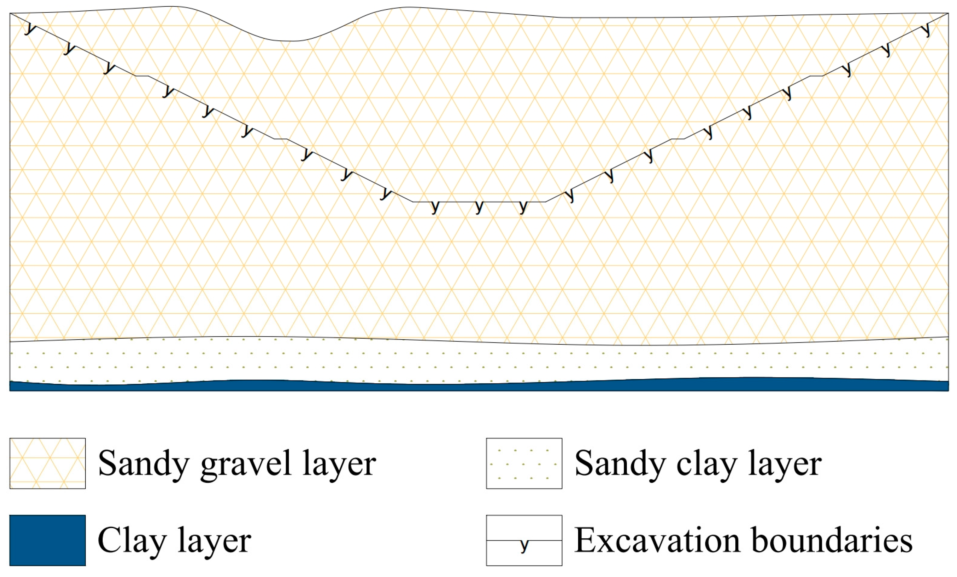
This study focuses on the deep excavation slope of an intake box culvert within a water diversion project located in western Yunnan Province. The engineering site encompasses the Chongjiang River estuary and adjacent right-bank mountainous terrain. The Chongjiang River flows northeast with a bed elevation ranging from 1820 m to 1830 m, while surrounding mountain peaks reach elevations between 2500 m and 2900 m, exhibiting slope angles of 35–40°. Groundwater depth in the riverbed section varies from 2.2 m to 4.15 m, underlain by alluvial–proluvial deposits dominated by sandy gravel cobbles interspersed with boulders (Figure 1). Borehole data indicate that these deposits attain a maximum thickness of 132.8 m, containing localized lenticular silty clay layers. Surface materials consist of 2–3 m thick clay and sandy clay strata. The region experiences an annual precipitation of 753.7 mm, with 91.3% concentrated between May and October, alongside an annual evaporation of 1166 mm. Temperature records show a mean of 12.0 °C with extremes from −11.0 °C to 32.0 °C, while wind speeds average 2.5 m/s, reaching maximums of 20.3 m/s.
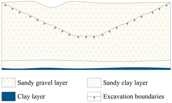
Figure 1.
Excavation boundaries and lithological characteristics in the project area.
Situated within the tectonically active Three Rivers Orogen in the Hengduan Mountains, the project area’s significant topographic relief necessitated deep excavation methods to ensure structural integrity of the box culvert. The predominant sandy cobble gravel lithology demonstrates high permeability and poor self-stabilization characteristics, rendering tunnel construction methods unsuitable due to risks of water infiltration and collapse, as well as excessive equipment wear. The rectangular box culvert configuration requires substantial working space for formwork installation and concrete placement, operational requirements optimally addressed through open excavation techniques that enhance construction efficiency while maintaining quality control standards.
2.2. Slope Surface Deformation Monitoring
In this study, to monitor surface deformation, a total station (Figure 2d) was employed for systematic monitoring of the slope surface. The elevation at the crest of the slope is 1831.1 m. Monitoring points were established at distances of 2 m, 4 m, 6 m, 8 m, 10 m, 14 m, 18 m, 24 m, and 30 m from the slope crest (extending to the toe of the slope) (Figure 2a). Monitoring stakes were installed at each of these points, and a total station was used for regular monitoring.
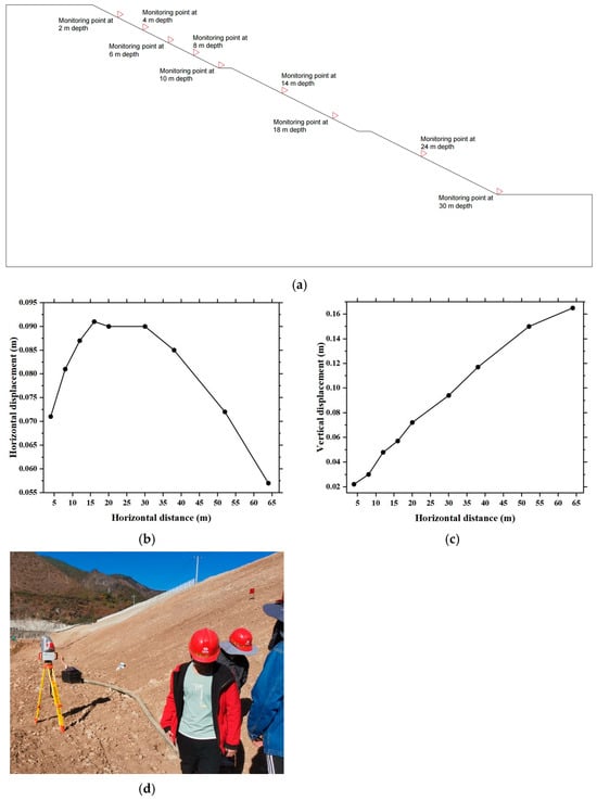
Figure 2.
Slope surface deformation monitoring. (a) Monitoring point locations; (b) horizontal displacement data; (c) vertical displacement data; (d) instrument installation.
Following one month of slope surface deformation monitoring, maximum displacements of 0.091 m (Figure 2b) in the horizontal direction and 0.165 m (Figure 2c) in the vertical direction were recorded. The monitoring data demonstrate distinct deformation characteristics between horizontal and vertical dimensions, with vertical displacements exhibiting 81.3% greater magnitude than horizontal movements. Vertical displacements predominantly concentrate at the slope toe region due to unloading rebound mechanisms, demonstrating characteristic deformation patterns associated with excavation-induced stress redistribution.
2.3. Cutoff Wall Deformation Monitoring
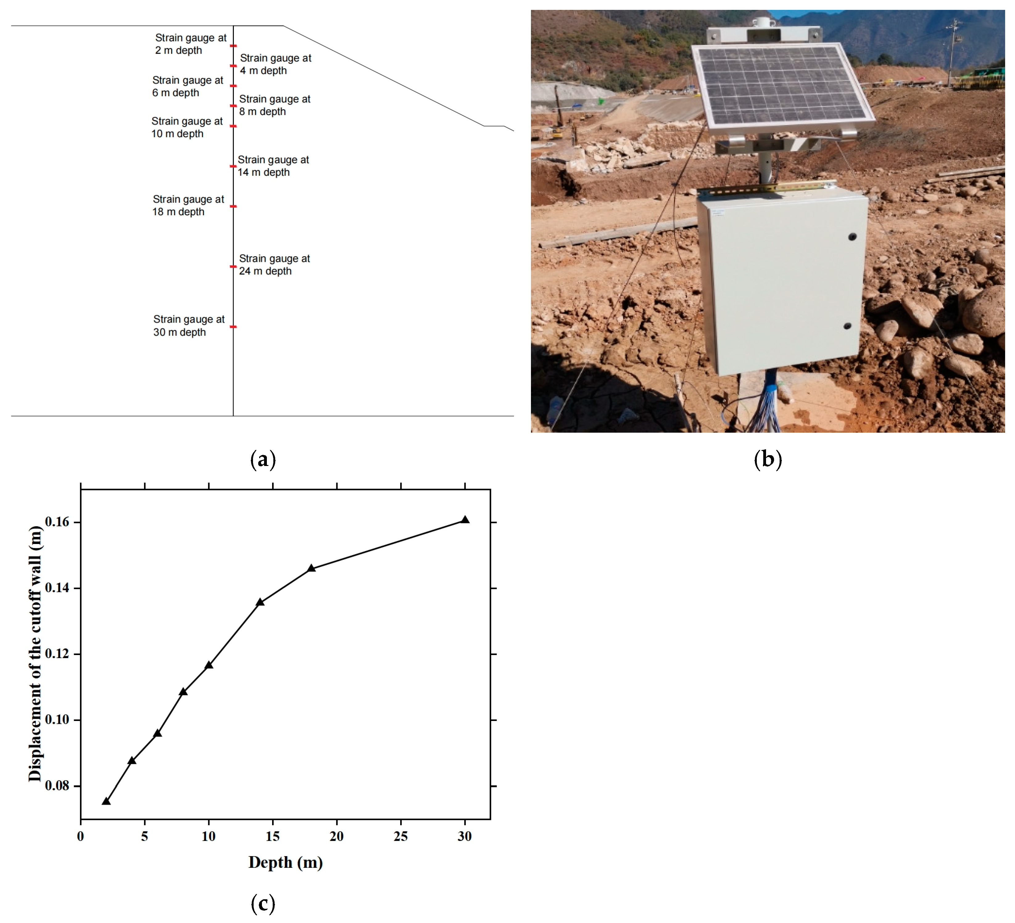
The specific deformation monitoring plan for the cutoff wall was outlined as follows: Before the concrete was poured, strain gauges were embedded at depths of 2 m, 4 m, 6 m, 8 m, 10 m, 14 m, 18 m, 24 m, and 30 m within the cutoff wall (Figure 3a), with each specified depth having one strain gauge. Additionally, no-stress meters were installed at depths of 8 m and 18 m, with one at each site. The instruments were secured by binding them to the reinforcement bars. Initial readings were documented, along with the data collected after the slope excavation was completed.
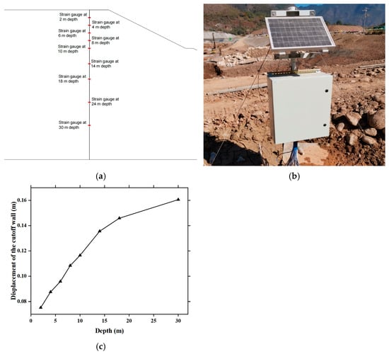
Figure 3.
Cutoff wall deformation monitoring. (a) Strain gauge locations on the cutoff wall; (b) instrument installation; (c) horizontal displacement data.
Based on the monitoring data, the displacement of the cutoff wall increased monotonically from shallow to deep, reaching a maximum value at a depth of 30 m, with the maximum displacement being 0.1606 m (Figure 3c).
3. Mechanism of Seepage–Stress Coupling Interaction
In the context of geotechnical engineering, geomaterials are often complex porous media primarily influenced by seepage fields and stress fields. These two fields interact and mutually affect each other. When a hydraulic head difference developed within the geomaterial, water within the pores induced seepage flow, generating hydrodynamic pressure that acted on the geomaterial. Over time, this hydrodynamic pressure applied as an external load altered the original stress state of the geomaterial. Changes in the stress field caused displacements in the soil particle field, leading to variations in the spacing between soil particles and consequently altering the porosity and void ratio of the geomaterial. Since porosity and void ratio are key parameters determining the permeability coefficient, changes in permeability also resulted in variations in seepage velocity, ultimately affecting the entire seepage field. Therefore, the stress field and the seepage field interacted and influenced each other.
Due to the presence of numerous pores within the geotechnical body, groundwater seepage occurred along these pores under the influence of hydraulic head differences. The seepage body forces acted on the geotechnical body, altering the spatial arrangement of the particles and consequently changing the original stress field of the geotechnical material.
According to the principles of hydraulics, in a continuous medium, the seepage-induced body force was proportional to the hydraulic gradient. It was expressed by the following equation:
where = seepage body force; = hydraulic gradient; = the component of the seepage body force in the x-direction; = the component of the seepage body force in the -direction; = the component of the seepage body force in the z-direction; = the angle between and ; = the angle between and ; = the angle between and ; = the component of the hydraulic gradient in the x-direction; = the component of the hydraulic gradient in the y-direction; = the component of the hydraulic gradient in the z-direction.
When solving the stress field using the finite element method, the seepage body force of an element was transformed into equivalent nodal loads. The specific expression was given by:
where = the element shape function; = the equivalent nodal forces of seepage body forces.
The geotechnical body, classified as a porous medium rather than a fully dense material, underwent changes in its internal spatial structure when subjected to external loads. While the soil particles themselves were incompressible, the distances between particles varied, which altered the porosity and void ratio within the soil body. This, in turn, indirectly led to changes in the permeability coefficient, affecting the intensity of seepage flow. This phenomenon explained the reasons behind the changes in the seepage field induced by variations in the stress field.
The fluid permeability coefficient was expressed as:
where = permeability coefficient (cm/s); = coefficient of permeability (cm2); = The viscosity of the fluid (Pa·s); = the kinematic viscosity coefficient (cm2/s).
From Equation (5), it was determined that the primary factors affecting the permeability of geotechnical materials were the properties of the geotechnical framework itself and the properties of the fluid. The properties of the geotechnical framework were mainly associated with the intrinsic permeability (), while the characteristics of the fluid were predominantly related to its density () and viscosity coefficient (). Among these, porosity was identified as the most significant factor influencing permeability, with permeability generally increasing as porosity increased.
The mathematical model describing the influence of the seepage field on the stress field was presented as:
where = the normal direction of boundary ; = the normal direction of boundary .
The mathematical model depicting the influence of the stress field on the seepage field was described as follows:
where = the differential operator matrix; = the hydraulic head distribution function within the seepage field and formulated as a constant-term column vector for nodes with known head values; = the external load matrix of the nodes; = the displacement field; = specified boundary with known surface tractions; = direction cosine matrix in the normal direction of surface traction boundary; = displacement boundary; = surface force distribution of ; = displacement vector on .
By combining the Equations (6) and (7), which describe the interaction between the seepage field and the stress field, we obtain the coupled model:
where = permeability coefficient correlation matrix; = seepage force matrix related to the hydraulic gradient; = global stiffness matrix.
4. Numerical Simulation Experiment
4.1. Establish the Numerical Model
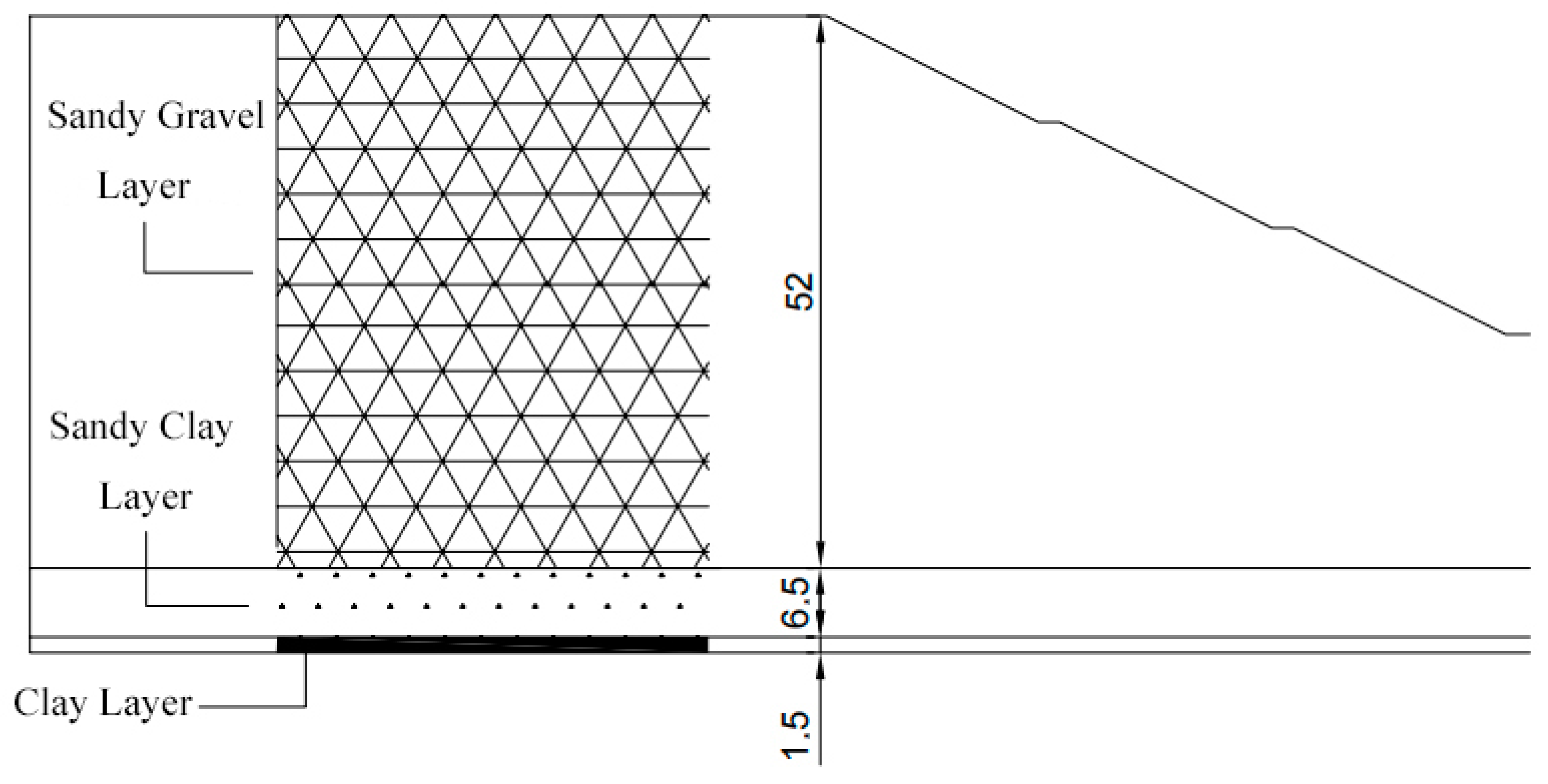
Borehole data (Figure 4) reveal the stratigraphic composition of the Phase II intake culvert slope in this study, consisting sequentially from surface to depth of a sandy gravel layer, sandy clay layer, and clay layer. The actual engineering project (Figure 5) configured the total excavation depth at 30 m, implemented through a benching excavation strategy with 6 m vertical intervals per excavation stage. Safety berms measuring 2 m in width were constructed at 10 m vertical intervals along the excavation face. The slope was cut at a 1:2 gradient, corresponding to a slope angle of 26.57°, with the crest extending 75 m and the toe spanning 45 m in length.
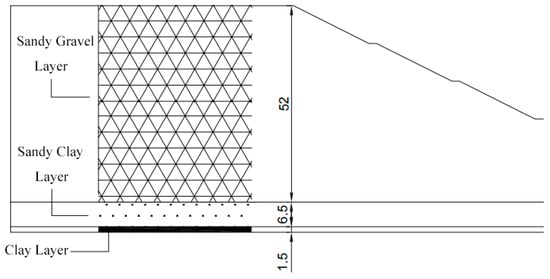
Figure 4.
Stratigraphic distribution of the slope.
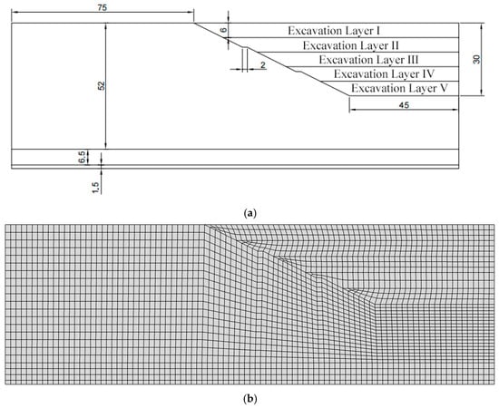
Figure 5.
Model geometry information. (a) Slope dimensional parameters; (b) model meshing.
The core samples of sandy gravel, sandy clay, and clay strata obtained from drilling were processed into standard specimens, while standard specimens of plastic concrete with the same mix proportion as that used in the impervious cutoff wall of the actual engineering project were prepared. Laboratory geotechnical tests were subsequently conducted using these specimens to determine the physical properties of each stratum and the impervious cutoff wall in the study area (Table 1).

Table 1.
Key physical and mechanical parameters of each stratum.
The numerical model was constructed using the ABAQUS/Standard finite element software, which enables coupled seepage–stress analysis through Biot’s consolidation theory and the van Genuchten mode.
The model was directly established based on the theoretical framework of seepage–stress coupling proposed in Chapter 3 (Equations (6)–(8)). Specifically, the seepage-induced volumetric forces (Equation (6)) were converted into equivalent nodal loads via finite element integration, and coupled solutions were achieved through Biot’s consolidation theory. The influence of the stress field on the seepage field (Equation (7)) was dynamically updated using porosity–permeability relationships, while the coupled governing equations (Equation (8)) were solved via an implicit iterative algorithm to ensure synchronized updates of the seepage field and the placement field.
Based on the known physicomechanical parameters, the numerical model in this study was constructed using the Mohr–Coulomb constitutive model. This model was selected due to its ability to reasonably reflect the strength characteristics of geomaterials under both dry and saturated conditions. It was suitable for flexible, rigid, and distinctly defined failure conditions and has been effectively applied in the stability analysis of most common soil and rock slopes. The Mohr–Coulomb theory is founded on the widely accepted shear failure criterion, providing robust theoretical support for describing the shear strength of soil and rock masses.
The boundary condition configuration for the finite element model of temporary slope excavation strictly adheres to dry construction environments, groundwater seepage–stress coupling, and stratified formation characteristics. Model geometry dimensions follow semi-infinite space theory, with the base depth set at twice the slope height and lateral extensions exceeding 1.5 times the slope height on both sides to eliminate boundary truncation effects. Mechanical constraints employ full fixation at the basal clay layer, while lateral boundaries restrict horizontal displacement but permit vertical deformation. Hydraulic boundary conditions define groundwater table depths of 6 m (Figure 6) at the slope crest and 2 m at the toe through constant-head boundaries, with phreatic surface interpolation linearly connecting these control points.
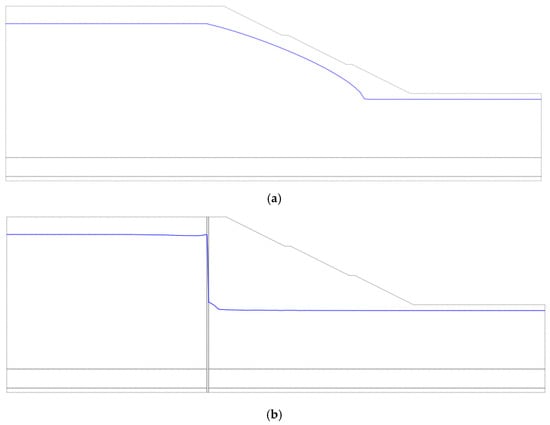
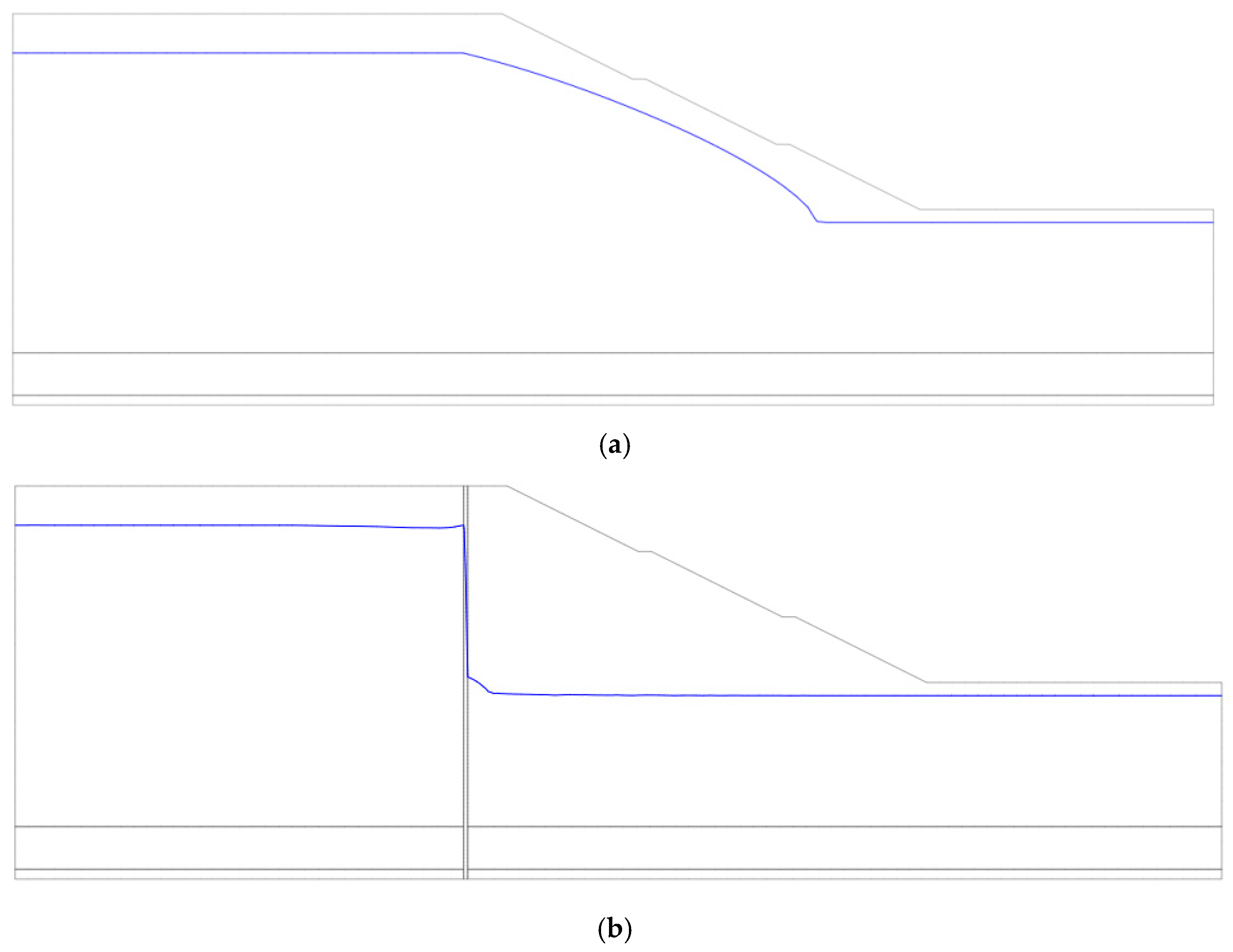
Figure 6.
Phreatic surfaces under groundwater seepage (blue curves) and cutoff wall conditions (vertical black lines). (a) Phreatic surface under non-seepage conditions; (b) phreatic surface and cutoff wall location under cutoff wall conditions.
The finite element mesh, as shown in Figure 5b, comprises 2472 nodes and 2358 elements. The CPE4P quadrilateral elements (4-node bilinear plane strain elements with pore pressure degrees of freedom) were selected for the discretization. These elements inherently support pore pressure degrees of freedom, ensuring full compatibility with Biot’s consolidation theory and the seepage–stress coupling equations without requiring additional simplifications. Furthermore, CPE4P elements demonstrate robust stability in modeling nonlinear materials (e.g., the Mohr–Coulomb constitutive model) and large-deformation scenarios, making them well suited for the geomechanical challenges addressed in this study.
4.2. Validate the Numerical Model
Prior to conducting numerical simulation studies on slope stability, establishing a robust numerical model validation framework proves essential. Field monitoring datasets acquired from actual engineering practice, including deformation measurements of cutoff walls and slope surface displacements, enabled the execution of the first numerical simulation trial using the cutoff wall working condition model. This approach ensures numerical reliability through direct calibration against in situ monitoring evidence, while maintaining strict correspondence between simulation parameters and observed geotechnical behavior.
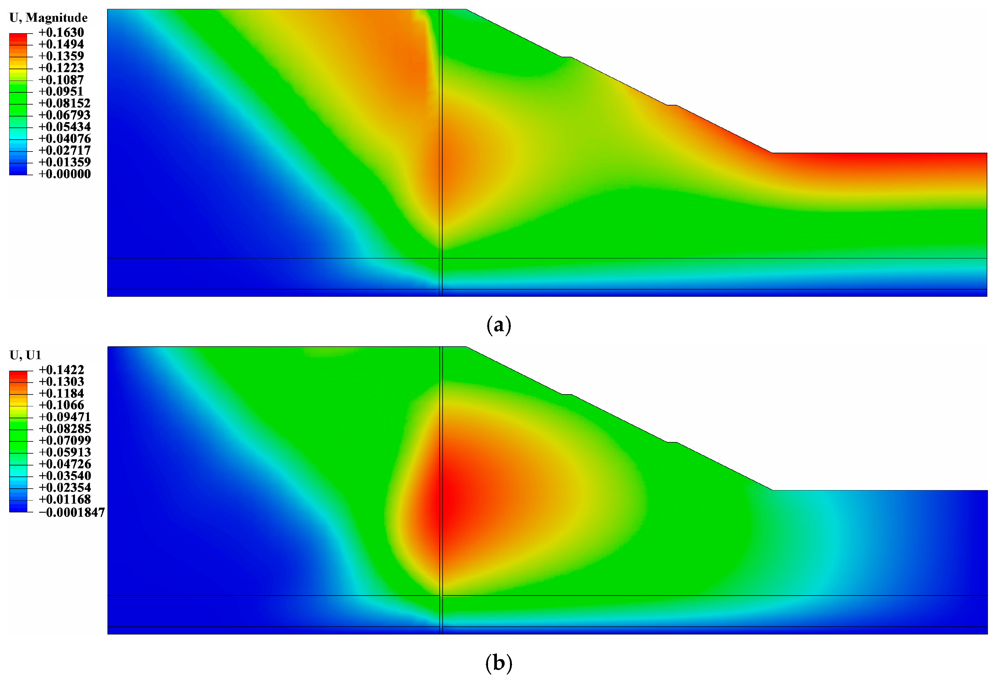
Based on the total displacement (Figure 7a) contour map of the slope, it was observed that the primary displacements occurred at the settlement location on the slope crest, at the position where the cutoff wall endured the maximum hydrostatic pressure, and at the rebound location at the slope toe.
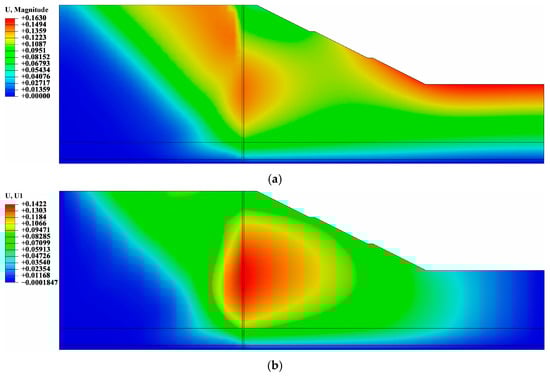
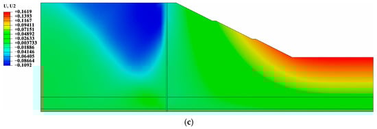
Figure 7.
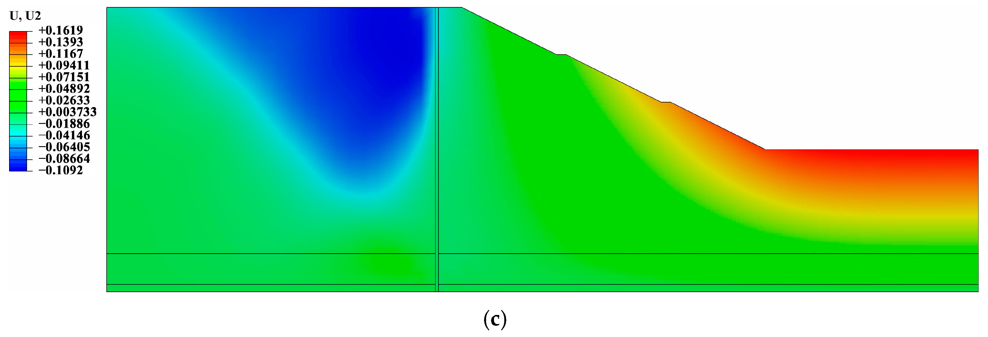
The displacement contour maps of the slope under the cutoff wall conditions. Stratigraphic boundaries are represented by horizontal black lines, and vertical black lines denoting cutoff wall boundaries in these figures. (a) Total displacement; (b) horizontal displacement; (c) vertical displacement.
From the perspective of horizontal displacement (Figure 7b), the maximum horizontal displacement of the slope was detected at the middle segment of the cutoff wall, with the positive direction oriented to the right. The horizontal displacement range was from −0.0008018 m to +0.1422 m. This displacement pattern emerged because the cutoff wall effectively obstructed seepage from the left side of the slope, while on the right side, the phreatic line in the excavated slope matched the post-rainfall water level, resulting in no active seepage. Consequently, the cutoff wall primarily sustained hydrostatic pressure in the horizontal direction. The head difference in the middle segment of the wall was the greatest, leading to maximum hydrostatic pressure and significant horizontal displacement in this region. Additionally, the maximum horizontal displacement on the slope surface occurred in the middle of the slope.
In terms of vertical displacement (Figure 7c), the maximum vertical displacement of the slope was noted at the crest and the toe, with the positive direction upwards. The displacement varied from −0.1092 m to +0.1619 m. Vertical displacement at the slope crest manifested as settlement, while at the slope toe, it appeared as rebound. The primary cause of these vertical displacements was attributed to the alteration of the stress field in the geomaterials during excavation.
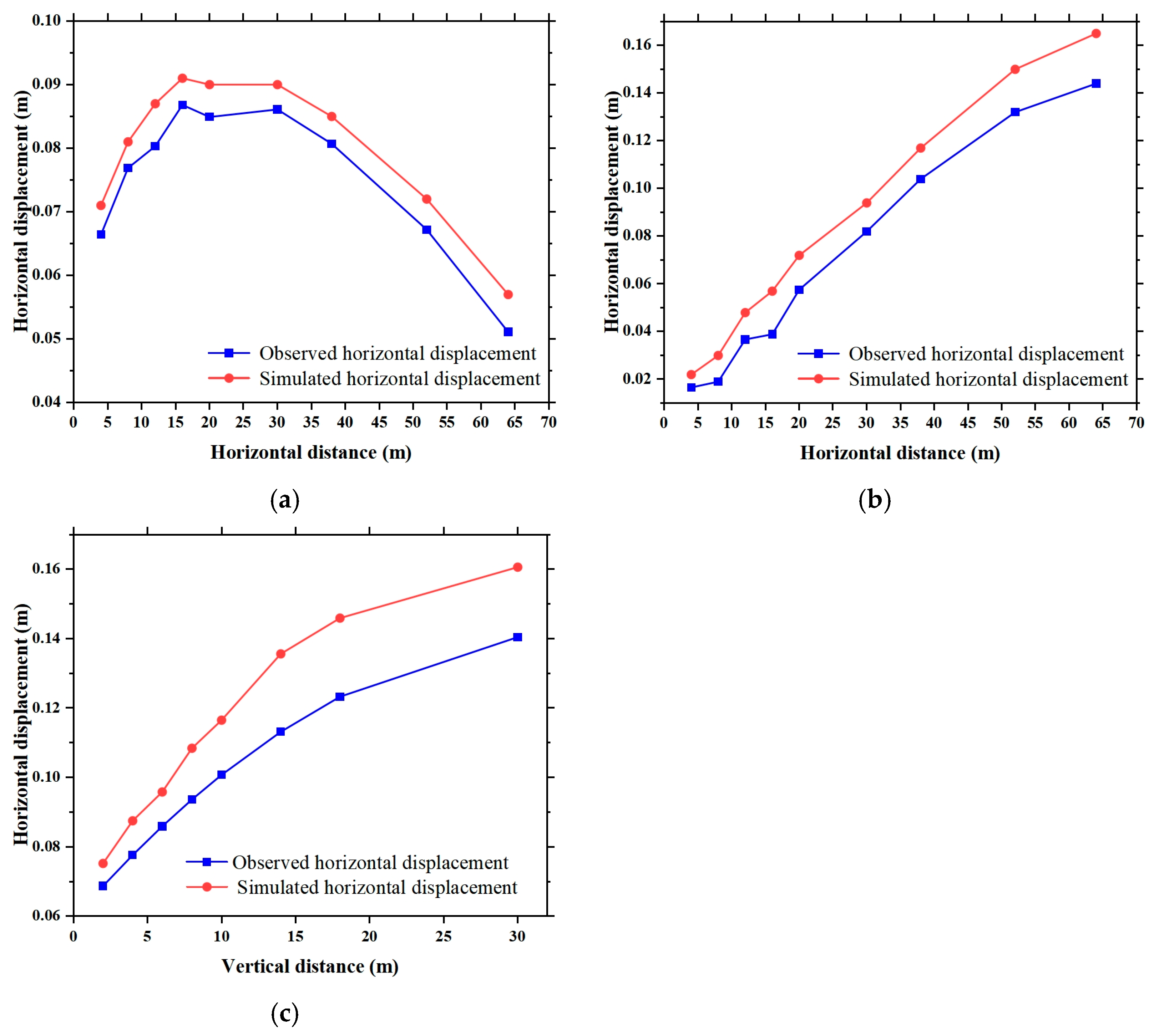
The numerical model was calibrated using field monitoring data from Section 2.2 (slope surface displacements) and Section 2.3 (cutoff wall strains). The observed range of horizontal displacement from the total station was between +0.057 m and +0.091 m. The numerical simulation tests resulted in horizontal displacement ranging from +0.051 m to +0.087 m, which was slightly smaller than the observed data (Figure 8a). The total station data for vertical displacement ranged from +0.022 m to +0.165 m, while the simulation results for vertical displacement ranged from +0.017 m to +0.144 m (Figure 8b). Similar to horizontal displacements, the simulated values for vertical displacements were slightly smaller than the observed values, but the overall trend remained consistent. The strain gauge recorded horizontal displacement of the cutoff wall in the range of +0.0752 m to +0.1606 m, while the simulation yielded a range of +0.0687 m to +0.1404 m (Figure 8c). Consistent with slope displacement, the cutoff wall’s simulated horizontal displacement was slightly less than the observed values, although the overall pattern was similar.
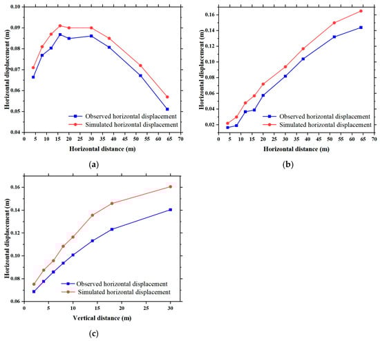
Figure 8.
Comparison of monitoring data and simulation data. (a) Horizontal displacement of the slope surface; (b) vertical displacement of the slope surface; (c) horizontal displacement of the cutoff wall.
These discrepancies are attributable to the focus of this research on the effects of the cutoff wall on slope stability, emphasizing seepage–stress coupling effects while simplifying other conditions such as temperature and wind fields. Furthermore, the Mohr–Coulomb constitutive model was adopted in this simulation, which lacks the capability to describe the nonlinear stress–strain behavior and strain-softening characteristics of soil or rock. It cannot accurately simulate the progressive failure process and residual strength characteristics of materials, nor does it account for dynamic effects like creep, stress relaxation, and seismic impacts on soil strength. While there are certain numerical discrepancies between the monitoring and simulated data, the numerical model exhibits strong qualitative consistency with field observations. Critically, both datasets demonstrate identical deformation trends: vertical displacement concentration at the slope toe due to unloading rebound and horizontal displacement peaking at the mid-depth of the cutoff wall under hydrostatic pressure. These alignments confirm the model’s capability to capture dominant hydromechanical mechanisms.
In conclusion, the numerical model established in this study demonstrated sufficient reliability and effectively reflected actual conditions, indicating its applicability for the numerical simulation tests conducted in this research.
4.3. Analysis of Slope Stability Under Natural Conditions
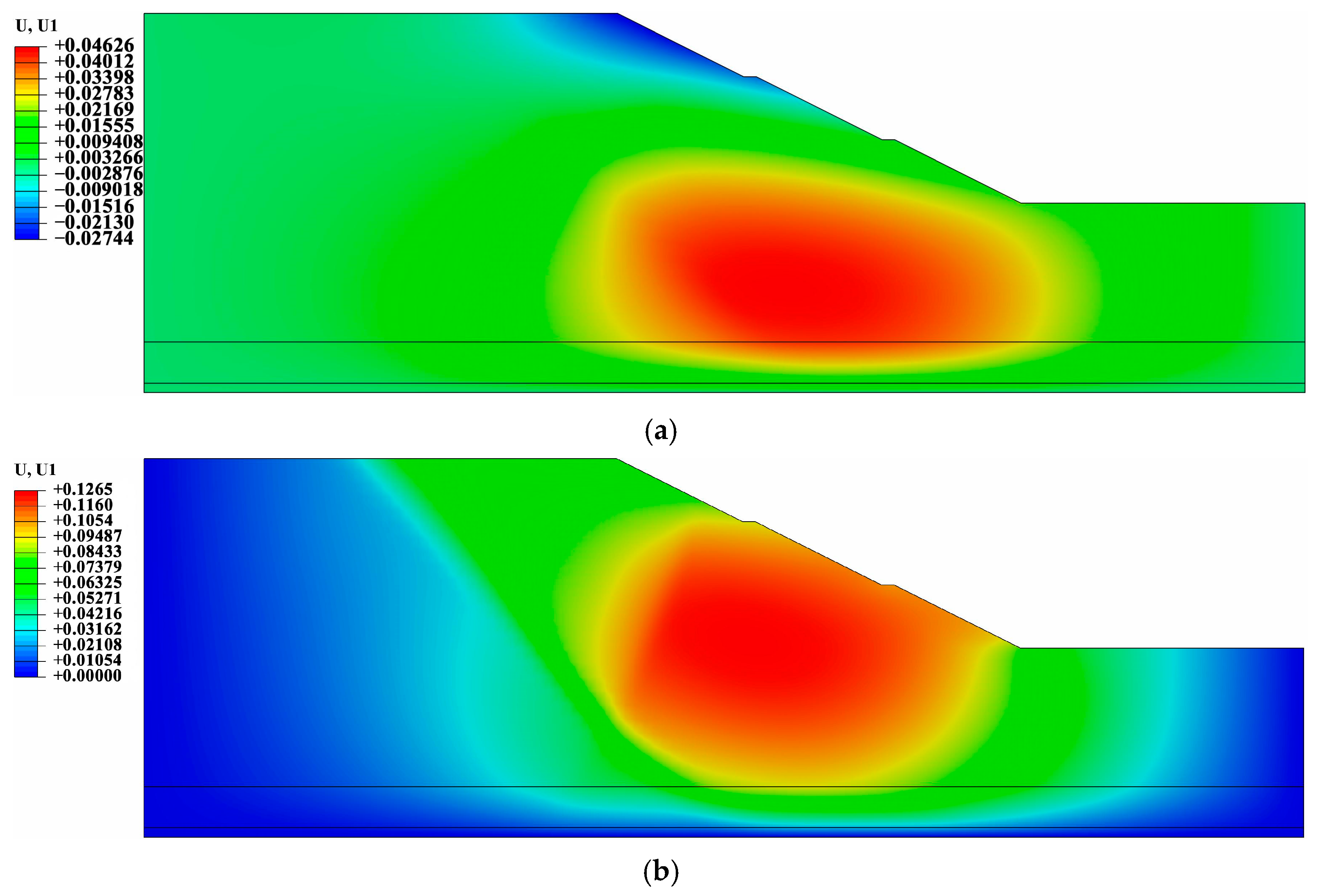
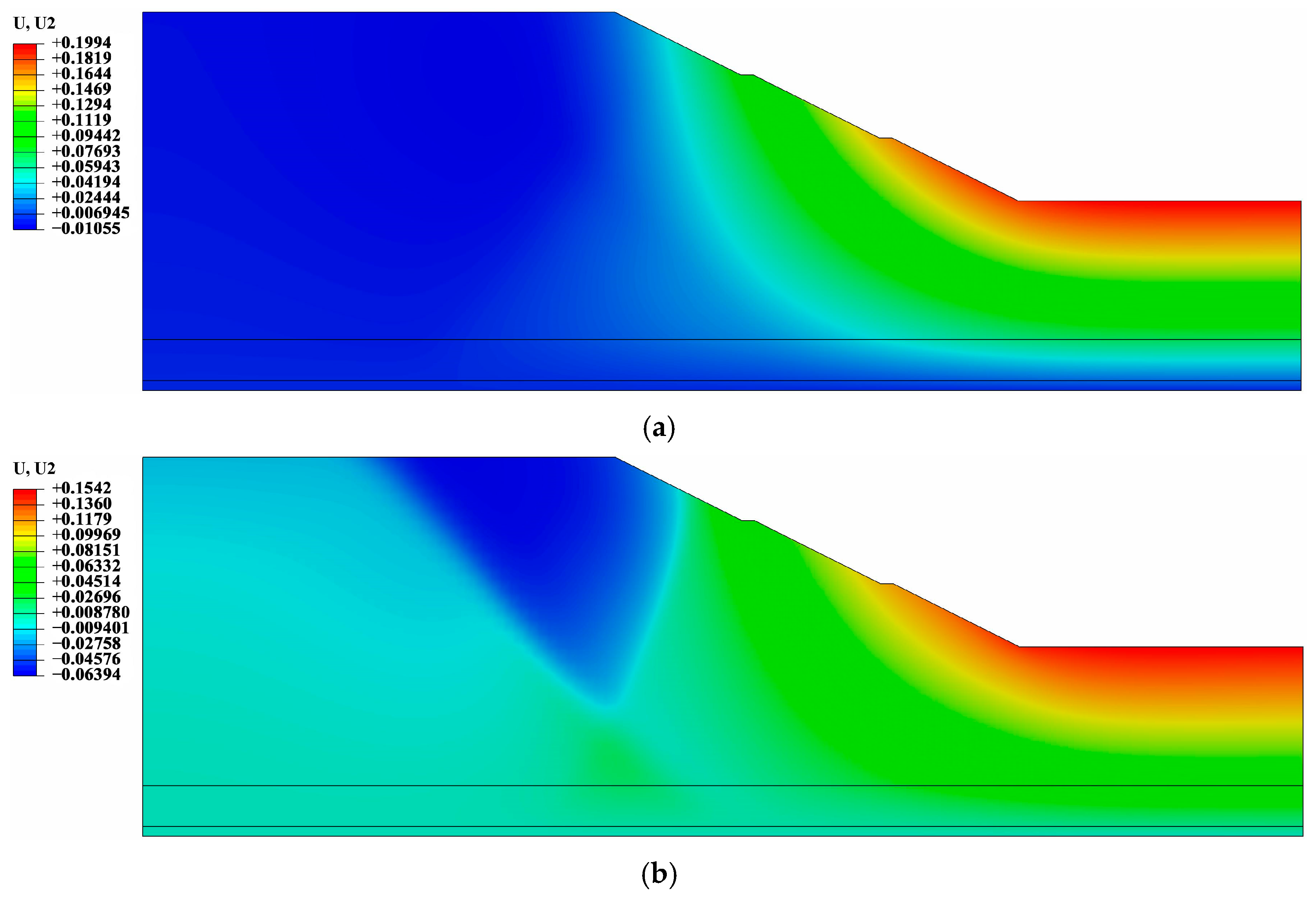
The slope’s horizontal displacement exhibits a distribution range of −0.02744 m to +0.04626 m (Figure 9a). Notably, the maximum horizontal displacement occurs not at the slope surface but near the interface between the sandy cobble gravel layer and sandy clay layer, demonstrating upward propagation characteristics. This phenomenon correlates with interfacial friction effects induced by lithological heterogeneity, where relative slip along deep stratigraphic interfaces in gentle slopes tends to concentrate displacements more significantly than surface movements. Vertical displacement fields display a range of +0.01055 m to +0.1994 m (Figure 10a), with maximum displacements persistently localized at the excavation layer’s toe due to stress redistribution from unloading effects. Numerical simulations reveal that upon completing the fifth excavation stage, potential slip surfaces extend through the lower third of the slope, indicating substantial vertical shear failure risks. The safety factor calculated using the strength reduction method was 1.65, satisfying the 1.25 requirement for temporary slopes specified in the Technical Code for Building Slope Engineering (GB50330-2013). Figure 8 visually documents the potential slip surface morphology under these working conditions.
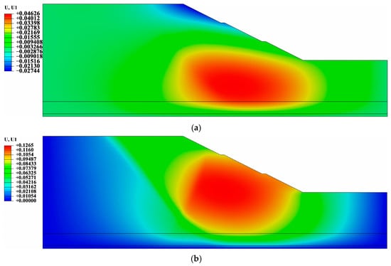
Figure 9.
Comparison of slope horizontal displacement under non-seepage and groundwater seepage conditions, stratigraphic boundaries are represented by horizontal black lines in thses figures. (a) Non-seepage conditions; (b) groundwater seepage conditions.
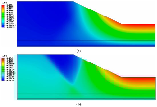
Figure 10.
Comparison of slope vertical displacement under non-seepage and groundwater seepage conditions. (a) Non-seepage conditions; (b) groundwater seepage conditions.
Pore water pressure gradients induce significant alterations in horizontal displacement fields, with maximum values increasing to +0.126 m (Figure 9b) and displacement concentration zones expanding from internal slope regions to ground surfaces. These modifications directly relate to seepage forces generated by water table depression at the slope toe during excavation. Hydraulic gradients amplify lateral deformations in geotechnical materials. Although maximum vertical displacement at the slope toe remains +0.1542 m (Figure 10b), this value decreases by approximately 22.7% compared to non-seepage conditions, indicating altered deformation mechanisms. The recalculated safety factor under seepage conditions reduces to 1.165, representing a 29.4% decrease from the non-seepage scenario. Modified slip surface geometries confirm seepage’s substantial influence on failure patterns. This safety coefficient falls below the 1.25 minimum threshold for temporary slopes, demonstrating insufficient stability under seepage conditions to meet engineering safety standards.
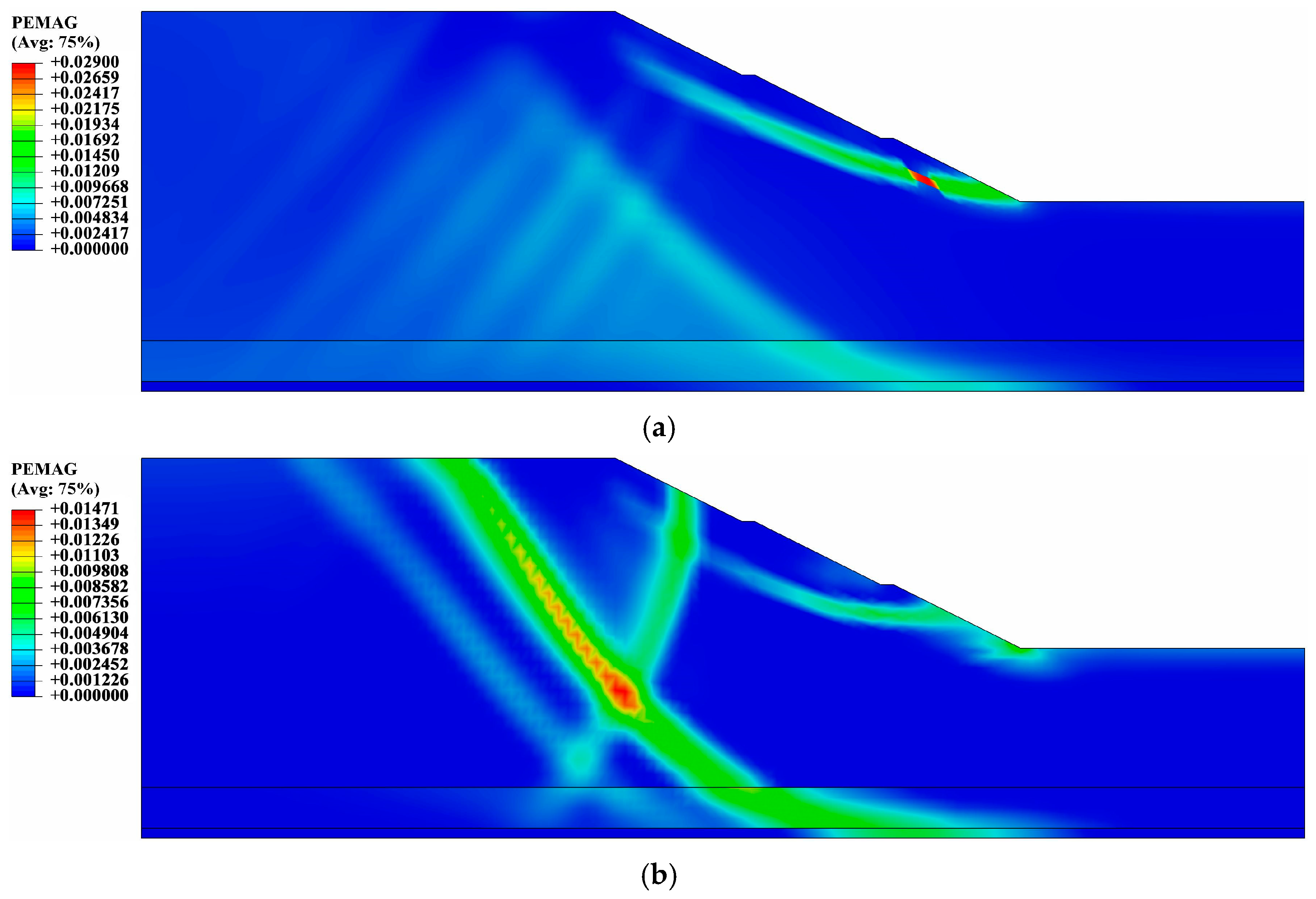
Comparative analysis of both working conditions reveals groundwater’s dual mechanisms affecting slope stability. Non-seepage failure predominantly manifests through vertical shear with relatively higher safety margins (1.65 > 1.25) (Figure 11a), whereas seepage conditions shift failure modes to horizontal shear dominance through stress field modifications. This transition manifests through three quantitative indicators: 173% horizontal displacement increase, over 20% vertical displacement reduction, and nearly 30% safety factor decrease. The 7.2% shortfall between the safety factor under seepage conditions (1.165) (Figure 11b) and the code requirement (1.25) signifies stability transition from “safe” to “critical failure” states. Displacement field evolution further corroborates this conclusion non-seepage slip surfaces remain confined to lower slope regions, while seepage-induced surfaces propagate to ground level, forming complete failure paths. Groundwater seepage ultimately degrades slope stability through multiple pathways: altering pore pressure distributions, weakening geotechnical shear strength, and intensifying stress redistribution effects.
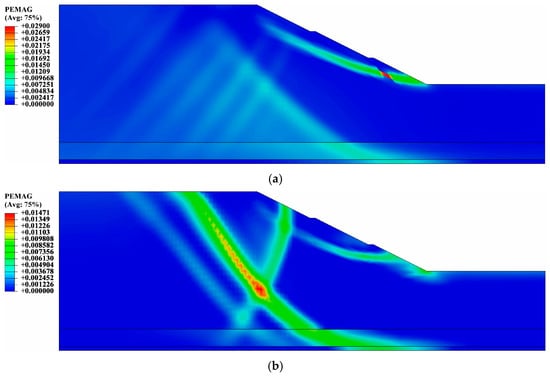
Figure 11.
Comparison of slope potential slip surfaces under non-seepage and groundwater seepage conditions (a) Non-seepage conditions [safety factor (FS) = 1.650]; (b) groundwater seepage conditions (FS = 1.165).
4.4. Selection of the Optimal Slope Ratio Under Natural Conditions
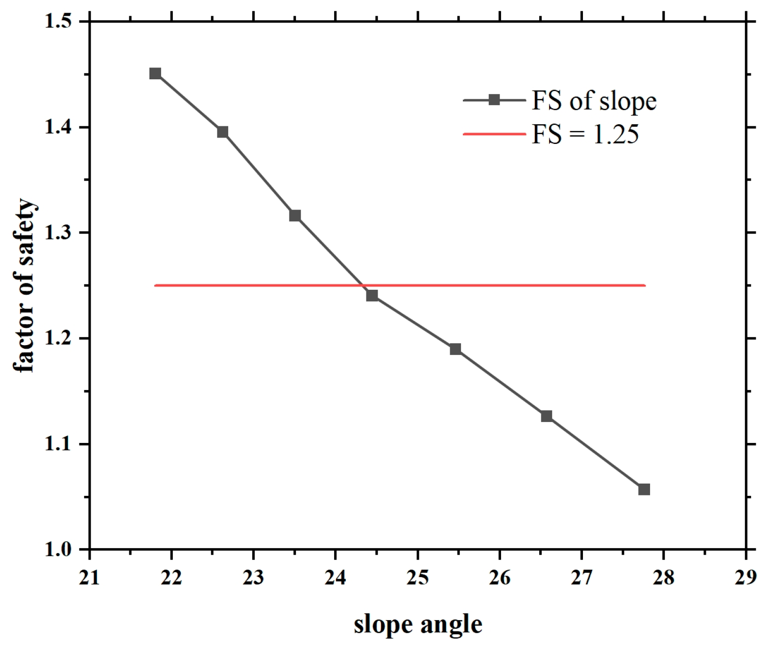
Numerical modeling was employed to simulate natural slope behavior under seepage–stress coupling conditions. Analyses encompassed slope ratios ranging from 1:2.5 to 1:1.9, corresponding to slope angles between 21.80° and 27.76°. The results demonstrate a monotonic decrease in safety factors with increasing slope angles. Numerical simulations identified 24.33° (Figure 12) as the optimal slope angle under natural conditions, equivalent to a slope ratio of approximately 1:2.21, where stability requirements and geometric efficiency achieve balanced optimization.
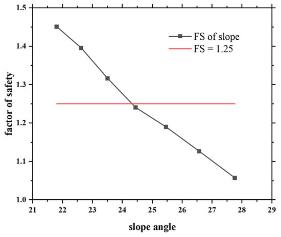
Figure 12.
The relationship curve between the FS of the slope under natural conditions and the slope angle.
4.5. Slope Stability Analysis Under the Conditions of Cutoff Wall
Under natural conditions, the safety factor of the slope was only 1.165 when a slope ratio of 1:2.0 was selected. This value was below the minimum requirement for the safety factor of a temporary slope. Therefore, in actual engineering practice, a cutoff wall was implemented as a reinforcement measure to enhance the safety and stability of the slope by effectively mitigating the impact of seepage. This design strategy aimed to improve the overall stability of the slope structure, ensuring safety during construction and usage while minimizing potential engineering risks.
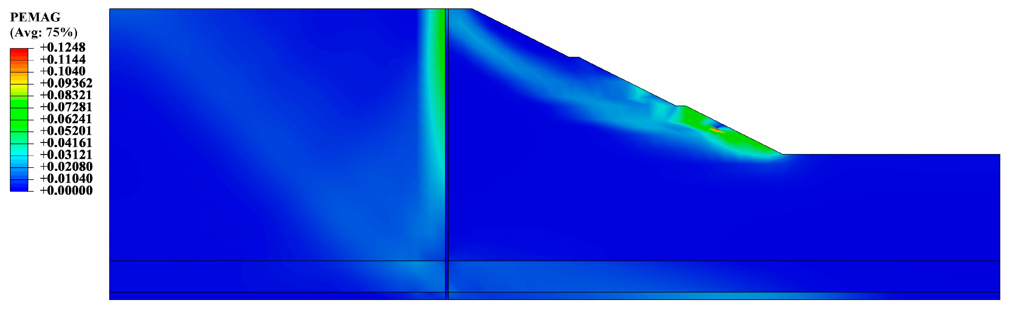
According to the results of numerical simulations, the safety factor of the slope upon completion of excavation with the cutoff wall in place was 1.653. Figure 13 depicts the potential sliding surface under this condition. At this point, the safety factor of the slope significantly exceeded the prescribed value of 1.25 for temporary slopes, indicating strong slope stability. The displacement cloud diagram of the slope under this condition is shown in Figure 7.
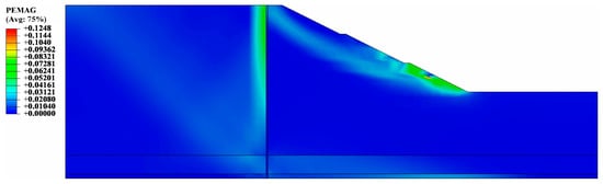
Figure 13.
Potential sliding surface of the slope under cutoff wall conditions (FS = 1.653).
4.6. Selection of Optimal Slope Ratio Under Cutoff Wall Conditions
Numerical simulation results from this study determined the safety factor of a cutoff wall-reinforced slope at 1:2.0 ratio as 1.653 in actual engineering applications, significantly exceeding the 1.25 standard requirement. To enhance cost-effectiveness in future similar projects, this study systematically investigated optimal slope ratios under cutoff wall conditions through parametric analysis.
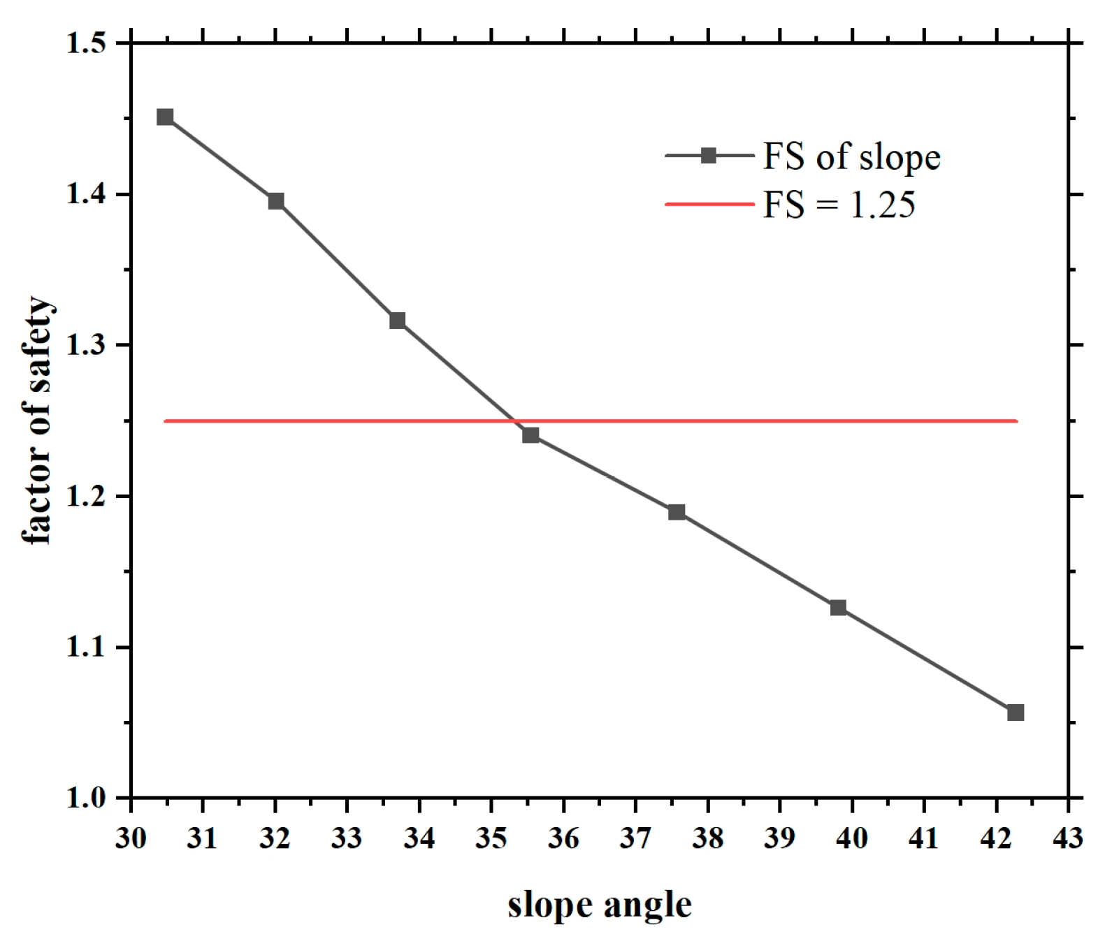
The stability evaluation encompassed slope ratios from 1:1.7 to 1:1.1, corresponding to slope angles between 30.47° and 42.27°, with safety factors demonstrating monotonic increase as slope gradients decreased. Numerical simulations identified 35.31° as the optimal slope angle under cutoff wall conditions, equivalent to a slope ratio of 1:1.41 (Figure 14).
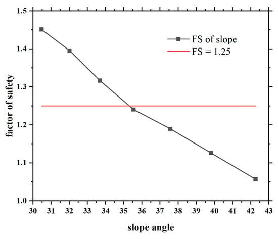
Figure 14.
The relationship curve between slope safety factor and slope angle under cutoff wall conditions.
4.7. Comparative Analysis of Optimal Slope Ratios and Economic Benefits
Under natural seepage conditions, the optimal slope angle of 24.33° (equivalent to a slope ratio of 1:2.21) requires an excavation volume per unit width of 1989 m3/m (Table 2), calculated as a trapezoidal cross-section with a vertical depth of 30 m and horizontal length of 66.3 m. Implementing a cutoff wall increases the optimal slope angle to 35.31° (slope ratio 1:1.41), reducing the horizontal excavation length to 42.3 m and lowering the excavation volume per unit width to 1269 m3/m. This results in a 36.2% reduction in earthwork volume, directly translating to decreased material removal costs and accelerated construction timelines. The steeper slope enabled by the cutoff wall demonstrates significant technical and economic advantages, aligning with geotechnical optimization principles for deep excavations in permeable geological settings.
Table 2.
Comparison of optimal slope angles, ratios, and excavation volume reduction.
5. Discussion
5.1. Variation in Slope Stability with Changes in the Strength of the Cutoff Wall
The implementation of cutoff walls increased the slope safety factor from 1.165 to 1.653 under a 1:2.0 slope ratio, while the optimal slope ratio improved from 1:2.21 to 1:1.41. This enhancement clearly demonstrates the effectiveness of cutoff walls in controlling internal seepage mechanisms, thereby significantly improving slope stability. Consequently, this study further investigates the influence of key cutoff wall parameters on safety factors through systematic parametric analysis.
The elastic modulus of cutoff walls constitutes a critical design parameter. The original design specified a wall strength of 2.5 MPa with an elastic modulus of 7403 MPa. To evaluate the mechanical performance dependence on material stiffness, numerical simulations incorporated elastic modulus values ranging from 7000 MPa to 12,000 MPa while maintaining constant geotechnical parameters, ensuring isolated analysis of modulus effects.
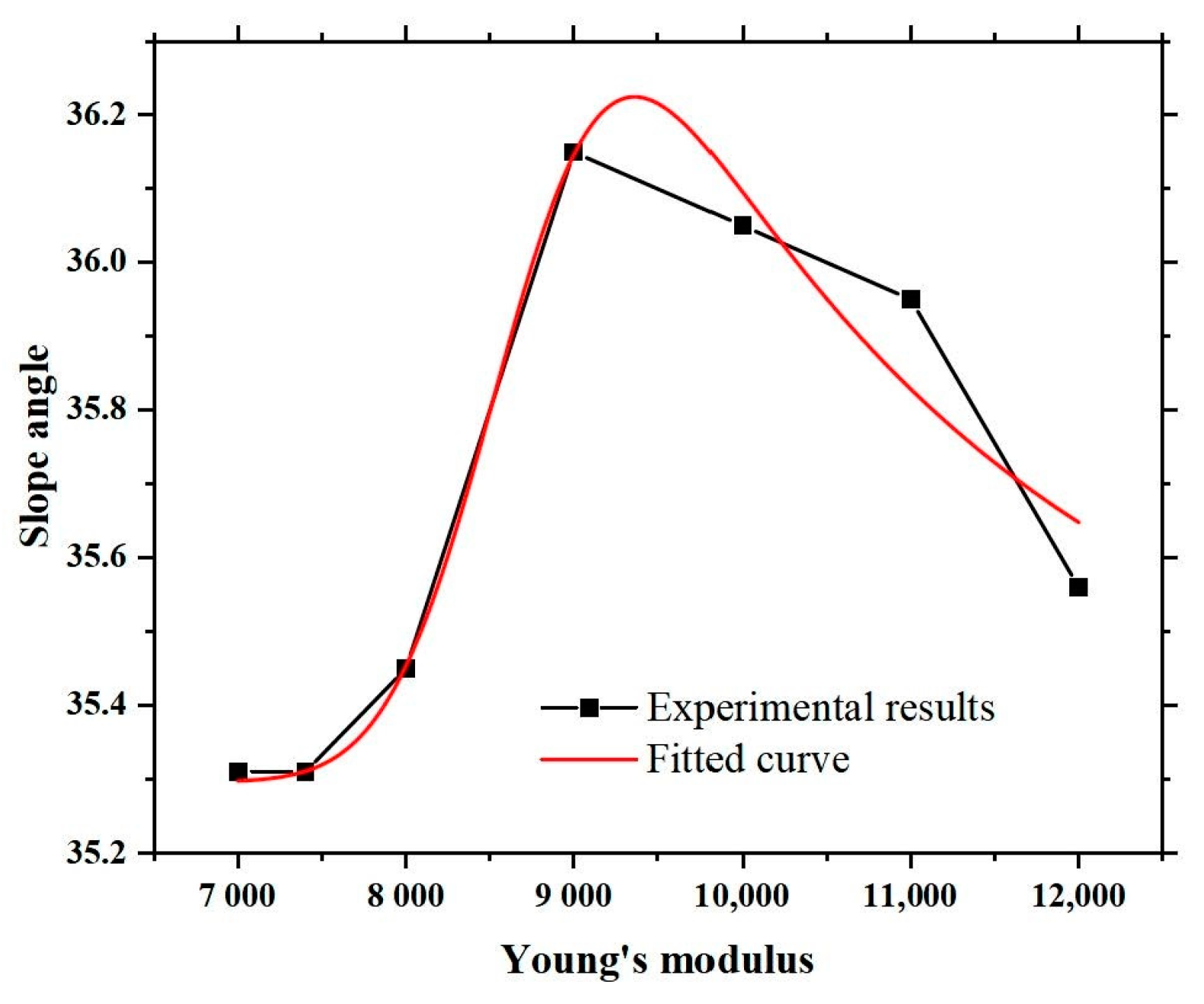
Optimal slope angles exhibit modulus-dependent characteristics (Figure 15). When Young’s modulus remains below 9000 MPa, increasing rigidity enhances retaining capacity, resulting in progressive elevation of optimal slope angles. However, exceeding 9000 MPa induces excessive stiffness mismatch between the wall and surrounding soils, triggering brittle failure mechanisms due to incompatible deformation patterns. Consequently, optimal angles decrease beyond this threshold. Based on these findings, the optimal Young’s modulus range for cutoff walls is determined to be 8000–10,000 MPa. The fitting equation is expressed as follows:
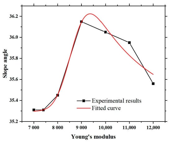
Figure 15.
Relationship between Young’s modulus of cutoff walls and optimal slope angles.
Based on the fitting equation, the maximum slope angle of 36.20° was achieved at a Young’s modulus of 9362.82 MPa for the cutoff wall, corresponding to an optimal slope ratio of 1:1.37.
5.2. Variation in Slope Stability with Changes in the Thickness of the Cutoff Wall
Wall thickness constitutes a critical parameter in cutoff wall design. Given potential difficulties in precisely controlling Young’s modulus during construction, this study investigates the economic implications of thickness variation while maintaining slope stability. Numerical simulations evaluated thickness effects across 0.1–1.0 m ranges under constant parameters, with the original design thickness being 0.6 m.
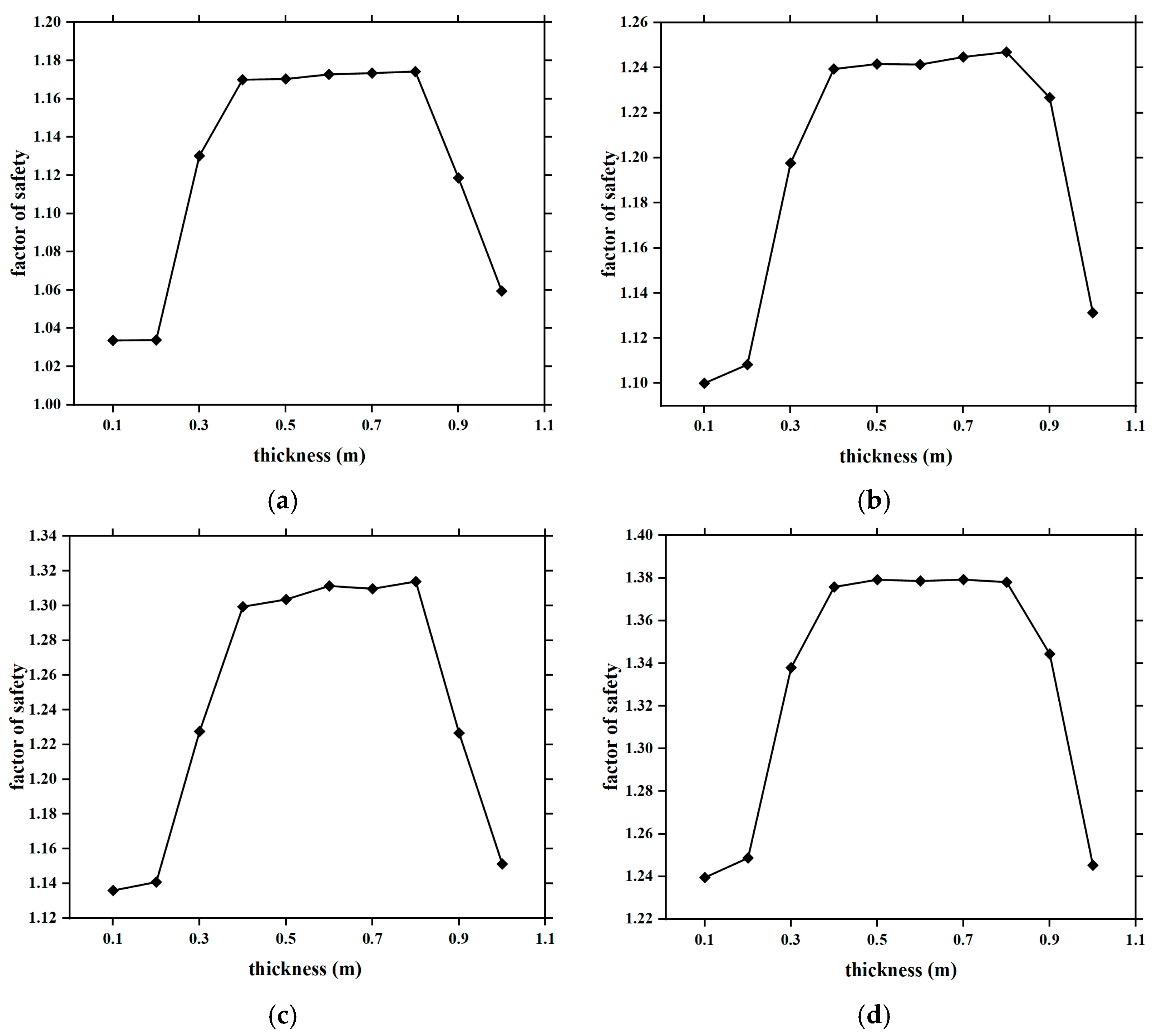
Tests conducted on slopes with 1:1.3, 1:1.4 1:1.5 and 1:1.6 ratios revealed distinct thickness-dependent stability patterns (Figure 16). Within the 0.4–0.8 m range, safety factors exhibited marginal increases (≤2%) with thickness growth, attributed to enhanced seepage control capacity and partial retaining wall functionality. Below 0.3 m, safety factors decreased exponentially (15–22% reduction), suggesting hydraulic breakthrough risks in ultra-thin walls. Conversely, thicknesses exceeding 0.9 m caused abrupt safety factor declines (18–25%), indicative of brittle failure susceptibility in over-thick configurations. This phenomenon arises from the significant stiffness contrast between the excessively thick cutoff wall and the surrounding high-permeability sandy gravel layer, which prevents stress relief through coordinated deformation and further amplifies risks of shear crack propagation and hydraulic fracturing.
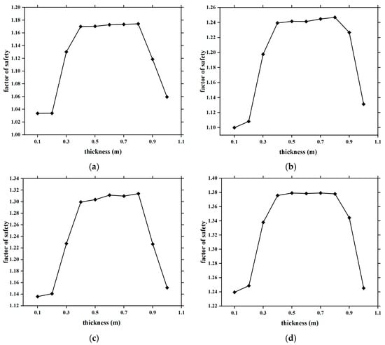
Figure 16.
Effect of variation in thickness of the cutoff wall on slope stability. (a) The slope ratio is 1:1.3; (b) the slope ratio is 1:1.4; (c) the slope ratio is 1:1.5; (d) the slope ratio is 1:1.6.
Economic analysis demonstrated that reducing wall thickness from 0.6 m to 0.4–0.5 m maintains safety factor variations within ±1% while achieving 16.7–33.3% concrete savings. This optimization strategy effectively balances technical requirements with material efficiency, particularly valuable in large-scale projects with extensive cutoff wall applications.
5.3. Model Limitations
This section critically evaluates the limitations of the numerical framework and assumptions adopted in this study, providing insights into potential areas for methodological refinement in future research.
5.3.1. The Simplified Constitutive Model
The Mohr–Coulomb model, while widely used, cannot capture nonlinear stress–strain behaviors, strain-softening effects, or residual strength characteristics of soils. This simplification may underestimate progressive failure mechanisms in highly heterogeneous or fissured geological formations.
5.3.2. The Static Analysis Framework
The model assumes static loading conditions and ignores dynamic effects such as seismic activity, vibration from adjacent construction, or long-term creep deformation, limiting its applicability to seismically active regions or projects requiring long-term stability assessments.
5.3.3. The Homogeneous Material Assumptions
Stratigraphic layers were treated as homogeneous isotropic media. In reality, spatial variability in permeability, localized fractures, or boulder inclusions could induce unmodeled stress concentrations or preferential seepage paths.
6. Conclusions
This study investigates the deep excavation slope of an intake box culvert in a water diversion project located in western Yunnan Province. The numerical model was validated using field monitoring data and employed to analyze post-excavation stability under three working conditions: non-seepage, groundwater seepage, and cutoff wall implementation. Parameter optimization strategies for cutoff walls were subsequently proposed based on analytical findings. The following results were obtained:
- Groundwater seepage reduces the safety factor of natural slopes by 29.4%, decreasing it from 1.65 to 1.165, primarily due to pore pressure redistribution and horizontal shear failure mechanisms. This underscores the necessity of integrating hydromechanical coupling effects in slope design for permeable geological settings.
- Implementing cutoff walls increases the optimal slope ratio from 1:2.21 with a safety factor of 1.165 to 1:1.41 with a safety factor of 1.653, achieving a 36.2% reduction in excavation volume, decreasing it from 1989 to 1269 m3/m per unit width. This demonstrates the dual techno–economic benefit of cutoff walls in balancing stability and cost efficiency.
- For the cutoff wall, a critical Young’s modulus threshold of 9362.63 MPa maximizes the slope angle to 35.31°, corresponding to a slope ratio of 1:1.37. Beyond this threshold, excessive stiffness significantly amplifies the risk of brittle failure due to stiffness incompatibility with the surrounding soils, highlighting the necessity of stiffness compatibility between the wall and surrounding soils.
- Reducing the cutoff wall thickness from 0.6 m to 0.4 m ensures compliance with safety standards and achieves 33% concrete savings. This provides actionable guidelines for material-efficient designs in large-scale projects.
This study demonstrates that optimized cutoff walls enhance slope stability while advancing sustainability through minimized ecological disruption and resource-efficient design. By integrating stiffness-compatible parametric analysis with environmental preservation principles, these findings provide actionable insights for implementing eco-conscious geotechnical practices in deep excavation projects, aligning infrastructure development with global sustainability goals.
Author Contributions
Conceptualization, F.L., Z.L. and Z.K.; methodology, F.L., Z.L. and Z.K.; software, F.L.; validation, F.L., Z.L. and Z.K.; formal analysis, F.L., H.C. and Z.C.; investigation, F.L. and Z.L.; resources, Z.L. and Z.K.; data curation, H.C., Z.K. and Z.L.; writing—original draft preparation, F.L.; writing—review and editing, F.L., Z.L. and Z.K.; visualization, F.L.; supervision, H.C. and Z.C.; project administration, H.C. and Z.K.; funding acquisition, Z.L. All authors have read and agreed to the published version of the manuscript.
Funding
This research was funded by the science and technology development project of Sinohydro Foundation Engineering Co., Ltd. (Tianjin, China). Evaluation of the rapid excavation of the slope cutoff wall in the complex geological background area and treatment technology of mud and water inrush in tunnel engineering (Grant No. 2022530103001936).
Institutional Review Board Statement
Not applicable.
Informed Consent Statement
Not applicable.
Data Availability Statement
The data of experimental in this paper are available upon request from the author.
Acknowledgments
We are also sincerely thankful to the editors and reviewers for reviewing papers. We are very grateful to our colleagues on the team who supported the implementation of this project.
Conflicts of Interest
The authors declare no conflicts of interest.
References
- Luo, X.Q.; Liu, D.F.; Wu, J.; Cheng, S.G.; Shen, H.; Xu, K.X.; Huang, X.B. Model test study on landslide under rainfall and reservoir water fluctuation. Chin. J. Rock Mech. Eng. 2005, 24, 2476–2483. [Google Scholar]
- Xie, L.F.; Duan, X.B. Experiment Study on Slope Stability under Unsteady Seepage. J. Yangtze River Sci. Res. Inst. 2009, 26, 31–34. [Google Scholar]
- He, L.L.; Zhou, L.; Liang, Y. Simplified analysis method for the bank slope stability with the influence of water level plummet. Hydro-Sci. Eng. 2021, 43, 16–24. [Google Scholar]
- Chu, W.J.; Xu, W.Y.; Su, J.B. Study on solid-fluid-coupled model and numerical simulation for deformation porous media. Eng. Mech. 2007, 24, 56–64. [Google Scholar]
- Liu, Q.S.; Li, J.L.; Liu, B. Hydromechanical coupling model for clay of nuclear waste repository based on percolation theory. Disaster Adv. 2013, 6, 33–37. [Google Scholar]
- Li, H.; Tian, H.Y.; Ma, K. Seepage characteristics and its control mechanism of rock mass in high-steep slopes. Processes 2019, 7, 71. [Google Scholar] [CrossRef]
- Khurshid, M.N.; Khan, A.H.; Rehman, Z.U.; Chaudhary, T.S. The evaluation of rock mass characteristics against seepage for sustainable infrastructure development. Sustainability 2022, 14, 10109. [Google Scholar] [CrossRef]
- Kiriakidis, L.; Constantino, R. Seepage in Earth Slopes with Longitudinal Drainage Trenches. Master’s Thesis, West Virginia University, Morgantown, WV, USA, 2002. Available online: https://www.proquest.com/docview/56304520 (accessed on 23 May 2023).
- Cao, H.; Wu, H.F.; Zhang, T.; Yu, H.Y. Experimental Analysis on Relief Wells in Shijiao Section of Beijiang Dike. J. Yangtze River Sci. Res. Inst. 2004, 21, 53–56. [Google Scholar]
- Li, J.J.; Yang, Y.; Duan, X.B.; Xie, L.F.; Zhou, X. Numerical Analysis on Factors Affecting the Effectiveness of Relief-well. J. Yangtze River Sci. Res. Inst. 2016, 33, 151–154. [Google Scholar]
- Xu, W.B.; Yao, Q.H.; Wang, S.; Wu, M.Z. Transient seepage analysis of Beijiang levee and simulation of anti-seepage effect of decompression well. Acta Sci. Nat. Univ. Sunyatseni 2019, 58, 97–103. [Google Scholar]
- Armanuos, A.M.; Negm, A.M.; Javadi, A.A.; Abraham, J.; Gado, T.A. Impact of inclined double-cutoff walls under hydraulic structures on uplift forces, seepage discharge and exit hydraulic gradient. Ain Shams Eng. J. 2022, 13, 101531. [Google Scholar] [CrossRef]
- Huang, Z.X.; Shen, Z.Z.; Xu, L.Q.; Sun, Y.Q.; Li, H.X.; Liu, D.T. Seepage characteristics of core rockfill dam foundation with double cutoff walls in deep overburden: A case study. Case Stud. Constr. Mater. 2024, 21, e03576. [Google Scholar] [CrossRef]
- Farouk, M. Controlling seepage flow beneath hydraulic structures: Effects of floor openings and sheet pile wall cracks. Buildings 2024, 14, 2234. [Google Scholar] [CrossRef]
- Sugawara, K.; Matsumura, Y.; Ashitaka, Y.; Tominaga, S.; Kaneda, M. Effects of wall permeability on turbulence. Int. J. Heat Fluid Flow 2010, 31, 974–984. [Google Scholar] [CrossRef]
- Hartog, F.H.; van Nesselrooij, M.; van Campenhout, O.W.G.; Schrijer, F.F.J.; van Oudheusden, B.W.; Masania, K. Turbulent boundary layers over substrates with streamwise-preferential permeability. Phys. Rev. Fluids 2024, 9, 114602. [Google Scholar] [CrossRef]
- Biniyaz, A.; Azmoon, B.; Liu, Z. Coupled transient saturated-unsaturated seepage and limit equilibrium analysis for slopes: Influence of rapid water level changes. Acta Geote. 2022, 17, 2139–2156. [Google Scholar] [CrossRef]
- Huang, M.S.; Li, Y.S.; Shi, Z.H.; Lu, X.L. Face Stability Analysis of Shallow Shield Tunneling in Layered Ground Under Seepage Flow. Tunn. Undergr. Space Technol. 2022, 119, 104201. [Google Scholar] [CrossRef]
- Zhou, X.P.; Wei, X.; Liu, C.; Cheng, H. Three-Dimensional Stability Analysis of Bank Slopes with Reservoir Drawdown Based on Rigorous Limit Equilibrium Method. Int. J. Geomech. 2020, 20, 04020229. [Google Scholar] [CrossRef]
- Griffiths, D.V.; Lane, P.A. Slope stability analysis by finite elements. Géotechnique 1999, 49, 387–403. [Google Scholar] [CrossRef]
- Zheng, Z.; Xu, H.Y.; Wang, W.; Zhang, Q.; Wang, Y.J.; Sun, Q.C.; Tao, H.H.; Han, X.F. Seepage-Stress Combined Experiment and Damage Model of Rock in Different Loading and Unloading Paths. Int. J. Damage Mech. 2024, 33, 3–38. [Google Scholar] [CrossRef]
- Chai, H.B.; Cao, P.; Lin, H.; Zhao, Y.L. Criteria of elastic strain energy in slope stability analysis using strength reduction method. J. Cent. South Univ. Sci. Technol. 2009, 40, 1054–1058. [Google Scholar]
- Jin, X.G.; Chen, L.H.; Zhang, Y.X. Application of FEM strength reduction method to geotechnical engineering with the consideration of tension and shear failures. J. Chongqing Univ. 2013, 36, 97–104. [Google Scholar]
- Chen, Z.Y.; Song, Y.H.; Yan, H.; Chen, K.D. Analyses of the existing problems in the double parameters reduction method. Hydrogeol. Eng. Geol. 2019, 46, 125–132. [Google Scholar]
- Zhang, D.M.; He, H.F.; Chen, J.; Wang, Y.Z. Simulation Analysis of Slope Stability Based on Strength Reduction. In Proceedings of the International Conference on Chemical, Material and Metallurgical Engineering (ICCMME 2011), Beihai, China, 23–25 December 2011. [Google Scholar] [CrossRef]
- Viggiani, G.; Tamagnini, C. Ground movements around excavations in granular soils: A few remarks on the influence of the constitutive assumptions on FE predictions. Mech. Cohesive-Frict. Mater. 2000, 5, 399–423. [Google Scholar] [CrossRef]
- Cattoni, E.; Tamagnini, C. On the seismic response of a propped r.c. diaphragm wall in a saturated clay. Acta Geotechnica 2020, 15, 847–865. [Google Scholar] [CrossRef]
- Medawela, S.; Indraratna, B.; Athuraliya, S. Acidic flow-induced clogging of permeable reactive barriers in pyritic terrain. In Proceedings of the GeoCongress on State of the Art and Practice in Geotechnical Engineering (Geo-Congress 2022), Charlotte, NC, USA, 20–23 March 2022; pp. 39–49. [Google Scholar]
- Zang, Y.G.; Yu, B.W.; Jiang, Y.H.; Shang, C.J.; Lian, X.Y.; Jia, Y.F. A simulation-optimization integrated framework for subsurface air barrier strategies to mitigate seawater intrusion in a 3D coastal aquifer. J. Hydrol. 2023, 626, 130307. [Google Scholar] [CrossRef]
- Wang, C.Q.; Yao, J.; Wang, X.Y.; Huang, Z.Q.; Xu, Q.; Liu, F.G.; Yang, Y.F. Pore structure and permeability evolution of porous media under in situ stress and pore pressure: Discrete element method simulation on digital core. J. Porous Media 2024, 27, 45–75. [Google Scholar] [CrossRef]
- Hou, X.P.; Fan, H.H. Study on rainfall infiltration characteristics of unsaturated fractured soil based on COMSOL Multiphysics. Rock Soil Mech. 2022, 43, 563–572. [Google Scholar]
- Kurnaz, T.F.; Erden, C.; Kökçam, A.H.; Dagdeviren, U.; Demir, A.S. A hyper parameterized artificial neural network approach for prediction of the factor of safety against liquefaction. Eng. Geol. 2023, 319, 107109. [Google Scholar] [CrossRef]
- Fu, X.L.; Ni, H.; Zhou, A.N.; Jiang, Z.Y.; Jiang, N.J.; Du, Y.J. An integrated fuzzy AHP and fuzzy TOPSIS approach for screening backfill materials for contaminant containment in slurry trench cutoff walls. J. Clean. Prod. 2023, 419, 138242. [Google Scholar] [CrossRef]
- Osborne, D.M.; Armacost, R.L. State of the art in multiple response surface methodology. In Proceedings of the 1997 IEEE International Conference on Systems, Man, and Cybernetics-Computational Cybernetics and Simulation (SMC 97), IEEE Systems, Man, and Cybernetics Society, Orlando, FL, USA, 12–15 October 1997; pp. 3833–3838. [Google Scholar]
- Zhao, J.; Duan, X.R.; Ma, L.N.; Zhang, J.; Huang, H.W. Importance sampling for system reliability analysis of soil slopes based on shear strength reduction. Georisk Assess. Manag. Risk Eng. Syst. Geohazards 2021, 15, 287–298. [Google Scholar] [CrossRef]
- Hu, C.; Lei, R.D.; Gu, Q.H. Application of Supplementary Sampling Method in Slope Reliability Analysis. Int. J. Geomech. 2023, 23, 04023097. [Google Scholar] [CrossRef]
- Li, D.Q. Effect of driven pile bearing capacity determination methods on safety factors. Rock Soil Mech. 2006, 27, 1733–1738. [Google Scholar]
- Bian, X.Y.; Zheng, J.J.; Xu, Z.J. Reliability design of resistance factor and safety factor for pile groups foundation. J. Huazhong Univ. Sci. Technol. (Nat. Sci.) 2014, 42, 87–91. [Google Scholar]
- Chen, D.W. Coupled Stiffness-Permeability Analysis of a Single Rough Surfaced Fracture by the Three-Dimensional Boundary Element Method. Ph.D. Thesis, University of California, Berkeley, CA, USA, 1990. [Google Scholar]
- Wang, Y. Fracture simulation based on large hydraulic fracturing experiment system in laboratory. Prog. Geophys. 2017, 32, 408–413. [Google Scholar]
- Wang, Y.; Wang, H.M.; Zhu, H.B. Preliminary study on physical experimental simulation of hydraulic fracturing. Prog. Geophys. 2021, 36, 1130–1137. [Google Scholar]
- Zhang, B.H.; Zhou, Y.; Wang, Y.; Hu, X.; Zhou, C. Study on Hydraulic Fracture Propagation and Mechanism of Double Wellbore Experiment in Shale. Chin. J. Undergr. Space Eng. 2022, 18, 1588–1593. [Google Scholar]
- Liu, H.; Zhu, P.P.; Liu, Q.S.; Sun, C.Y.; Yang, Y.T.; He, G.C.; He, C.C. Equivalent nodal intensity-based contact model for 3D finite-discrete element method in rock fracturing analysis. Rock Mech. Rock Eng. 2025, 58, 1–28. [Google Scholar] [CrossRef]


Disclaimer/Publisher’s Note: The statements, opinions and data contained in all publications are solely those of the individual author(s) and contributor(s) and not of MDPI and/or the editor(s). MDPI and/or the editor(s) disclaim responsibility for any injury to people or property resulting from any ideas, methods, instructions or products referred to in the content. |
© 2025 by the authors. Licensee MDPI, Basel, Switzerland. This article is an open access article distributed under the terms and conditions of the Creative Commons Attribution (CC BY) license (https://creativecommons.org/licenses/by/4.0/).