1. Introduction
As a natural resource, daylight has been utilized in simple ways for many years. Daylighting requires the correct placement of openings or apertures in a building envelope to allow light penetration while providing adequate light distribution and diffusion. Conventional daylighting strategies are disadvantageous because many areas, such as storerooms, basements, and corridors are not reached [
1,
2]. At present, the use of natural light has developed as a new technology to reduce both energy consumption and cost. As a part of solar energy, solar light delivers excessive thermal gains and brightness into any building interior because of the embodied energy of direct sunlight [
3].
Natural light technology has recently demonstrated some notable achievements, such as providing high-quality lighting, as well as highly efficient and, sometimes, highly engineered systems. Several systems have been used recently, such as an ordinary window with a developed coating technology, Fresnel lenses, parabolic mirrors and light pipes. However, these systems reduce light distribution as the depth of a room increases. Drawbacks related to sky conditions, such as glare, excessive brightness and heat, are also observed; moreover, arranging wires in light pipe systems is difficult [
4,
5].
To date, transporting daylight through an optical fiber is considered as the best technique, with many advantages in daylighting systems [
4,
6,
7,
8]. A fiber optics daylighting system is a relatively recent technology that transmits solar energy via high-quality cables and large numerical apertures with nearly lossless light transmission [
9,
10]. The term “remote source lighting” is used to describe this type of system, which carries light to a destination that is not directly accessed by a light source [
11]. This system is superior to traditional lighting systems because transporting electricity through fibers is not required.
Numerous companies currently offer fiber optic systems to capture and transmit natural light deep within building interiors. In general, this system supposedly works because only light is transferred through the fiber optics and no inherent brightness or heat passes through. These systems consist of several parts that help separate heat from other components of the light spectrum. A fiber optic light transmission system includes the following: (i) a collector that captures and concentrates sunlight to be transferred through fiber optic cables. The concentration of light is augmented by the small acceptance angle of such collector; (ii) A reflector that functions as an optical component, which works as a spectrally selective mirror that filters the visible portion of the solar spectrum to decrease thermal conduction by reflecting a specified range of wavelengths and transmitting a different range of wavelengths; (iii) Filters that separate some of the ultraviolet (UV) and infrared (IR) portions of the light spectrum. Filtering occurs because light has various wavelengths; this process focuses on diverse distances from the lens; (iv) Lenses that help control the focal point of the sunlight beam, given that each beam is not focused exactly on one point. Different wavelengths have slightly varying focal points behind a lens. Different focal lengths allow the elimination of an unwanted part of sunlight. These components direct light to fiber optic cables, and then to a fixture that distributes light in the area to be illuminated. However, manufacturers, such as Roblon, Philips and Schott, have claimed the capability to transmit wavelengths ranging from 400 nm to 2400 nm [
4,
12]. Therefore, a considerable portion of IR radiation (700 nm to 14,000 nm) is also transferred through such fibers [
4,
12,
13].
Only a few studies have investigated the effect of the heat problem in fiber optics. In particular, most of these systems are used in regions with cold and temperate weather, where climatic conditions can afford to welcome any extra heat. Grise and Patrick [
9] discussed the feasibility of employing fiber optics to convey and distribute solar light passively throughout residential and commercial structures. Irfan and Seoyong [
8] indicated that fiber optic, as a transmission medium in daylighting systems, demands a uniform distribution of light to rationalize cost, heat and efficiency issues. According to simulations and actual experiments, a bundle of optical fibers can be illuminated uniformly to achieve the same light intensity in each fiber while simultaneously reducing the heat problem. Sapia [
14] studied fiber optics from the perspective of energy conservation and environment protection by reducing greenhouse gas emissions. In reality, these studies have indicated the presence of heat during light transfer. Munaaim
et al. [
5,
15] reviewed and tested Parans SP3 under Malaysian sky conditions. However, all these studies did not determine the amount of heat generated from this system. Most studies have referred to the presence of heat without identifying its actual effect.
Therefore, the present study aims to investigate the effect of heat buildup generated by fiber optic daylighting systems in tropical buildings. In particular, it focuses on the effect of heat buildup from extra load in building interiors, which results from end-emitting fiber optics because of the sunlight beam concentration at the end fittings of the cables. Given that this research focuses on the potential use of fiber optic daylighting systems in tropical climates, it does not cover the engineering aspect, particularly those related to construction. The development of the entire system, which includes the receiver, light transmitters, and diffusers, is not covered in detail in this research.
2. Experimental Section
This study used Parans SP3, a third-generation fiber optic daylighting system from Parans Sweden, which was credited for this patented technology and for its extensive research and development regarding this system in collaboration with Chalmers Technical University in Gothenburg, Sweden. Apart from Sweden, the Parans lighting system has also been installed in the United States, the Netherlands, the United Kingdom, and France [
13]. However, this system has not yet been installed in Asia, particularly in Southeast Asia. Munaaim
et al. [
15] were the first researchers who applied this system; they found that the average illuminance was 457 lx under an intermediate blue sky, 439 lx under an intermediate mean sky, and 305 lx under an overcast sky.
Basically, the Parans lighting system has three major components, as highlighted by previous researchers [
4,
6,
8,
9,
16,
17,
18,
19,
20,
21], and shown in
Figure 1.
- (i)
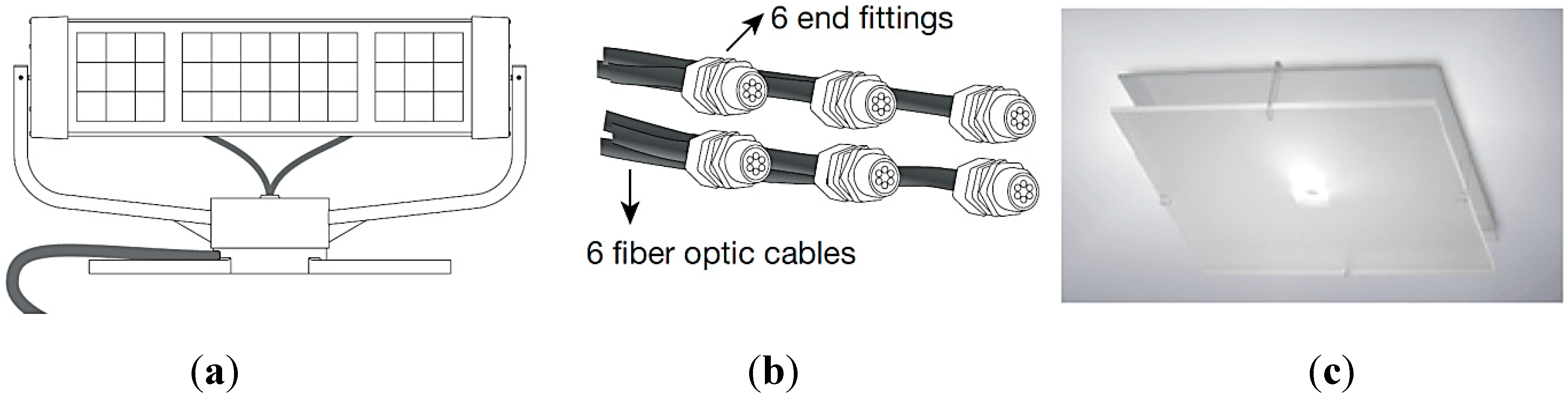
As an optical design, the receiver uses lenses to capture and concentrate the optimal amount of sunlight into the fiber optic cable to immediately transfer light inside a building. The properties of the receiver are as follows: 1140 mm × 570 mm × 270 mm dimensions, 32 kg weight, AC 100–240 V power supply, 50–60 Hz, 0–10 W power consumption, −20 °C to 40 °C operating temperature, and 5500 ± 300 lm light output. The receiver is made of aluminum, tempered glass, zinc/nickel steel, and acrylic materials.
- (ii)
Six solar fiber optic cables are attached together at a distance of 10 m from the receiver to a building interior. The selected cable length is 10 m based on the selection in previous research [
15,
22,
23]. The diameter of the fiber optic cable is 7 mm, with an end-fitting diameter of 18 mm. The fiber optic cable is made of acrylic, with a light transmission of 96.5%/m. The light output of each cable is 550 lm.
- (iii)
Six acrylic diffusers are connected to the end of the fiber optic cables. The 450 mm × 450 mm size of the six diffusers seems to be the most suitable based on the installation flexibility in configuring the position of the light diffusers to suit the research methodology and objective.
Figure 1.
(
a) Main components of the fiber optic daylighting system: receiver; (
b) fiber optic cables; (
c) and diffuser [
13].
Figure 1.
(
a) Main components of the fiber optic daylighting system: receiver; (
b) fiber optic cables; (
c) and diffuser [
13].
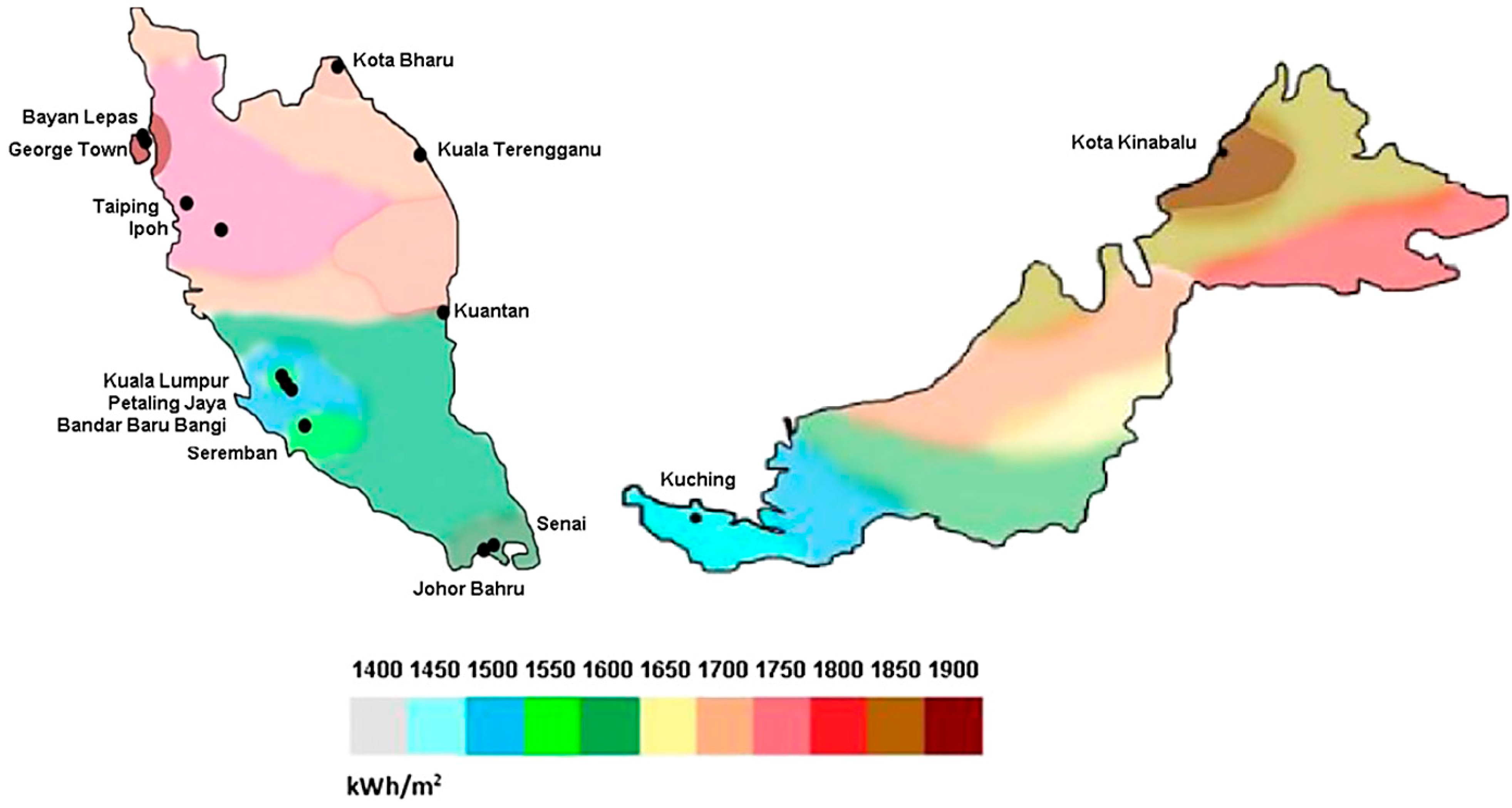
For experimental optimization, the selected location was at latitude 5°3ʹ N and longitude 100°3ʹ E in the School of Housing, Building, and Planning, Universiti Sains Malaysia, Penang, Malaysia. This location has a high solar radiation effect throughout the year, which ranges from 1750 to 1850 kWh/m
2/year, as shown in
Figure 2 [
24].
Figure 2.
Annual average solar insolation in Malaysia [
24].
Figure 2.
Annual average solar insolation in Malaysia [
24].
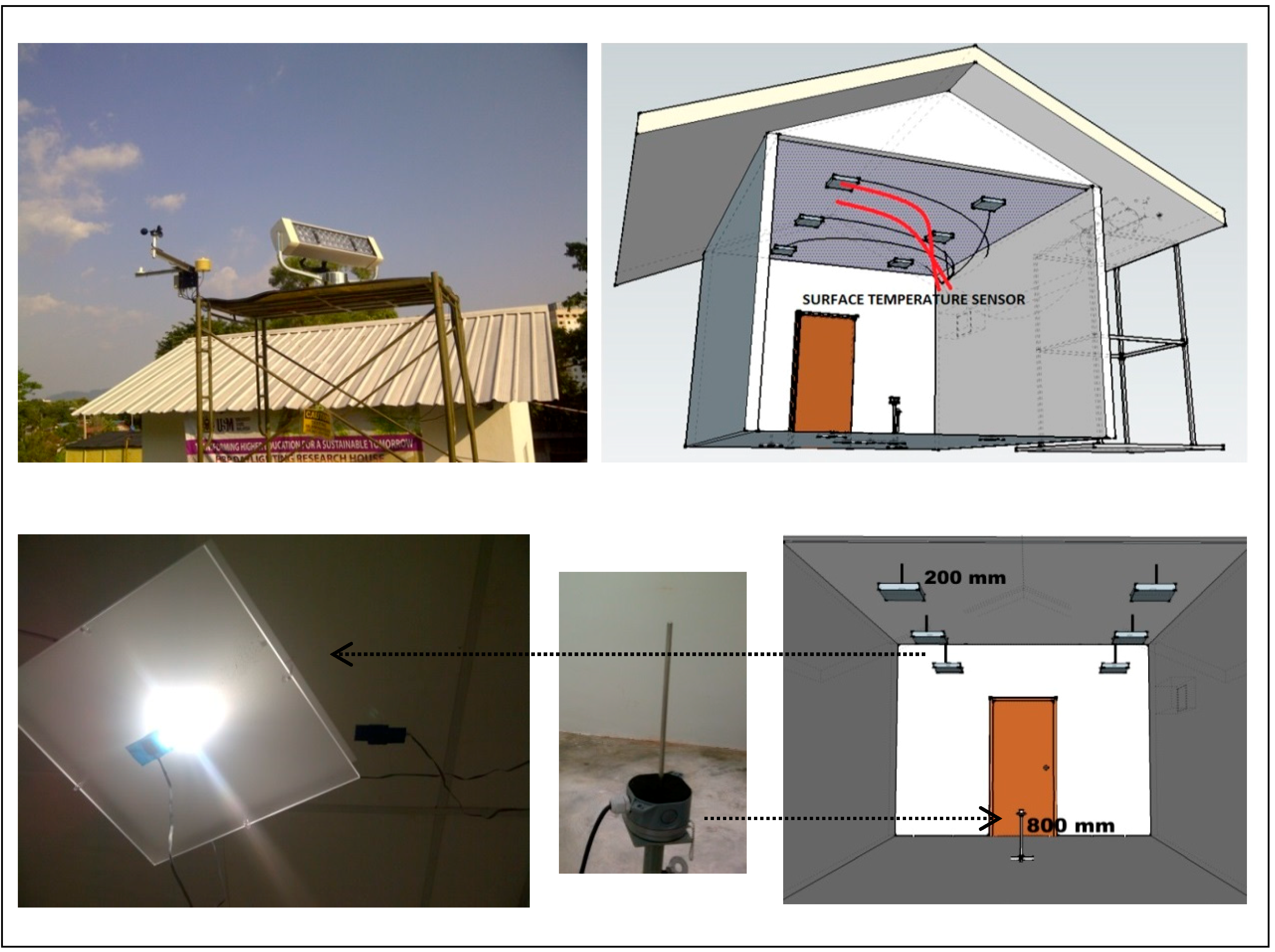
A typical standard working room was constructed with 5 m (L) × 4 m (W) × 3 m (H) dimensions and was used as the test bed. This test bed was built from normal clay brick and had double plastering for walls, normal cement rendering screed as floor finishes, and a set of gypsum boards as ceiling panels. These materials are standard construction materials in the Malaysian building industry, and thus, they provide realistic indoor climatic readings.
Various parameters were targeted to support the research objective. The parameters involved were outdoor and indoor air temperatures, internal surface temperature for lighting diffusers, and a ceiling board. A full-scale field study was performed based on local regulations, practices, the Malaysian tropical climate MS1525:2007 [
25] and the Green Building index [
26]. Data from the full-scale field study were collected through a computer program logged by the BABUC and Data Acquisition System that were connected to four newly calibrated sensors that logged every 5 min for a 17-day period starting from 22 May 2013 to 8 June 2013. Six days were presented for the analysis. Among which, three days (22 May, 28 May, and 1 June) were chosen when the system worked effectively at 80%–90%, whereas the remaining three days (5 June, 6 June and 8 June) were chosen when the system was off and nearly had the same outdoor conditions when the system was active. As shown in
Figure 3, the outdoor air temperature sensor was located at a level of approximately 3000 mm above the ground, whereas the indoor air temperature sensor was fixed at a level of 800 mm from the model floor. The diffusers were suspended at a level of 2800 m from the floor and 200 mm from the ceiling.
Figure 3.
Main tool sets (outdoor and indoor air temperatures: surface temperature at the diffusers and the ceiling) in the measurement model.
Figure 3.
Main tool sets (outdoor and indoor air temperatures: surface temperature at the diffusers and the ceiling) in the measurement model.
3. Results and Discussion
Data collected continuously for a 6-day period were analyzed between 08:00 and 18:00 because this period is the typical office working hours. Initially, the specified dates were evaluated thermally to identify the weather conditions when the system was on and off.
Figure 4 shows the conditions of the targeted days, which are assessed through comparative evaluation to eliminate uncertainties on the effect of outdoor conditions on the performance of the fiber optic daylighting system.
The results in
Figure 4 show that during the six-day period, nearly the same conditions were experienced, which were recorded every day starting from approximately 27 to 28 °C, while the maximum temperature reached was approximately 36 °C. The ending result was approximately 32 °C, except on 6 May, which was the only day when the reading stopped at 34.6 °C. Given that the model was constructed in an actual environment, obtaining similar weather conditions was difficult. However, the results presented similar weather patterns on the selected days.
Figure 4.
Comparative outdoor air temperature data when the system was on and off.
Figure 4.
Comparative outdoor air temperature data when the system was on and off.
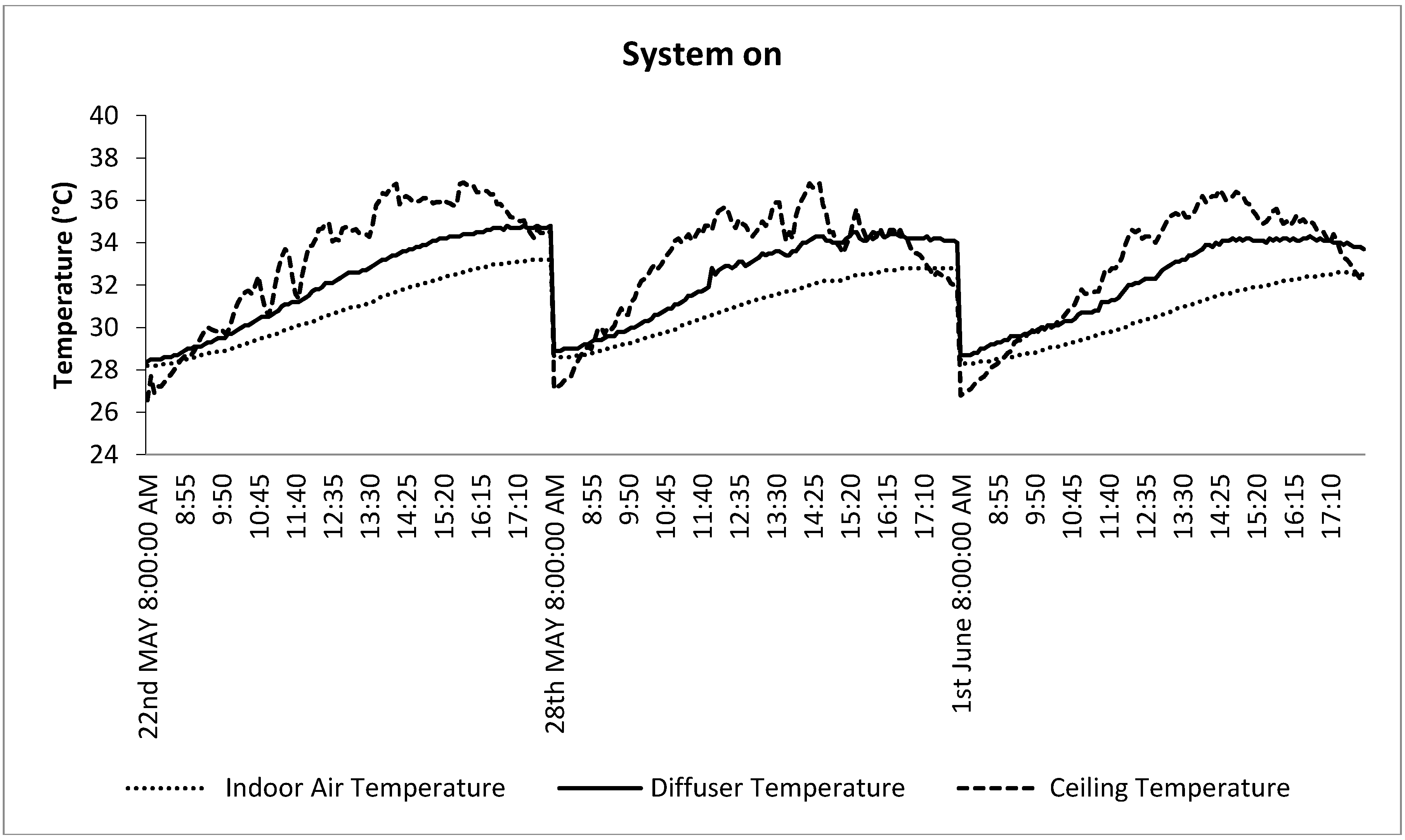
Moreover, the indoor environment exhibited a different behavior.
Figure 5 shows the indoor environment when the system is on. The results of the comparative evaluation indicate that the diffuser surface temperature (DST) of the fiber optics performed moderately between indoor air temperature (IAT) and ceiling surface temperature (CST).
DST and IAT exhibited similar performance patterns on the first day (22 May), when the readings started to be higher in the morning with 0.3 °C (28.5 °C DST–28.2 °C IAT), hit a maximum at 15:15 with 1.9 °C (34.2 °C DST–32.3 °C IAT), and stopped with a difference of 1.6 °C (34.8 °C DST–33.2 °C IAT). On 28 May, the readings started to be higher in the morning with 0.3 °C (28.9 °C DST–28.6 °C IAT), hit a maximum from 14:25 to 14:35 with 2.2 °C (34.2 °C DST–32 °C IAT), and stopped with a difference of 1.3 °C (34.1 °C DST–32.8 °C IAT). On 1 June, the readings started to be higher in the morning with 0.4 °C (28.7 °C DST–28.3 °C IAT), hit a maximum from 14:05 to 14:45 with 2.6 °C (33.9 °C DST–31.3 °C IAT), and stopped with a difference of 1.3 °C (33.8 °C DST–32.5 °C IAT).
However, the relationship between DST and the CST exhibited dissimilar patterns. The readings for DST presented a linear progression, whereas those for CST exhibited an irregular progression because the ceiling condition was directly affected by outdoor weather conditions. In general, ceiling temperature is always less than that of the diffusers during the starting time in the morning and at the ending time of the day. However, temperature was irregular during peak time, during which the maximum difference recorded on 22 May at 14:10 was 3.4 °C (36.8 °C CST–33.4 °C DST), on 28 May at 11:05 was 3.1 °C (34.2 °C CST–31.1 °C DST), and on 1 June at 14:25 was 2.6 °C (36.5 °C CST–33.9 °C DST).
Figure 5.
Performance of the indoor air temperature, diffuser temperature, and ceiling temperature when the system is active.
Figure 5.
Performance of the indoor air temperature, diffuser temperature, and ceiling temperature when the system is active.
Based on the aforementioned readings, the differences in behavior between DST and IAT at the starting point were approximately 0.3, 0.3 and 0.4 °C; reached the maximum of approximately 1.9, 2.2 and 2.6 °C; and nearly stabilized at 1.6, 1.3 and 1.3 °C at the ending point. However, the maximum differences between DST and CST were 3.4, 3.1 and 2.6 °C.
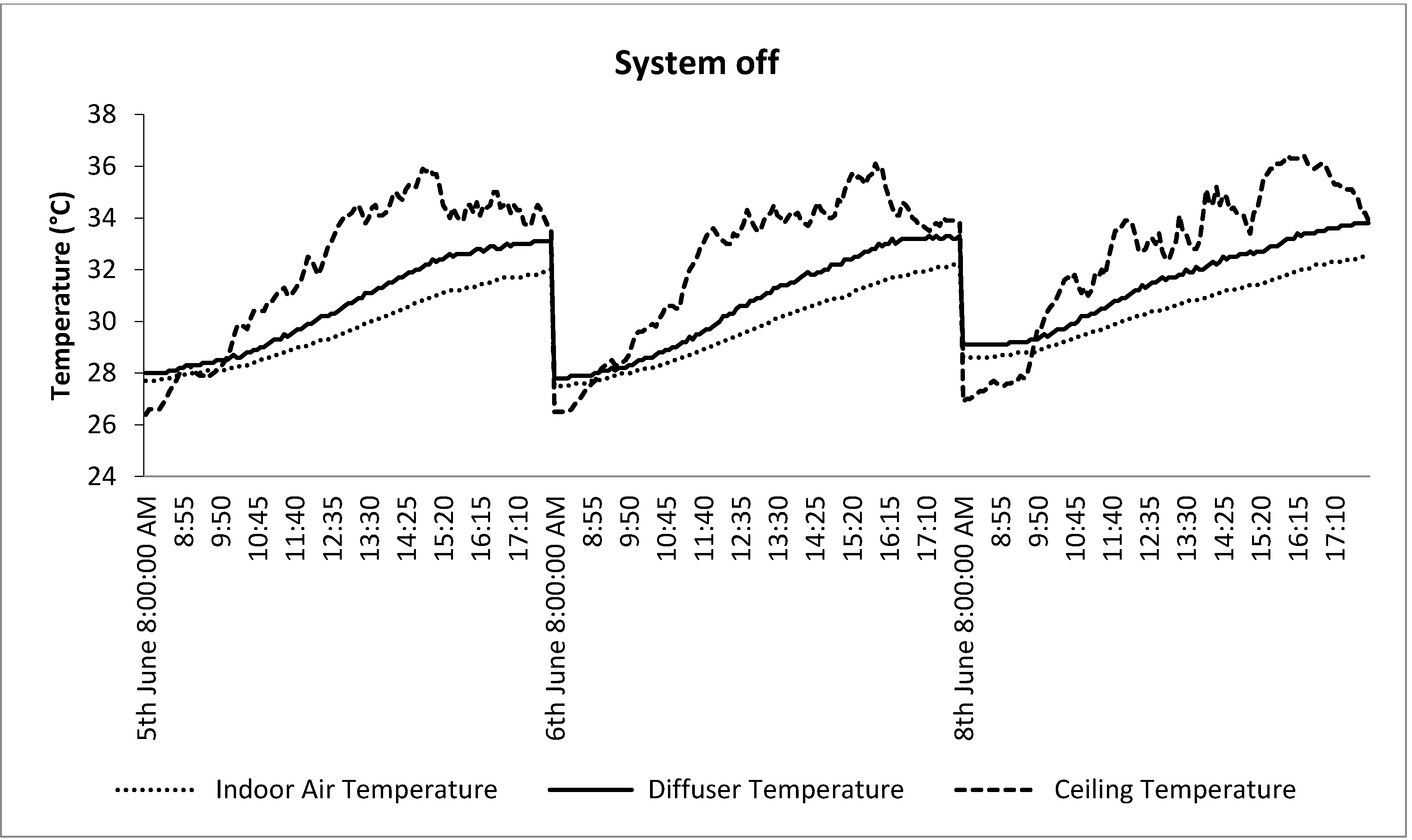
Moreover, the effect of the fiber optic daylighting system when the system was inactive clearly indicates a huge difference, as shown in
Figure 6. The results of the comparative evaluation indicate that DST performed moderately between IAT and CST, but had a lower value that was close to IAT. These findings clearly indicate a heat reduction in the fiber optic diffuser compared with the results when the system was active (
Figure 5).
DST exhibited a similar pattern as IAT, with a difference on the first day (5 June) when the readings started to be higher in the morning with 0.3 °C (28 °C DST–27.7 °C IAT), hit a maximum from 15:25 to 16:10 with approximately 1.4 °C (32.8 °C DST–31.4 °C IAT), and then stopped with a difference of 1.1 °C (33.1 °C DST–32 °C IAT). On 6 June, the readings started to be higher in the morning with 0.3 °C (27.8 °C DST–27.5 °C IAT), hit the maximum at 16:00 with 1.5 °C (33 °C DST–31.5 °C IAT), and then stopped with a difference of 1.1 °C (33.3 °C DST–32.2 °C IAT). On 8 June, the readings started to be higher in the morning with 0.5 °C (29.1 °C DST–28.6 °C IAT), hit the maximum at 16:15 with 1.5 °C (33.4 °C DST–31.9 °C IAT), and then stopped with a difference of 1.3 °C (33.8 °C DST–32.5 °C IAT).
The relation between DST and CST were also incompatible because ceiling conditions were affected directly by outdoor weather conditions. In contrast to the first condition, CST was generally always less than that of DST during the starting time in the morning and continued to remain higher even when the temperature dropped at the ending time of the day. This finding also supports the results that fiber optic cables generate heat when the system was active. However, the relation between the ceiling and the diffuser showed that the temperature of the former was always higher and rose in the same direction even in unsteady conditions. The uneasy relationship between the two temperatures during the peak time recorded a maximum difference on 5 June at 14:50 with 3.8 °C (35.9 °C CST–32.1 °C DST), on 6 June from 11:50 to 11:55 with 3.8 °C (33.5 °C CST–29.7 °C DST), and on 8 June from 15:45 to 16:00 with 3.2 °C (36.4 °C CST–33.2 °C DST).
Figure 6.
Performance of the indoor, diffuser, and ceiling temperatures when the system was inactive.
Figure 6.
Performance of the indoor, diffuser, and ceiling temperatures when the system was inactive.
According to the preceding evaluations, the differences between DST and IAT recorded at the starting point were 0.3, 0.3 and 0.5 °C; reached a maximum at approximately 1.4, 1.5 and 1.5 °C; and nearly stabilized at 1.1, 1.1 and 1.3 °C at the ending point. However, the maximum differences between DST and CST were 3.8, 3.8 and 3.2 °C.
Based on
Figure 7, the DSTs in the two cases were clearly different. In the first condition, the readings showed that DST was always at a higher level on 22 May with 34.8 °C from 17:20 to 18:00, on 28 May with 34.5 °C from 15:30 to 16:00, and on 1 June with 34.3 °C at 16:40. The variations of peak time were caused by the duration of the system while working constantly without stopping. However, when the system was off, the readings for DST showed that the maximum temperature was 33.1 °C from 17:35 to 18:00 on 5 June, 33.3 °C from 17:15 to 18:00 on 6 June, and 33.8 °C from 17:40 to 18:00 on 8 June.
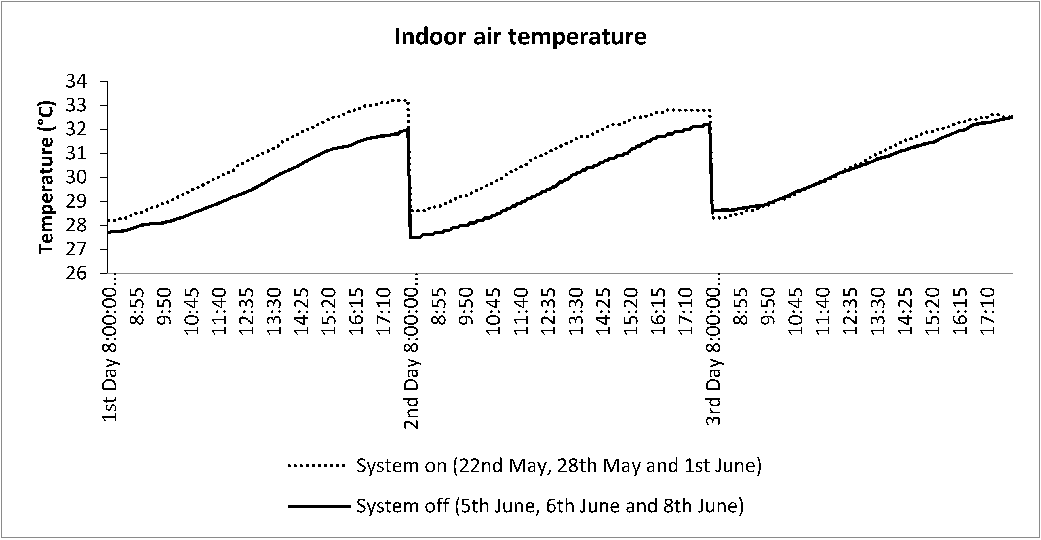
However, the readings in
Figure 8 also proved that indoor temperature dramatically affected indoor environmental conditions when the system was active. The results when the system was active indicate that the maximum temperature was 33.2 °C from 17:25 to 18:00 on 22 May, 32.8 °C from 16:35 to 18:00 on 28 May, and 32.6 °C from 17:20 to 17:30 on 1 June. However, the readings showed that when the system was off, the maximum temperature was 32 °C from 17:55 to 18:00 on 5 June, 32.2 °C from 17:50 to 18:00 on 6 June, and 32.5 °C from 17:50 to 18:00 on 8 June. The readings on 8 June when the system was off exhibited irregularities that were near the conditions when the system was on because the effect of the outside conditions was the greatest on this date (
Figure 4).
Figure 7.
Performance of DST when the system was on and off.
Figure 7.
Performance of DST when the system was on and off.
Figure 8.
Performance of IAT when the system was on and off.
Figure 8.
Performance of IAT when the system was on and off.
Given that these results have realized the actual aim of the study, the researchers doubted the effects of CST and IAT on the thermal behavior of the diffuser.
Figure 9 and
Figure 10 show the relation of DST with IAT and CST. In general, the readings in
Figure 9 indicate that the difference between DST and CST was lower when the system was active and higher when the system was off. The readings showed that the two conditions nearly had the same difference during that period, particularly at approximately 14:00, in terms of the effect of external weather conditions.
Figure 9.
Relationship of the difference between DST and CST when the system was on and off.
Figure 9.
Relationship of the difference between DST and CST when the system was on and off.
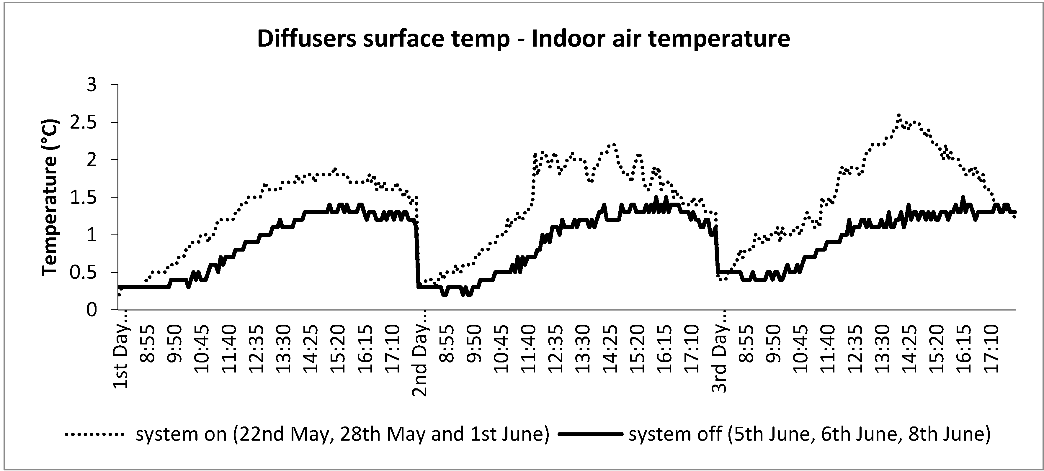
In addition,
Figure 10 also indicates the significant effect of heat from the end point of the fiber optic cables when the system was on. This figure also shows the difference between DST and IAT when the system was active and inactive. The readings imply the presence of heat generated from the fiber optic cables. They showed that the peak difference was 1.9 °C at 15:15 on 22 May, 2.2 °C from 14:25 to 14:35 on 28 May, and 2.5 °C from 14:05 to 14:45 on 1 June. However, the results showed that when the system was off, the peak difference was 1.4 °C from 15:25 to 16:10 on 5 June, 1.5 °C at 16:00 on 6 June, and 1.5 °C at 16:15 on 8 June. The difference between the two conditions showed an increase in heat gain ranging from 0.5 °C to 1 °C.
Figure 10.
Relationship of the difference between DST and IAT when the system was on and off.
Figure 10.
Relationship of the difference between DST and IAT when the system was on and off.
Therefore, the results of the analysis tests indicate that the Parans SP3 system generates heat under the Malaysian climate, which directly affects the behavior of indoor conditions.
Table 1 and
Table 2 provide a summary of the findings obtained from this investigation.
Table 1.
Total results of DST and IAT when the system was on and off.
Table 1.
Total results of DST and IAT when the system was on and off.
| Date | Diffuser Surface Temperature (°C) | Indoor Air Temperature (°C) |
|---|
| Max | Average | Min | Max | Average | Min |
|---|
| System On | | |
| 22 May | 34.8 | 32.1 | 28.4 | 33.2 | 30.8 | 28.2 |
| 28 May | 34.5 | 32.4 | 28.9 | 32.8 | 31 | 28.6 |
| 1 June | 34.3 | 32.1 | 28.7 | 32.6 | 30.6 | 28.3 |
| System Off | | |
| 5 June | 33.1 | 30.6 | 28 | 32 | 29.7 | 27.7 |
| 6 June | 33.3 | 30.7 | 27.8 | 32.2 | 29.8 | 27.5 |
| 8 June | 33.8 | 31.4 | 29.1 | 32.5 | 30.5 | 28.6 |
Table 2.
Average three-day readings of DST and IAT when the system was on and off.
Table 2.
Average three-day readings of DST and IAT when the system was on and off.
| Item | Diffuser Surface Temperature (°C) | Indoor Air Temperature (°C) |
|---|
| Max | Average | Min | Max | Average | Min |
|---|
| System On | 34.5 | 32.2 | 28.6 | 32.8 | 30.8 | 28.3 |
| System Off | 33.4 | 30.9 | 28.3 | 32.2 | 30 | 27.9 |


