1. Introduction
As reported in the IPCC 5th Assessment Report (IPCC AR5) [
1], the impact of climate change will continue to be associated with monetary and non-market costs across the globe. The recognized impact of emissions of greenhouse gases and trends in energy consumption in cities has drawn attention in past decades in the literature. Cities are the hearts of economic activity, and nearly half of the world’s population lives in cities. Therefore, growing city-related issues have become the centers of policy discussions in terms of governance [
2]. The importance of adopting proper design and implementing responses at the city or regional level is increasingly recognized as crucial to adaptation and mitigation action (C40 Large Cities Climate Leadership Group). The main purpose of this study is to investigate the relationships between population trends, historical energy consumptions, the changes of average electricity price, annual average temperature, and extreme weather events for three selected cities: New York, Chicago, and Los Angeles.
Effective management of various factors (such as the energy consumptions, the emission of greenhouse gases, and land use changes,
etc.), significantly reducing the rate of climate change, is often referred to as mitigation. Climate and weather events may be differentiated by their wide range of spatial, temporal, and geographic contexts [
3,
4]. According to the World Meteorological Organization, “At the simplest level the weather is what is happening to the atmosphere at any given time. Climate in a narrow sense is usually defined as the “average weather”, or more rigorously, as the statistical description in terms of the mean and variability of relevant quantities over a period of time” [
5]. For example, a heat wave in Chicago and Paris, based on a lengthy duration of a specified threshold temperature [
6], could be similar to a season of average temperatures in Dubai’s climatological day records. An unusual two-week snowstorm in the southeastern U.S. that cancelled schools could be experienced as normal in, say, Alaska during that state’s winter season. Thus, cities differ at least economically, demographically and climatically, and as a result, each will have different energy needs and require different mitigation strategies regarding energy use.
2. Background
Studies show that the potential impact of climate change on states and cities depends on a variety of social, economic, and environmental determinants. For example, flood events and heat waves may cause more severe impacts and induce a relatively higher level of vulnerability in cities that have high population density, intensively used urban drainage systems, and urban-specific underground transport systems [
7]. Many cities (such as New York, Los Angeles, Chicago, and Boston) rely on imported food items from surrounding rural areas and/or other countries. The impact of climate change and extreme events on agricultural production and food distribution certainly influences the economy and quality of life in affected cities [
8].
Potential impact and consensus findings on climate change and/or extreme events in cities have drawn attention in the literature. The variety of types of impact include the effects of extreme events (e.g., floods, heat waves, droughts, floods, and storms) on infrastructure, energy usage (e.g., water, cooling, and heating), sea level rise (on coastal cities), resources, and health (e.g., extreme events
vs. mortality, vector-borne diseases) [
9,
10,
11,
12,
13]. Other direct, indirect, and/or induced effects of climate change and/or extreme events include those on air pollution, tourism, and urban biodiversity [
14,
15,
16].
2.1. The Impact of Climate Change on Cities/States
Notable studies undertaken to date are both quantitative and qualitative, focused on analyses of city-scale impacts in terms of physical and/or monetary effects and strategic management that are relevant to climate change assessments’ mitigation and adaptation options. Examples of cities studied include Boston, New York, London [
17,
18,
19,
20,
21,
22,
23,
24], cities in Canada (e.g., Toronto, Montreal, Vancouver) [
25], cities in Australia and New Zealand (e.g., Sydney, Melbourne, Wellington) [
26,
27], and cities in Asia [
28]. However, across these reported city-scale studies, there has been more of a focus on coastal cities and less information pertaining to inland cities’ issues such as changes in population trends, energy demand, river flooding, and quality of water resources [
29]. Additionally, many quantitative measurements employed across geographical locations of studied cities demonstrate a gap in consistency in terms of impact scenarios and evaluations of monetary assessments for market and non-market effects.
Because of the constraints of physical infrastructure capacity, increased density of population, and existing deficits of adaptation and mitigation, cities in developing countries are likely to have relatively higher vulnerabilities than those in the developed world. Several previous studies have investigated various impacts of climate change on cities, such as using impact assessments related to policy-making regarding climate change adaptation. Across continents, in order to obtain benefits of maximizing incorporated aids in raising knowledge and implementing solutions for the impact of climate change on communities, noted megacities have aimed to establish initiatives that can transfer research methods and proper adaptation strategies collaboratively to cities that show similar vulnerability characteristics. Sea level rise and the impact of extreme storms on coastal cities are the most studied topics over the past two decades. The effectiveness of energy consumption in cities is likewise one of the most prioritized topics for study.
2.2. The Demands of Energy Consumption
The demands of energy consumption have been identified as a key factor that affects an economy at the city, national, and international level. Studies project an increasing cooling demand in summer seasons in the south and an increasing heating demand in winter in the north [
30]. Winter heating energy demands are associated with fossil fuels, while summer cooling energy demands mainly rely on electricity. In urban cities, air conditioning usage is expected to increase because of the density of residential and business populations, concentration of business flow, and possible urban heat island effects.
According to IPCC AR5 [
31], in tropical and subtropical cities, space cooling takes up a significant amount of electricity. For example, Hong Kong’s and Riyadh’s business sectors’ air conditioning accounts for nearly 60% of total electricity use. Miller
et al. [
32] note that residential and commercial air conditioning in summer comprised 30% of total electricity use in California in the past decade. Building design, advanced air conditioning models, energy efficiency installations, solar panel roofs, and any other uncertainties may impact the overall energy efficiency of buildings in cities [
33,
34].
2.3. Effects of Extreme Hot and Cold Events
There are discussions of increase in heat-related mortality and reduction in cold-related mortality because of the likelihood of climate change’s impact on temperature variations [
35]. Heat waves and extreme drought events have also had various impacts in cities and regions [
36]. Gosling
et al. [
37] listed the methodology comparisons and overviewed the limits and merits of utilizing quantitative
vs. qualitative approaches in terms of health effects of extreme hot and cold events. The studied cities included Boston [
24], New York [
38], Los Angeles [
39], cities in Australia and New Zealand [
40,
41], cities in the Eastern U.S. [
42], cities in the Midwestern U.S. [
43], and Lisbon [
44] that predicted the average mortality rate might decrease if proper adaptation, such as storm and heat alert systems and awareness of impacts of extreme events, could be implemented effectively. Although there are statistically higher population densities and disease transmission rates in developing countries, the relationships between population exposure, cities’ vulnerability, and level of mutuality in extreme storm/heat alert systems may be further investigated across underdeveloped, developing, and developed regions. Data on the costs and benefits of controlling and monitoring the number of deaths caused by climate-related diseases and extremes also need to be systematically established and integrated in public health systems and risk prevention approaches [
45,
46].
Comprehensive strategic plans are needed on the part of government policy, industries, and environmental activists. Economists and politicians have argued about the costs and benefits regarding transportation fuels’ transitions. Indeed, minimizing the level of ethanol in gasoline may reduce greenhouse gas emissions, according to Congress’s Renewable Fuel Standards (RFS). However, some have argued that the RFS would have a positive impact on the transportation fuels transition, while some predicted the cost of implementing the ethanol policy would generate higher costs [
47].
According to the ‘All-of-the-above energy strategy’ introduced by the President’s Climate Action Plan [
48], America aims to advance its energy independence, supply affordable cleaner energy that will induce economic growth, and generate employment opportunities for a clean-energy economy. Specifically, the U.S. government wants to reduce pollution to improve public health; lead the county to become independent from foreign oil as the country is now at a 40-year low in terms of dependence on foreign oil; and advance clean energy deployment continuously [
48].
3. The Purpose of the Study
Contributions to total U.S. greenhouse gas emissions in 2012 by various economic sectors included electricity (31%), transportation (28%), industry (20%), agriculture (10%), and commercial and residential (10%) [
48]. The main purpose of this study is to investigate the relationships between population trends, historical energy consumptions, the changes of average electricity price, annual average temperature, and extreme weather events for three selected cities: New York, Chicago, and Los Angeles. These cities were selected because they represent three main metropolitan cities in the East, Middle, and the Western regions of the U.S., with well-rounded industrialization along with vital economic growth roles. The three cities (states) have encountered various issues over the years, and represent some of the most vulnerable locations to the adverse effects of climate change. New York City (New York) was hit by Hurricane Sandy, Chicago (Illinois) experienced heat stress with (most notably) the 1995 heat wave, and Los Angeles (California) continues to be threatened by wild fires. All three cities reported high annual growth or frustration rates in their various industrial sectors (e.g., manufacturing) impacted by macro/micro factors (e.g., unemployment rate) due to these extreme events. Yet the heavy demands of energy consumption that lead to climate change and a consequent increase the frequency and intensity of these events in cities are important for maintaining and sustaining sufficient economic growth. Our study investigates the relative significance of three contributors to energy use in cities as a first step towards the development of policy-relevant mitigation strategies.
4. Methods
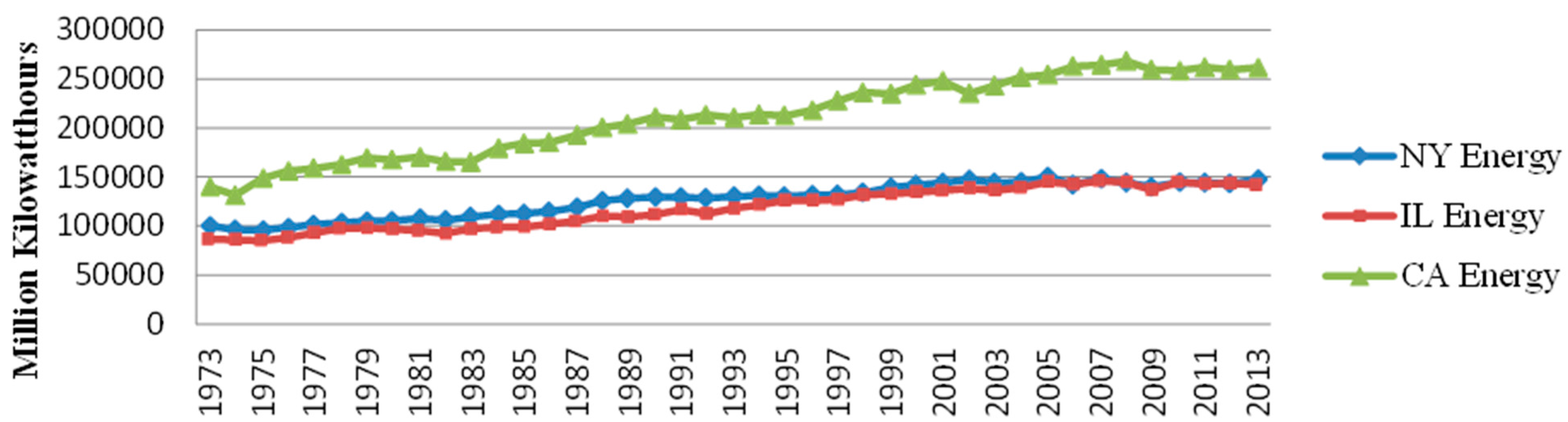
In order to investigate the relationships between variables, such as the causal effect of one variable upon another, regression analysis is a commonly adopted statistical tool. In the field of econometrics, regression techniques have been employed to estimate how a key variable is impacted by the quantitative effects of a list of identified causal/independent variables. In this study, total energy consumption data sets (
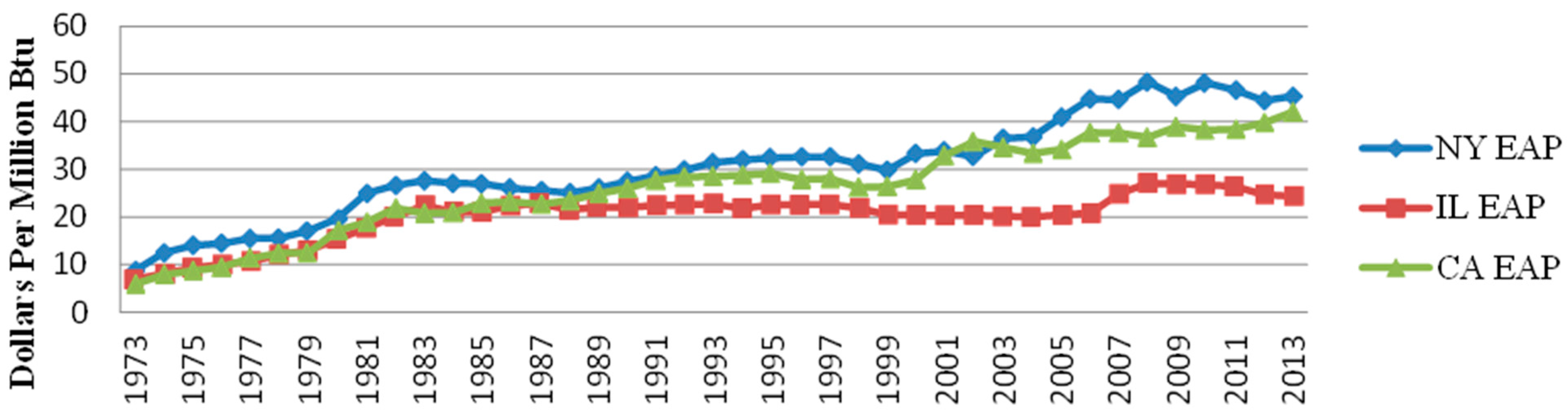
Figure 1) and the average electricity price list (
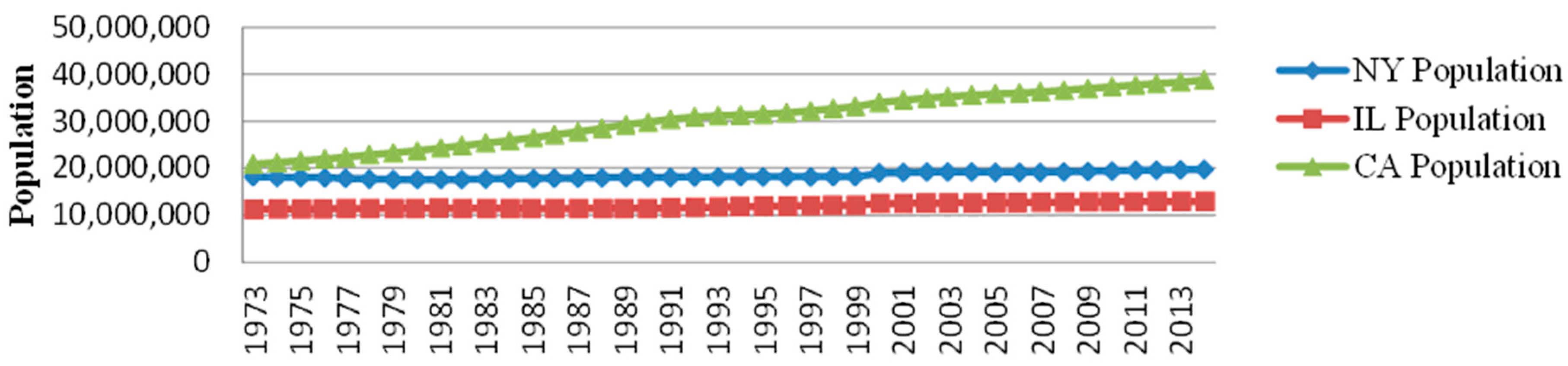
Figure 2) were provided by the U.S. Energy Information Administration. Population data sets (
Figure 3) were provided by the U.S. Census Service, the monthly and annual temperature data sets (
Figure 4), and heat waves data sets are retrieved from the National Climatic Data Center.
Figure 1.
Energy total consumption (1973–2013).
Figure 1.
Energy total consumption (1973–2013).
Figure 2.
Electricity average price (EAP) (1973–2013).
Figure 2.
Electricity average price (EAP) (1973–2013).
Figure 3.
Population trends (1973–2013).
Figure 3.
Population trends (1973–2013).
Figure 4.
Average temperature (AT) (1973–2013).
Figure 4.
Average temperature (AT) (1973–2013).
Total energy consumptions (TEC) are affected by a variety of factors such as changes of population and electricity average price (EAP), factors that were aggregated into the noise term in the regression model. A multiple regression model permits multiple factors to be included within the model in order to estimate the effects of each of the impact factors on the dependent variable. Because a simple regression model may produce omitted variables bias, a multiple regression model is more suitable for the purposes of this study. We employed three independent variables within the total energy consumption analysis; population, electricity average price, and average county temperature. Holding constant the level of population, we expect the higher electricity average price would induce lower energy consumption (due to consumers’ efforts to economize.) Let EAP denote annual electricity average prices in the energy business field and, as in the case of population, we assumed that it has a linear effect upon total energy consumption that is stable across the studied three states. The first multiple regression model may be written as follows:
where
TEC = total energy consumption;
α is the intercept, the model-predicted value of the dependent variable when the value of every predictor is equal to 0.
P is the population predictor of total energy consumption
B is the coefficient value of the population,
EAP is the electricity average price predictor of total energy consumption,
γ is the coefficient value of the electricity average price (EAP), and
ε is the error in the observed value.
The Multiple regression model investigates a range of explanatory variables. With the total energy consumption (TEC)-axis [where population (P) and electricity average price (EAP) are zero] implies a constant term α, its slope in the population dimension implies the coefficient β, and its slope in the electricity average price dimension implies the coefficient γ. Specifically, in the model TEC = α + βP + γEAP + ε, α captures total energy consumption without the effects of population or electricity average price. β is an estimate of the effect of population on total energy consumption, holding Electricity Average Price constant. γ is the estimated effect of electricity average price on total energy consumption, holding population constant.
Multiple regression analysis uses a minimum of the sum of squared errors, which is the vertical distance between the actual value of total energy consumption and the tested and identified explanatory variables, to determine the fit of the equation to the data. Using the observed values of the dependent and independent variables, through the statistical properties of regression, the values of α, β, γ and the noise term ε were estimated. When there are n explanatory variables within the multiple regression analysis, the estimation procedure will ensure that the sum of squared errors is minimized. The constant term represents the intercept and every coefficient of every explanatory variable represents the slopes for the variables within the equation. The goal of the regression is to minimize the sum of square errors (SSE), an estimator that depends upon the value of the error term, ε, drawn from the probability distribution of each parameter in the data set. When the mean of the probability distribution is equivalent to the true value of the estimated parameters, within the statistical procedure, the estimator can be taken to be unbiased.
The SSE criterion generates estimates that are consistent and unbiased when the noise term, ε, is drawn from a distribution of each listed observation that has a mean of zero. On the other hand, when the drawn noise terms of distributions from each listed observation have the same variance and are statistically independent of each other, the SSE indicates the most efficient estimates that indicate a linear function among the parameters.
Based on the identified data sets in this study, extremely hot summer months should stimulate higher energy consumption due to heavy uses of air conditioning while extremely cold winter months may induce higher energy consumption because of the extensive heat energy use. “Average temperature” is the annual average temperature of each studied city as recorded by observation weather stations. “Extreme” is a dummy variable that equals 1 for extreme temperature years (heat waves) and zero for regular average temperature that is within the normal ranges during the intermediate seasons for each year. Three key parameters of heat waves at an annual basis include intensity, duration, and frequency. The highest three continuous nighttime minima is defined as heat wave intensity (°C) [
6]. “
Heat wave duration (number of days during a heat wave) and frequency (number of heat wave events per year) are based upon two thresholds, T1 and T2, of daily maximum temperature. ... a heat wave as the longest continuous period satisfying three criteria: (a) the maximum daily temperature remained T1 or higher for at least three continuous days, (b) the mean daily maximum temperature is higher or equal to T1, and (c) in each day, the daily maximum temperature is no lower than T2” (p. 4) [
49]. In this study, we use T1 (the 97.5th) and T2 (81st percentiles) of daily maximum temperature (1973–2013) to define a heatwave event.
The independent variables are used to generate the “actual value” of total energy consumption for each of the 41 observations (1973–2013). We assume that there is a multiple linear relationship between the total energy consumption (the dependent variable) and selected predictors (population, electricity average price, average temperature, and heatwave events). The final proposed multiple regression formula is denoted as:
where
Y = total energy consumption;
Yj is the value of the jth case of the dependent scale variable,
i = 1,
j =
jth case
P is the population predictor of total energy consumption
B1ij is the coefficient value of the population
EAP is the electricity average price predictor of total energy consumption
B2ij is the coefficient value of the electricity average price (EAP)
AT is the average temperature predictor of total energy consumption
B3ij is the coefficient value of the average temperature,
Extreme is dummy variable:
B4ij is the coefficient value of the extreme weather event
P, EAP, AT, and Extreme are the predictors of Y
ε is the error in the observed value
b0 is the intercept, the model-predicted value of the dependent variable when the value of every predictor is equal to 0.
5. Results
During the selection procedure, we used a backward elimination approach that included all predictor variables included in the equation and then we sequentially removed the variable that has the smallest partial correlation with the dependent variable. When the first variable meets the elimination criteria, it is removed. A tolerance criterion was applied. A variable was not entered when it caused another existing variable in the model to drop its tolerance criterion (below 0.0001). For the remaining predictor variables, the same procedure is repeated until there are no more variables that meet the removal criteria. Within the linear regression model, the coefficient value is used to determine an increased value of the jth predictor by 1 unit at which point the value of dependent variable increases by bj units.
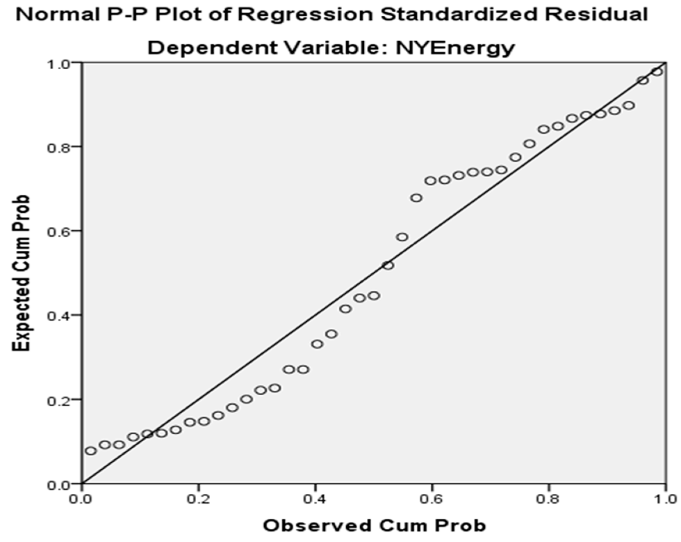
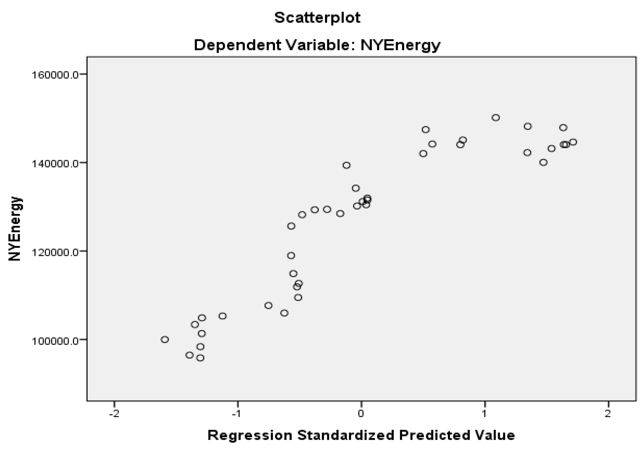
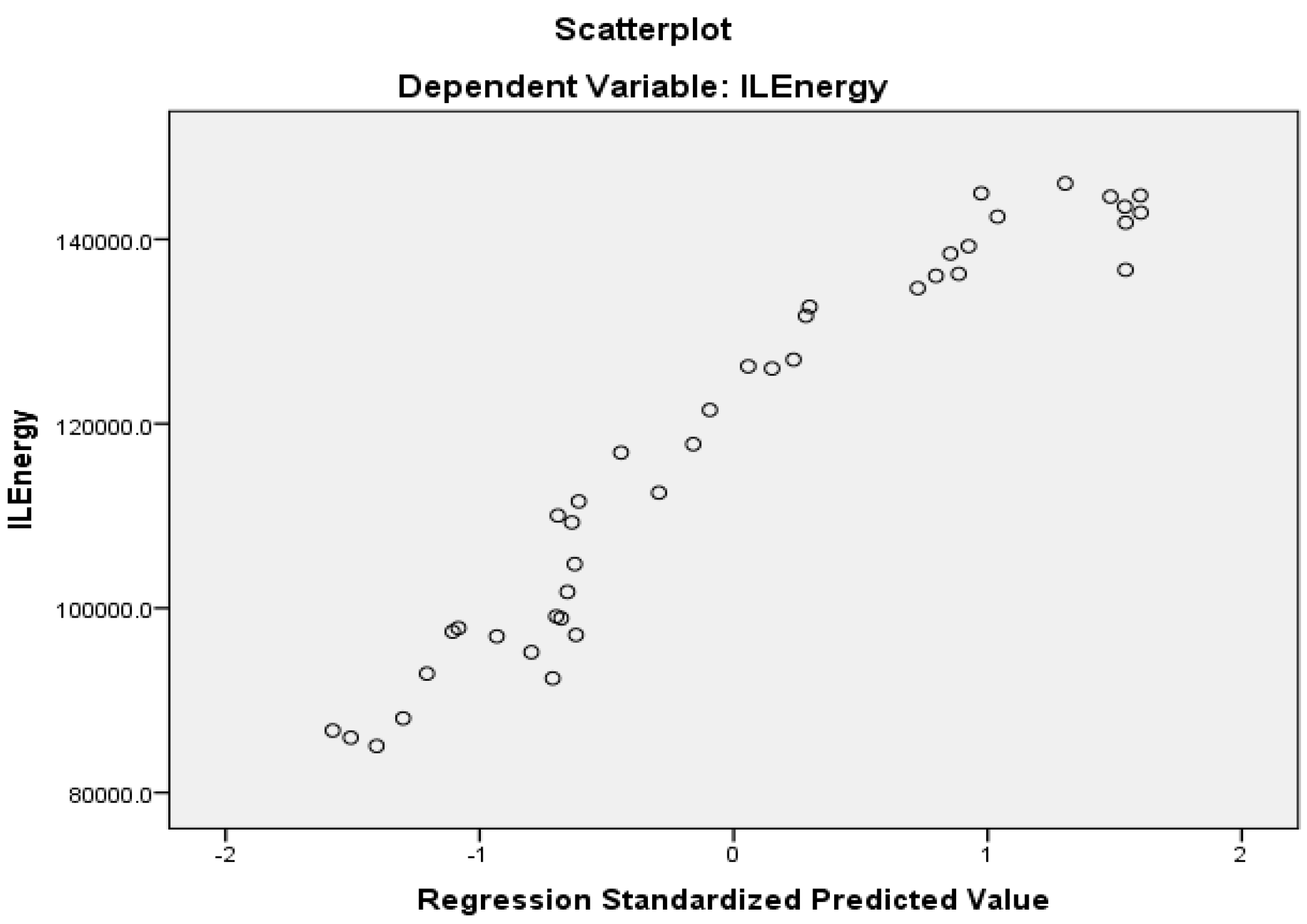
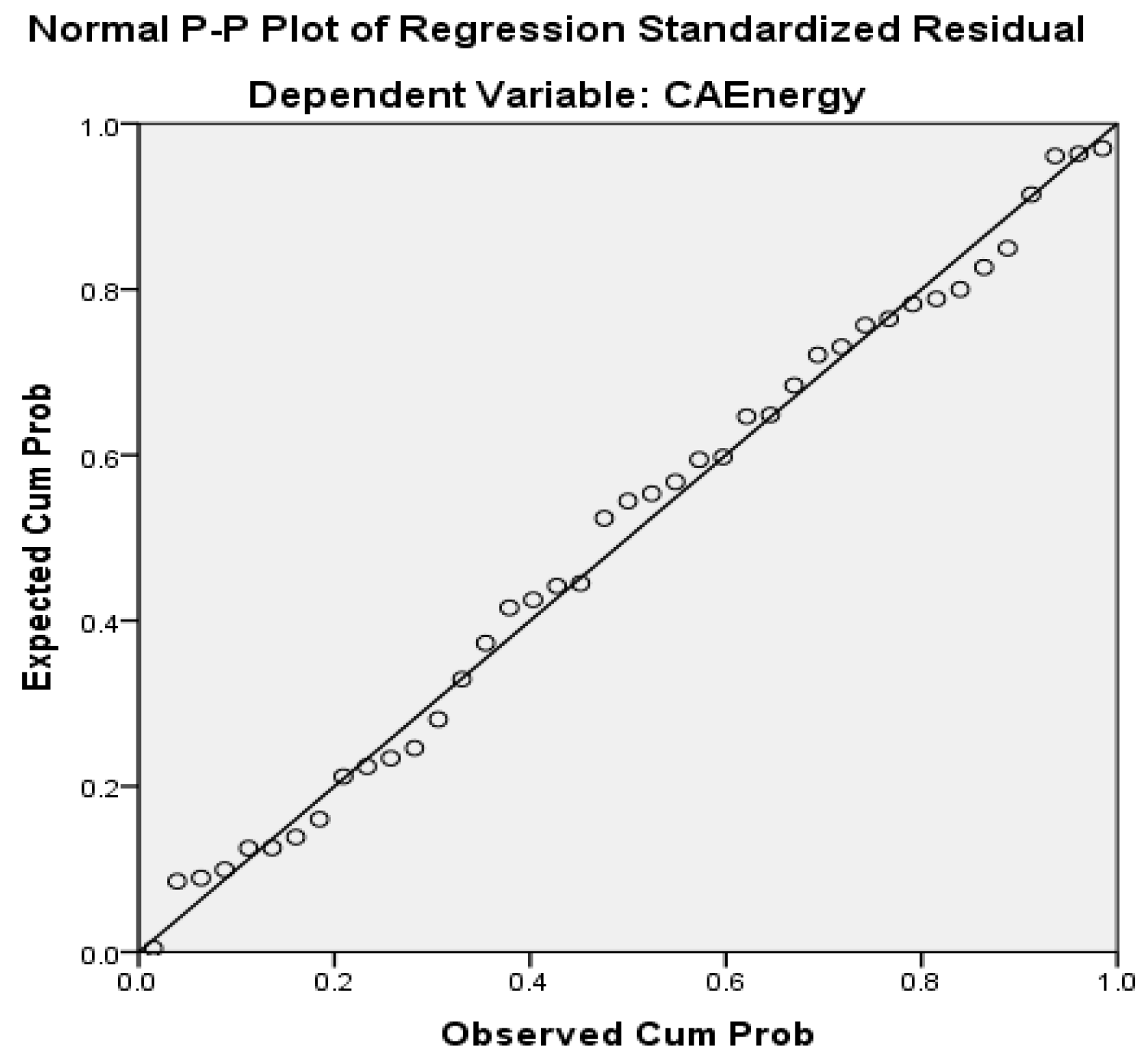
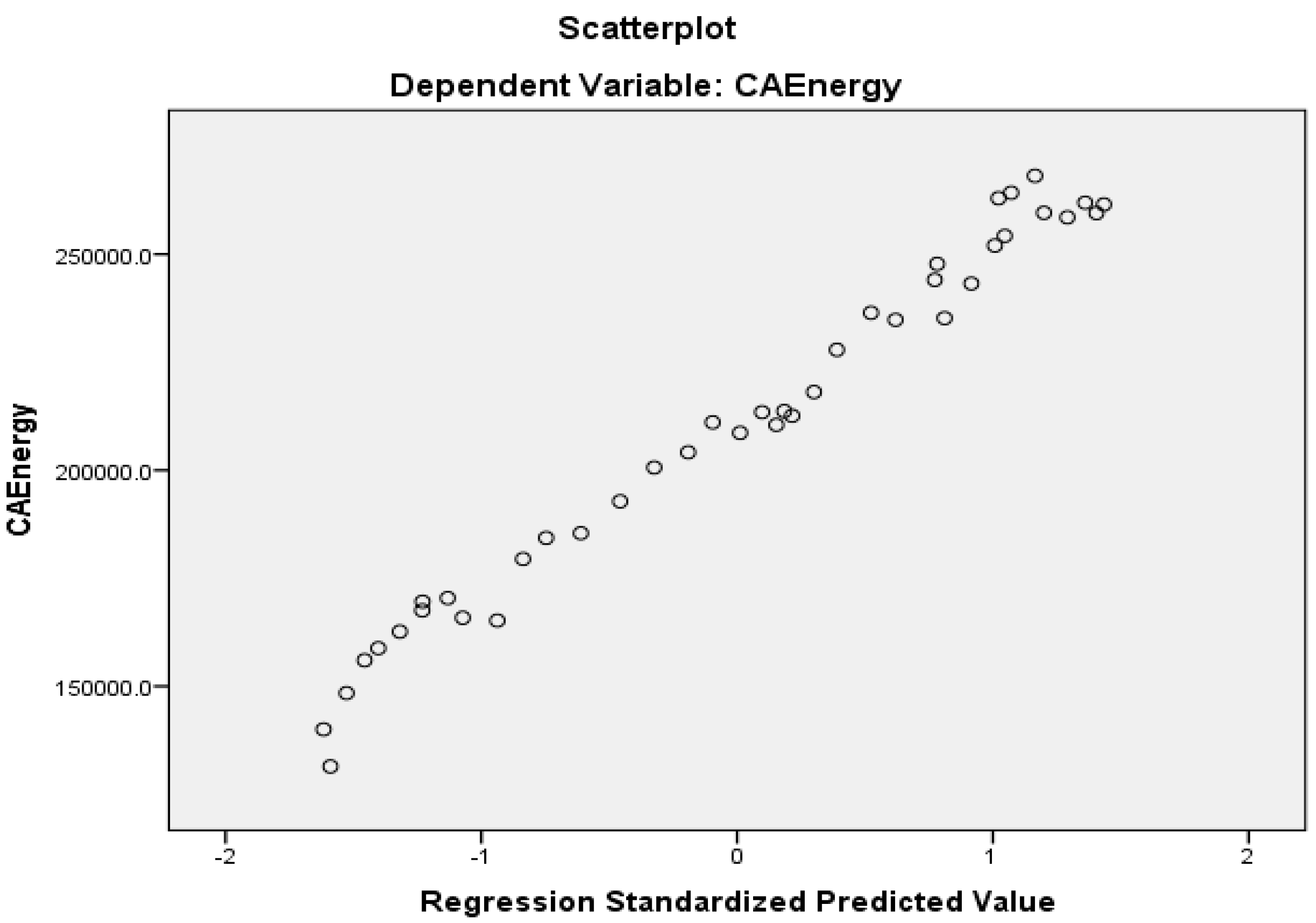
Linear Regression Plots. We used plots to detect any existing outliers and influential cases. We also used plots to validate the assumptions of linearity, equality of variances, and normality. Predicted values, residuals, and other diagnostics are used to plot together with the total energy consumption. The scatterplots were structured in this study by plotting any two of the following: the dependent variable (total energy consumption), standardized predicted values, regression standardized residual, and adjusted predicted values. The plot of the standardized residuals against standardized predicted values is used to validate the linearity and equality of variance.
Table 1 shows the multiple regression analyses for the case of New York (New York), followed by linear regression plots for Case 1 (
Figure 5 and
Figure 6).
Table 2 illustrates the multiple regression analyses for the case of Chicago (Illinois), followed by linear regression scatter plots for Case 2 (
Figure 7 and
Figure 8).
Table 3 illustrates the outcomes of the multiple regressions analysis for the case of Los Angeles (California), followed by various linear regression plots (
Figure 9 and
Figure 10).
All tables listed demonstrate step-by-step backward elimination approaches. All tables present how variables were entered and removed, summarize the models, and report coefficients. Overall, listed tables include information such as the dependent variable (total energy consumption), a list of independent variables (population, electricity average price, average temperature, and extreme weather dummy), criterion for elimination, model summary (R square, constants), coefficients, and the formulated multiple regression models.
Table 1.
New York (New York): multiple regression coefficients a.
Table 1.
New York (New York): multiple regression coefficients a.
| Model | Unstandardized Coefficients | Standardized Coefficients | t | Sig. |
|---|
| B | Std. Error | Beta |
|---|
| 1 | (Constant) | −73,984.734 | 51,835.452 | | −1.427 | 0.162 |
| NYPopulation | 0.007 | 0.003 | 0.254 | 2.224 | 0.033 |
| NYEAP | 992.610 | 196.697 | 0.595 | 5.046 | 0.000 |
| NYCAT | 4051.113 | 2102.691 | 0.172 | 1.927 | 0.062 |
| NYCDummy | −3554.600 | 2703.579 | −0.096 | −1.315 | 0.197 |
| 2 | (Constant) | −64,259.174 | 51,807.644 | | −1.240 | 0.223 |
| NYPopulation | 0.007 | 0.003 | 0.259 | 2.240 | 0.031 |
| NYEAP | 1028.950 | 196.654 | 0.617 | 5.232 | 0.000 |
| NYCAT | 2840.175 | 1908.767 | 0.120 | 1.488 | 0.145 |
| 3 | (Constant) | −43,906.533 | 50,761.324 | | −0.865 | 0.392 |
| NYPopulation | 0.007 | 0.003 | 0.286 | 2.471 | 0.018 |
| NYEAP | 1104.332 | 193.028 | 0.662 | 5.721 | 0.000 |
Figure 5.
Regression standardize residual (New York case).
Figure 5.
Regression standardize residual (New York case).
Figure 6.
Regression standardize predicted value (New York case).
Figure 6.
Regression standardize predicted value (New York case).
Table 2.
Chicago (Illinois): multiple regression coefficients a.
Table 2.
Chicago (Illinois): multiple regression coefficients a.
| Model | Unstandardized Coefficients | Standardized Coefficients | t | Sig. |
|---|
| B | Std. Error | Beta |
|---|
| 1 | (Constant) | −243,481.696 | 20,643.775 | | −11.794 | 0.000 |
| ILPopulation | 0.027 | 0.002 | 0.779 | 14.641 | 0.000 |
| ILEAP | 1020.364 | 213.762 | 0.257 | 4.773 | 0.000 |
| ChicagoAT | 1866.394 | 1050.385 | 0.076 | 1.777 | 0.084 |
| ChicagoDummy | −2398.634 | 1794.215 | −0.058 | −1.337 | 0.190 |
| 2 | (Constant) | −245,932.997 | 20,779.774 | | −11.835 | 0.000 |
| ILPopulation | 0.028 | 0.002 | 0.790 | 14.855 | 0.000 |
| ILEAP | 942.925 | 207.941 | 0.238 | 4.535 | 0.000 |
| ChicagoAT | 1686.340 | 1052.738 | 0.069 | 1.602 | 0.118 |
| 3 | (Constant) | −234,972.174 | 20,021.069 | | −11.736 | 0.000 |
| ILPopulation | 0.028 | 0.002 | 0.804 | 15.021 | 0.000 |
| ILEAP | 941.652 | 212.181 | 0.237 | 4.438 | 0.000 |
Figure 7.
Regression standardize residual (Chicago case).
Figure 7.
Regression standardize residual (Chicago case).
Figure 8.
Regression standardize predicted value (Chicago case).
Figure 8.
Regression standardize predicted value (Chicago case).
Table 3.
Los Angeles (California): multiple regression coefficients a.
Table 3.
Los Angeles (California): multiple regression coefficients a.
| Model | Unstandardized Coefficients | Standardized Coefficients | t | Sig. |
|---|
| B | Std. Error | Beta |
|---|
| 1 | (Constant) | −89,353.913 | 38,621.098 | | −2.314 | 0.027 |
| CAPopulation | 0.009 | 0.001 | 1.225 | 11.819 | 0.000 |
| CAEAP | −1002.423 | 426.248 | −0.241 | −2.352 | 0.024 |
| LosAngelesAT | 2780.130 | 1898.735 | 0.036 | 1.464 | 0.152 |
| LosAngelesDummy | 2430.361 | 2113.047 | 0.029 | 1.150 | 0.258 |
| 2 | (Constant) | −86,711.730 | 38,720.572 | | −2.239 | 0.031 |
| CAPopulation | 0.009 | 0.001 | 1.189 | 11.965 | 0.000 |
| CAEAP | −904.553 | 419.486 | −0.218 | −2.156 | 0.038 |
| LosAngelesAT | 3000.958 | 1897.227 | 0.039 | 1.582 | 0.122 |
| 3 | (Constant) | −28,351.954 | 11,977.546 | | −2.367 | 0.023 |
| CAPopulation | 0.009 | 0.001 | 1.165 | 11.636 | 0.000 |
| CAEAP | −752.236 | 416.275 | −0.181 | −1.807 | 0.079 |
Figure 9.
Regression standardize residual (LA case).
Figure 9.
Regression standardize residual (LA case).
Figure 10.
Regression standardize predicted value (LA case).
Figure 10.
Regression standardize predicted value (LA case).
5.1. Case 1. New York, New York
When the New York population increases by one unit, the total energy consumption increases 0.007 units. When the average price of electricity increases by one unit, the total energy consumption increases 1104.3 units. Although a few extreme weather events occurred during the years 1973–2013, the extreme weather (heatwave) events within the proposed multiple regression model did not impact the total energy consumption statistically, while population and average price of electricity both impacted the amount of total energy consumption (R = 0.91; R Square = 0.829). It is worth noting that here, and in the Chicago, Illinois case below, an increase in price correlates with an increase in consumption. This observation could be indicative of peak demand pricing, during which electricity must be purchased from producers outside a service area because the in service area production has reached its limit.
5.2. Case 2. Chicago, Illinois
When the Chicago (Illinois) population increases by one unit, the total energy consumption increases 0.028 units. When the average price of electricity increases by one unit, the total energy consumption increases 941.6 units. Although a few extreme weather events occurred in Chicago during the years 1973–2013, the extreme weather events within the proposed multiple regression model did not impact the total energy consumption statistically, while population and average price of electricity both did impact the amount of total energy consumption (R = 0.964; R Square = 0.93).
5.3. Case 3. Los Angeles, California
When the Los Angeles (California) population increases by one unit, the total energy consumption increases 0.009 units. When the average price of electricity increases by one unit, the total energy consumption decreases 752.2 units. Although a few extreme weather events occurred in Los Angeles during the years 1973–2013, the extreme weather events within the proposed multiple regression model did not impact the total energy consumption statistically, while population and average price of electricity both did impact the amount of total energy consumption (R = 0.99; R Square = 0.98). Here, a decrease in electricity consumption occurs with an increase in price. This suggests that Los Angeles residents may be motivated to use less energy when it incurs extra cost.
6. Conclusions and Suggestions
Overall, the total energy consumptions of New York, Chicago, and Los Angeles were impacted by changes in population and the average price of electricity. Although we assumed that a higher average electricity price could decrease total energy consumption, only the case of Los Angeles supports this assumption. For the three studied cities, the numbers of identified heat waves are less significant compared to the energy consumption demands of the needs of populations in metropolitan cities. Thus, not only must each city’s economic priorities be considered in developing climate change mitigation strategies, each city’s size and climate must be considered as well.
According to the White House’s Climate Change report [
48], extreme temperature events have increased across the U.S. The year of 2014 was the hottest year globally and the 10 years since 1998 were the warmest years in the world [
48]. In 2012, numerous natural disasters that were induced by weather extremes and/or climate change totaled over $100 billion in losses in the U.S., $30 billion in losses because of droughts and heat waves, $65 billion due to Hurricane Sandy, $11.1 billion due to combined severe weather events, $2.3 billion due to Hurricane Isaac, and $1 billion due to western wildfires [
48]. Vulnerability exists among children, the elderly, and the poor, who were impacted by a variety of stressors associated with public health threats including extreme weather events, air pollution, heat waves, and diseases carried by contaminated water, food, birds and insects.
Carbon dioxide (CO
2) generated 82% of the U.S. greenhouse gas emissions and pollution, methane (CH
4) caused 9% of the U.S. greenhouse gas pollution, nitrous oxide (NO
2) made up 6% of the U.S. greenhouse gas emissions, and fluorinated gases produced 3%. Carbon dioxide is produced because of solid waste, trees, fossil fuels (coal, oil, and natural gas), and chemical particles. Methane is caused by the procedures of transportation and production of coal, oil, landfills, and natural gas. Nitrous oxide is produced because of industrial and agricultural activities and combustion of fossil fuels and solid waste. Fluorinated gas is produced during industrial processes [
48].
Power plants generated one-third of all domestic greenhouse gas pollution. Several areas of progress have been highlighted by the White house [
48] and the President’s Clean Power Plan. For example, U.S. greenhouse gas pollution recently hit its lowest level in 20 years. The efficiency of cars and trucks will be doubled by 2025, benefiting from the highest fuel economy standards in the U.S.
Over the latest decade, energy-related progress has drawn the significant attention of researchers and policymakers, including enhancement of renewable energy deployment, decreased carbon dioxide emissions, advanced energy technology, increased oil and gas production, and effective risk control of the energy infrastructure and manufacturing in the United States. The Department of Energy in the U.S. is exploring a variety of research and development opportunities to enable advanced tools and science for technology innovations integrated with the goals of spurring the pace of sustainability, prevention, resilience, and reliability.
Through updating innovative energy infrastructure, evaluating cost-effective energy consumption, employing clean energy, and reducing greenhouse gas emissions, it is possible to mitigate the outcomes of climate change and sustain the quality of life for future generations. Because of the benefits of implementing sustainable business models, innovative policy, and technology advancement, further research that aims to investigate the relationships among viable attributes that affect energy consumption behaviors can provide strategic plans and make contributions to the literature as well as to climate change adaptation.
Adopting advanced technologies may increase the efficiency, sustainability, stability, and diversity of energy supplies, coupled with the benefits of possible reduced energy prices. Various firms and research centers strive to provide the methodologies and strategies to reduce the capital, operational costs and fuel prices of natural gas, domestic oil, hydrogen, and electricity through adopting innovative technologies of installing and operating wind turbines, green lighting, and photovoltaics. Additionally, modernizing communities’ lifestyles and changing individuals’ behaviors and habits may lower energy consumption costs, reduce footprints, minimize pollution (water, land, and air) caused by energy production and consumption, and benefit both individual households and the economy as a whole.
The first limitation of this study was that we mainly focused on the heat wave indicator. The second main limitation was that we did not include the impacts of possible island-effects on the total electricity consumptions within the models. The third limitation was that we mainly used the identified annual data sets due to the availability of specified data sets. Future research may consider disaggregate the annual data sets into monthly data sets to capture the variances due to seasonality. Researchers may consider categorizing catastrophic heat waves or extreme snowstorms as dummy variables to investigate how listed dummy variables could affect total energy consumption, including any public intervention strategies during significant inflation/deflation periods to examine how price policy could impact overall energy consumption. Including island-effect facts and other econometric factors related to development status would be useful for investigating the relationship between energy consumption, recessions/economy, and adaptation to climate change.


