Opportunity Costs of Carbon Emissions Stemming from Changes in Land Use

Abstract

The REDD (Reducing Emissions from Deforestation and Forest Degradation) mechanism allows carbon sinks to be used as carbon credits in order to offset emissions from other sources. However, this practice has raised a number of issues relating to financial incentives. In this study, we develop a spatially explicit model for predicting carbon emissions from deforestation that meet baseline levels as well as farmers’ opportunity costs (measured in US dollars per ton of CO2e) under three temporal scenarios with several potential discount rates for agricultural income. Additionally, we use two different accounting methods recommended by the Intergovernmental Panel on Climate Change (IPCC), including the average storage method and the “ton-year approach,” to evaluate emissions reductions. We find that farmers are more likely to prefer REDD in the short-run when discount rates are higher than 10%. However, further analysis indicates that opportunity costs would increase significantly over longer periods of time (middle-term schemes of 35 years or long-term schemes of 55 years), thereby dissuading farmers from choosing REDD. Our findings highlight the drawbacks in using REDD to mitigate global climate change and conserve forests based on farmers’ financial incentives.

1. Introduction

Tropical forests play a significant role in the global carbon budget [1,2,3] because they contain as much carbon in their vegetation and soils as all temperate-zone and boreal forests combined. The Fifth Assessment Report (AR5) from the International Panel on Climate Change (IPCC) now estimates that emissions from forestry may constitute less than 10% of total emissions, which is significantly less than their former estimate of 17.4% [4,5]. Conversely, CO₂ emitted from land use, land use change, and forestry activities (LULUCF) constitutes approximately one-third of developing countries’ total emissions [6]. The country with the largest volume of emissions from land use change is Indonesia, which emits 34% of the global total [7]. The Kyoto Protocol (which is widely regarded as the first step toward a truly global emission reduction regime that would stabilize greenhouse gas (GHG) concentrations) did not address the clearing of forests for plantations (such as oil palm, rubber, and cacao), despite the fact that it is the main source of released carbon from land use change. Such failures to address tropical forests and their deforestation in international emissions reduction schemes may be hindering efforts to mitigate global climate change. This concern was addressed during the 15th Conference of the Parties (COP15) at the 2009 United Nations Climate Change Conference in Copenhagen, where the parties agreed upon a program focused on reducing emissions from deforestation and forest degradation (REDD) in developing countries through positive incentives. The COP16 in Cancun, yielded an agreement further addressing REDD that is expected to revitalize the program by increasing funding readiness and invigorating donor pledges, which now amount to nearly US$5 billion. The general consensus at Doha in 2012, was that there had been mixed results regarding the financing, safeguards, measurement, reporting, and verification of REDD; in fact, it was widely recognized that the only significant progress that had been made had been in the field of reference level technology. In the COP19 in 2013, a package of decisions were made (termed “The Warsaw Framework”) on the UN-backed scheme that aimed to reduce emissions from deforestation and forest degradation, thereby completing the Cancun agreements. The Warsaw Framework emphasized that financing, which is one of the most fundamental challenges to REDD, should be “results-based” and that developing countries should obtain financing from funding agencies, such as the Green Climate Fund, or other sources.

Another issue that has been hotly debated in previous conferences is the measurement, reporting, and verification (MRV) of forest reference levels (defined as expected or business-as-usual, year-over-year emissions from deforestation and forest degradation in the absence of additional reduction efforts). The Warsaw Framework formalized this process because the COP realized that verification is vital to incentive-based funding.

A typical REDD proposal seeks to reduce GHG emissions and support sustainable development while minimizing costs [8,9]. REDD payments are granted so that recipients may create a development mechanism that will slow deforestation and promote sustainable forest management, ultimately reducing carbon emissions and improving ecosystem services. Although details regarding the manner in which a REDD mechanism might be incorporated have yet to be decided, there are some basic components that will undoubtedly be incorporated in the final mechanism; these include carbon accounting, baselines, emission reduction strategies, monitoring, verification, and the funding for emission reductions. Various actors are involved in either the implementation, policy-making, or financial aspects of each of these processes (Figure 1) [10].

Figure 1. Mechanisms and actors involved in reducing emissions from deforestation and forest degradation (REDD).

Figure 1. Mechanisms and actors involved in reducing emissions from deforestation and forest degradation (REDD).

Costs, which vary based on the approach used and the types of costs considered, play a key role in REDD. Generally speaking, REDD costs may be classified into five categories including opportunity, implementation, administrative, transaction, and stabilization costs [11]. Among these, opportunity costs are usually the single most important and the largest component of total costs. Thus, in order to develop policy priorities and enter into REDD agreements, it is necessary to acquire information on these costs at a local level. The general process for estimating opportunity costs involves three main steps: (I) identifying and mapping the areas at risk of being deforested or degraded and the land uses that are most likely to replace them; (II) estimating the returns to both forest areas and alternative land uses as well as the carbon stock for each (to whatever extent possible, other benefits should be measured as well); (III) using these data to make opportunity cost and carbon emissions projections under alternative scenarios [11].

Analyzing opportunity costs would provide insight into the drivers and causes of deforestation, identify REDD’s potential effects on different social groups, help estimate forest owner’s compensation for changing their land use, and improve estimates of the other REDD costs [12,13,14]. The Warsaw Framework in COP 19 grants to national governments the decision on dealing directly or indirectly with such costs, through projects, programs or other mechanisms. Consequently, we believe that our work on this subject will be particularly useful to national policy makers in their implementation of REDD projects.

There are four methods that have been used to the estimate the opportunity costs of land usage [15,16]:

(I)

Local/micro-level empirical data estimates: these are based on empirical data, are region specific, and reflect local conditions and costs.

(II)

Generic or average production cost estimates: are calculated using data from other countries.

(III)

Land price estimates: reflect the discounted stream of returns from the most productive use of land.

(IV)

Global partial equilibrium model estimates: simulate relevant parts of the world economy (including the forest, agriculture, and energy sectors) to estimate supply curves for emissions reductions.

Gregersen et al. [12] presented six main drawbacks to these methods: they have difficulty accounting for illegal activities; they do not adequately account for the payments needed to halt deforestation; the analyses are not carried out in well-functioning market systems; prices are likely to be set by the carbon offset markets rather than various forest owners’ and users’ opportunity costs; the estimates are dependent upon the approach used; and they fail to account for the dynamics of opportunity costs.

Table 1 summarizes a range of estimates of REDD opportunity costs based on different sources and methodologies. The estimation approach utilized in this study is similar to that presented in the Stern Review and those of global partial equilibrium models of the forest sector.

Table 1. REDD opportunity costs from different sources ($/ton CO2e).

Research Area	Average	High	Low	Source
Global	12.32	17.86	6.77	Boucher [16]
Global	5.52	8.28	2.76	Stern [17]
Tanzania	10.5	12	9	Tom Blomley and Timm Tennigkeit [18]
Indonesia	21.65	33.44	9.85	Venter et al. [19]
Indonesia	3.15	4.66	1.63	Venter et al. [19]
Indonesia	13.45	19.24	7.66	Butler et al. [20]
Brazil	9.1	11.5	6.7	IIED [21]

Table 1. REDD opportunity costs from different sources ($/ton CO2e).

Research Area	Average	High	Low	Source
Global	12.32	17.86	6.77	Boucher [16]
Global	5.52	8.28	2.76	Stern [17]
Tanzania	10.5	12	9	Tom Blomley and Timm Tennigkeit [18]
Indonesia	21.65	33.44	9.85	Venter et al. [19]
Indonesia	3.15	4.66	1.63	Venter et al. [19]
Indonesia	13.45	19.24	7.66	Butler et al. [20]
Brazil	9.1	11.5	6.7	IIED [21]

Schlamadinger and Marland [22] have indicated that sequestering carbon in the biosphere might be different from reducing GHG emissions from fossil fuels in one fundamental way; the carbon in sinks within the biosphere may not remain there. Carbon sinks, which result from the discontinuation of forestry activities, may act over only short periods of time, and consequently, these sinks do not provide the same long-term benefits as the abatement of GHG emissions. Several approaches have been suggested that treat carbon sinks in much the same way as the sequestration effect of fossil fuels [23,24,25,26,27,28]. Therefore, opportunity cost estimations could be influenced by the choice of these approaches. As such, for this study, we developed a spatially explicit model to predict the carbon emissions from deforestation that meet baseline levels as well as farmers’ opportunity costs (measured in US dollars per ton of CO2e) under three temporal scenarios with several potential discount rates for agricultural income. We also used two accounting methods recommended by the Intergovernmental Panel on Climate Change (IPCC): (I) the average storage method and (II) the “ton-year approach.” We then conducted a case study on Central Kalimantan, Indonesia where we evaluated farmers’ financial incentives for participating in REDD.

2. Methods

2.1. Baseline Modeling

A REDD “baseline” is defined as “an expected, or business-as-usual (BAU), emission of CO2e (greenhouse gases measured as equivalent units of carbon dioxide) from deforestation and forest degradation in the absence of additional efforts to curb such emissions” [29]. Such baselines are critical for assessing an emission reduction operation as well as for negotiating meaningful targets. Therefore, one of the key tasks of REDD is to determine feasible, transparent, and sound deforestation emission baselines and accounting rules [30].

In this study, the baseline was calculated by combining the BAU scenario with a bookkeeping carbon-cycle model. An improved cellular automaton (ICA) system, in which a cell in a regular grid changes to a finite number of possible states according to a local interaction rule [31,32], was utilized to predict land use changes. Cellular automaton models have proven to be quite useful due to their operationality, simplicity, and ability to embody both logic- and mathematics-based transition rules, thus enabling complex patterns to emerge directly from the application of simple local rules. These models provide powerful simulation environments that are represented by a grid of spaces (or a raster) in which the consequences of trends and policy interventions are depicted with dynamic year-by-year land use maps. In this study, the process of land use transition within a cell was determined by six factors:

(1)

State of each cell as represented by spatial variables (e.g., the various land use types).

(2)

Probability of land conversion.

(3)

Physical suitability, which describes the degree to which the cell was suitable for use as a plantation based on its elevation, slope, aspect, and soil type.

(4)

Spatial constraints that prohibit the cell from being converted to certain land use types, which assures that deforestation does not occur in certain prohibited areas.

(5)

Accessibility, which describes the ease with which a plantation can fulfill the cell’s needs for transportation and mobility given the underlying transportation system (e.g., distances to rivers, roads, and villages).

(6)

Each cell’s neighborhood, which represents the impact of land use from all cells surrounding the focal cell. The Moore neighborhood was adopted in this study and eight neighbors were used.

ICA requires validation within a neighborhood context because even maps that do not precisely match on a cell-by-cell basis could still present similar spatial patterns and agreements within the vicinity of certain cells. In order to address this issue, we adjusted the weights of all of the spatial interaction rules according to reliable historical land use data [33,34]. The calibration procedure was conducted in two steps: First, overall dynamics, system-wide features, and land use patterns were verified. Next, we fine-tuned the information in order to acquire as much spatial detail and pattern similarity as possible at the cellular level [35]. In order to validate our results, we utilized Kappa statistics as goodness-of-fit measures so as to compare the simulated and actual maps.

The estimation of carbon emissions from deforestation activities, which is based on a bookkeeping carbon-cycle model, is similar to the process-based approach recommended by the IPCC [36]. The model tracks year-to-year changes in carbon stocks due to deforestation, forest regeneration, permanent clearing of forests, and forest decay [37,38,39,40].

In this study, carbon fluxes caused by tropical deforestation were allocated into three different carbon pools [40]: (I) the immediate release of carbon into the atmosphere from plant material as it was burned, including biomass from deforestation and biomass from cleared secondary vegetation at the time of clearing, (II) the slower release of carbon from the decay of slash, product, and elemental carbon pools, and (III) the accumulation of carbon during regrowth. The net carbon fluxes were calculated as the sum of the individual fluxes according to the following equation:

$$C_{f,net}(t)=C_{f,burn}(t)+C_{f,decay}(t)+C_{f,regrowth}(t)$$

(1)

where t represents the year; C_f,net(t) is the total carbon flux; C_f,burn(t) is the carbon flux from instantaneous burning; C_f,decay(t) is carbon flux from the decay of product, slash, and elemental carbon pools; and C_f,regrowth(t) is carbon flux caused by plant regrowth. Here, C_f,decay(t) can be calculated as:

$$C_{f,decay}(t)={\lambda }_{slash}{C}_{slash}(t-1)+{\lambda }_{prod}{C}_{prod}(t-1)+{\lambda }_{elem}{C}_{elem}(t-1)$$

(2)

and C_f,burn(t) can be calculated as:

$$C_{f,burn}(t)=Bi{o}_{clear}(t)f_{burn}$$

(3)

Joeni’s [41] biomass values, which were obtained from in situ forest inventories and permanent sampling plots, were selected as our initial values. We also assumed that (I) the fraction of the initial carbon in the slash, product, and elemental carbon pools decayed at a rate of 10%, 10%, and 0.1%, respectively; (2) secondary vegetation accounted for 20% of the total forest area, and that (3) regenerating forests recovered 30% of their original biomass in 25 years and another 10% over the next 50 years. Figure 2 shows carbon fluxes per unit in the book-keeping carbon cycle model.

Figure 2. Carbon fluxes per unit in the book-keeping carbon cycle model.

Figure 2. Carbon fluxes per unit in the book-keeping carbon cycle model.

2.2. Opportunity Costs

The key objective for any project under REDD is to determine the expected cost per-unit of averted GHG emissions (i.e., the opportunity cost). We used the following equation to calculate the opportunity cost, which was measured in dollars per ton of CO2e emissions avoided:

$$Opportuni{y}_{\cos ts}=NPV/Carbo{n}_{emissionss}$$

(4)

where NPV represents the net present value of agricultural income. NPV must be calculated in order to determine the sum of all future benefits in today’s terms. In this study, NPV was calculated based on revenue from four main sources: (I) logging (one-time), (II) rice cultivation, (III) rubber plantations, and (IV) oil palm plantations. The NPV of the community’s total revenue was calculated as [42,43]:

$$NPV=V_1+{\theta }_s{{\displaystyle \sum _{t=0}^T(1/(1+\gamma ))}}^t\times V_s+{\theta }_g{{\displaystyle \sum _{t=0}^T(1/(1+\gamma ))}}^t\times V_g+{\theta }_p{{\displaystyle \sum _{t=0}^T(1/(1+\gamma ))}}^t\times V_p$$

(5)

where T is the forest protection commitment period; V₁, V_s, V_g, and V_p are the net revenues per hectare of logging, rice cultivation, rubber plantations, and oil palm plantations, respectively; γ is the discount rate; and θ_s, θ_g, and θ_p are the ratios of rice cultivation, rubber plantations, and oil palm plantations to the total area of expanding agricultural land. V_s took into account the sum of all rice produced by individual farmers, the price of rice, labor costs of rice production, and the total agricultural land dedicated to rice production. V_g was calculated in a similar fashion. V_p was obtained using Fairhurst and McLaughlin’s [44] cash flow model and a crude palm oil (CPO) price of US$500 USD/ton, which is close to the present and long-term discounted prices. Fairhurst and McLaughlin [44] estimated planting and operating costs by interviewing financial and management staff at seven estates in Kalimantan. In this model, harvest, transport, and factory processing, as well as all committed overhead costs (e.g., farm, factory, and general costs) were taken directly from one of the estates visited.

We assumed that the rubber yield would increase in the 11th year of planting and that oil palm yield would increase in both the third and 10th years (which is when palm trees reach maturity, though they decrease slightly around their 25th year). Table 2 lists all of the parameters, descriptions, and values used in estimating agricultural revenue.

The discount rate, which is a measure of time preference, was used to “convert” future cash flows into present values. Consequently, a higher discount rate translated to lower future REDD benefits. If a REDD project were to have a long payback period, the discount rate would significantly influence the present value of future profits, and as a result, the NPV. The discount rate varies from region to region because it depends on interest and inflation rates as well as on the risks of the REDD project (as they are perceived by the investors and held constant over time). Smith [45] suggested that the choice of discount rate depends on whether (I) the policy question is marginal or non-marginal (when a policy problem is non-marginal, welfare economics must directly compare the different paths’ present welfare values, which are calculated using the discount rate that is consistent with each path, given its consumption growth rate); (II) social or private preferences are considered (the private discount rate invariably exceeds social discount rates because society places greater value on the welfare of future generations than individuals do); and (III) the country is developed or developing (in developing countries, the discount rate should be higher as the present generation can be expected to be significantly poorer than future ones, whereas the generational gap in welfare is more limited in developed countries). It has been suggested that, in developing countries, the discount rate could be as high as 10%–12% as compared to 4% in developed countries [46]. Sathaye et al. [47] applied a discount rate of 12%–19% for short rotation forestry in Africa and Latin America. On the other hand, Hunt [48] proposed a sustainable discount rate of 8% for the least developed countries, and Camino et al. [49] used rates ranging from 4% to 16% for teak in Central America. Based on these studies, we used three reasonable discount rate scenarios: 2.5%, 5%, and 10%. These scenarios were combined with three REDD project durations, including 15-year, 25-year, and 55-year time spans, in order to examine the effects of opportunity costs on REDD.

Table 2. Parameters, descriptions, and values used in estimating agricultural revenue.

Parameter	Description	Value	Source
V1	One-time net revenue from logging per hectare	830 US$	Yamamoto et al. [43]
Vg	Net revenue from rubber plantations per hectare	75.1 US$	Yamamoto et al. [43]
Vp	Net revenue from oil palm plantations per hectare	258.27 US$	Fairhurst and McLaughlin [44]
θs	Percentage of rice cultivation in the total area of expanding agricultural land	16.3%	Field survey
θg	Percentage of rubber plantations in the total area of expanding agricultural land	32.7%	Field survey
θp	Percentage of oil palm plantations in the total area of expanding agricultural land	51%	Field survey
P3	Price of rice	0.32 US$/kg	Yamamoto et al. [43]
Pg	Price of rubber	0.87 US$/kg	Yamamoto et al. [43]
W	Minimum wage	0.68	Yamamoto et al. [43]

Table 2. Parameters, descriptions, and values used in estimating agricultural revenue.

Parameter	Description	Value	Source
V1	One-time net revenue from logging per hectare	830 US$	Yamamoto et al. [43]
Vg	Net revenue from rubber plantations per hectare	75.1 US$	Yamamoto et al. [43]
Vp	Net revenue from oil palm plantations per hectare	258.27 US$	Fairhurst and McLaughlin [44]
θs	Percentage of rice cultivation in the total area of expanding agricultural land	16.3%	Field survey
θg	Percentage of rubber plantations in the total area of expanding agricultural land	32.7%	Field survey
θp	Percentage of oil palm plantations in the total area of expanding agricultural land	51%	Field survey
P3	Price of rice	0.32 US$/kg	Yamamoto et al. [43]
Pg	Price of rubber	0.87 US$/kg	Yamamoto et al. [43]
W	Minimum wage	0.68	Yamamoto et al. [43]

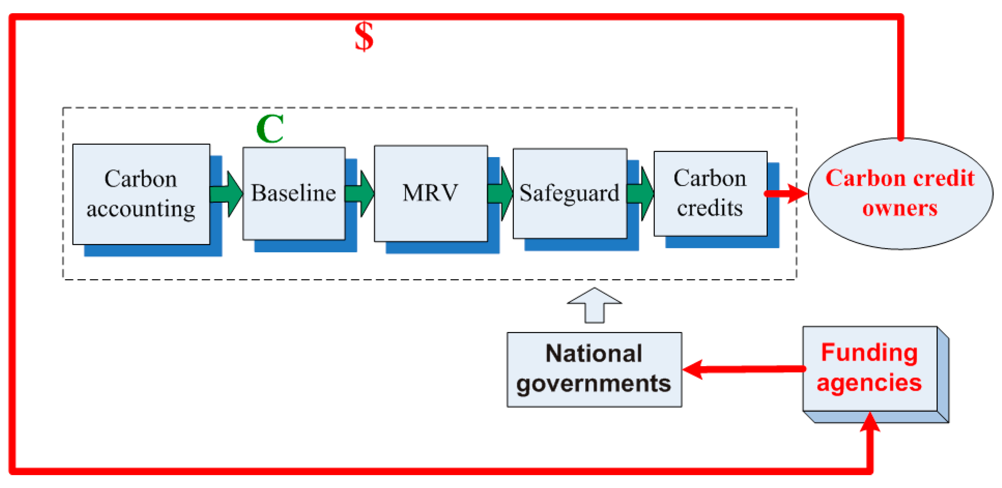
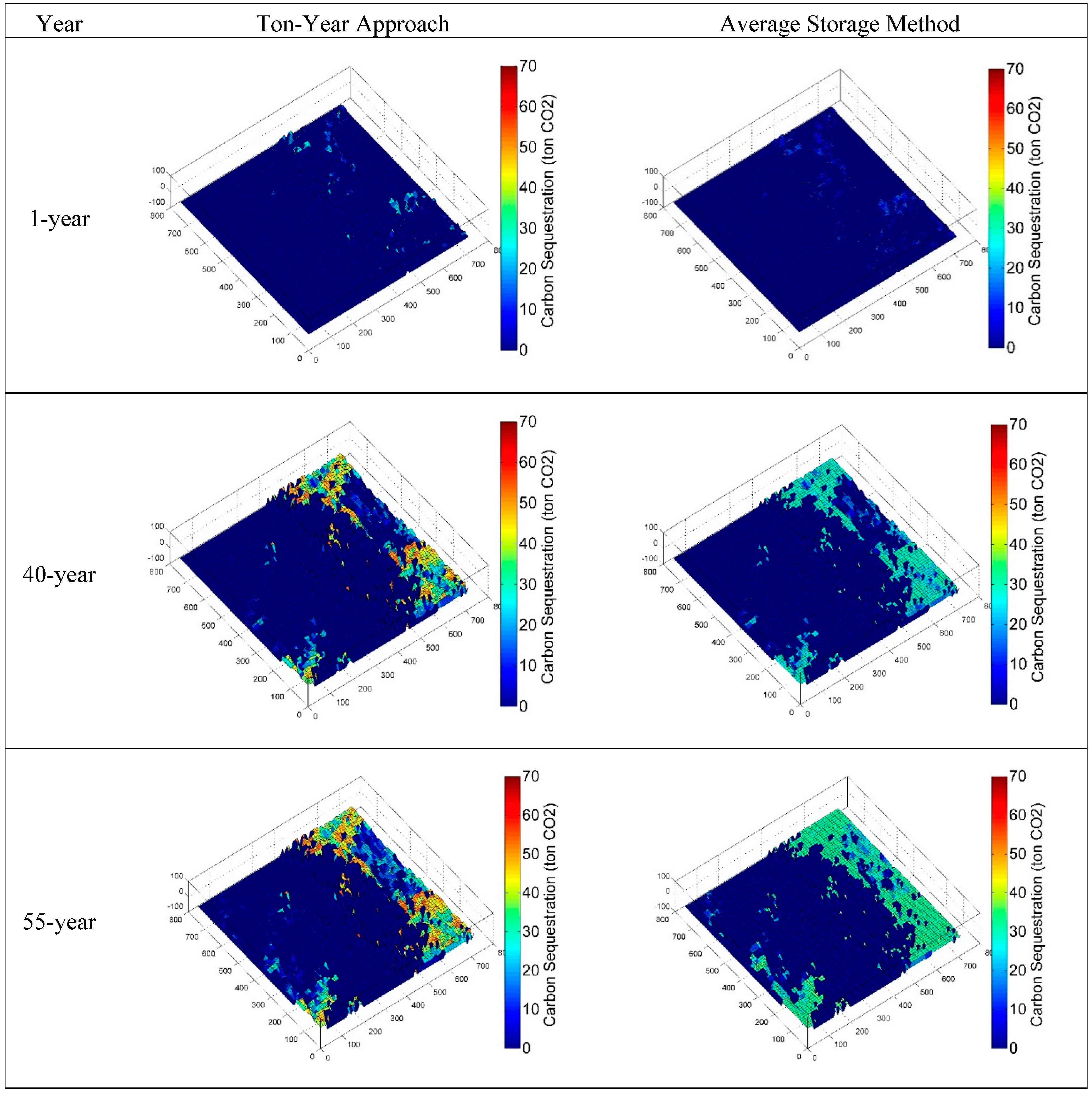
2.3. Accounting Methodology

Under the average storage method, the amount of carbon stored in a site is averaged over the long-run according to the following equation:

$$\overline{C(t)}=({\int }_0^{TH}XP(t)d_t-{\int }_0^{TH}XB(t)d_t)/T$$

(6)

where t is time, TH is the time horizon, XP is the carbon stored as part of the project, XB is the baseline carbon storage, T is the project duration, and all of the measurements are expressed in tons of carbon per hectare [50]. The advantage of this method is that it accounts for the dynamics of carbon storage over the duration of the entire project, not just for the times chosen for accounting [4].

Under the ton-year approach, carbon credits, which are directly proportional to the project’s timeframe, are assessed as the environmental and economic benefits of limited-term sequestration [28,51]. Based on this approach, it should be possible to define some measure of “equivalence” between temporary credits and permanent reductions that can be used to compare their effectiveness [52]. An equivalence factor (Ef), through which the climatic effect of temporal carbon storage could be converted to an equivalent amount of avoided emissions, can thus be calculated within a range of 0.007–0.02 [24,53]. This parameter may be derived from the “equivalence time” concept (referred to as Te), which Costa and Wilson [54] calculated using the following steps:

Step 1. The absolute global warming potential (AGWP) of CO₂ is calculated according to the following equation [55]:

$$AGWP\left(C{O}_2\right)={\int }_0^{TH}{a}_x\times [C{O}_2(t)]d_t$$

(7)

where TH is the time horizon, ax is the climate-related radiative forcing caused by a unit increase in the atmospheric concentration of CO₂, and [CO₂(t)] is the time-decaying quantity of a pulse of emitted CO₂. This last variable is derived from the following formula [56]:

$$F\left[C{O}_2\left(t\right)\right]=0.30036e^{-t/6.6993}+0.34278e^{-t/71.109}+0.35686e^{-t/815.727}$$

(8)

where t is the year.

Step 2. In Equation (1), the integral is proportionate to the cumulative radioactive forcing exerted by a unit of CO₂. In Equation (2), the integral of the decay curve is equivalent to the forcing effect of approximately 55 ton-years of CO₂ over the 100-year reference period established by the Kyoto Protocol. Thus, Te, which is the length of time that CO₂ must be stored as carbon in either biomass or soil for it to prevent the cumulative radiative forcing effect exerted by a similar amount of CO₂ during its residence in the atmosphere, is 55 years. As a result, Ef (the ton-carbon-year factor) is equal to 1/Te or 0.0182 tons of avoided CO₂ emissions.

Step 3. Finally, for each ton of carbon stored in a given year, the project receives credit for 0.0182 tons of carbon. This means that the fraction of awarded credit can be calculated based on the ratio of the project’s duration to the equivalence time.

2.4. Market Price of Carbon

In this study, we utilized the market carbon price, which is derived from Nordhaus’ [57] dynamic integrated model of climate and the economy (DICE). DICE is a top-down, macroeconomic model that estimates the cost of carbon based on the price that would be necessary to raise fuel costs and thereby predicts the cost that would be necessary to reduce emissions to a targeted level. Nordhaus noted that the DICE baseline temperature projections were in the lower-middle range of those analyzed in the IPCC’s Fourth Assessment Report, which estimated that the global mean temperature would increase between 1.8 °C and 4.0 °C from 1980–1999 to 2090–2099; the DICE baseline predicted a global mean temperature increase of 2.2 °C over this period, resulting in several different scenarios [57]. Considering the two recent global financial crises in 2007 and 2010, we adopted the scenario in which Annex I countries (including the United States) collectively would agree to reduce their GHG emissions by an average of 5.2% from 2008 to 2012 (i.e., original version of the Protocol). As such, the carbon price was set at $15.02 per unit of CO2e after three years, increased to $15.72 after 13 years, and then reduced to $14.74 after 23 years, resulting in an average carbon price of $14.00. According to State of the Voluntary Carbon Markets [58], the current real average price (volume-weighted $/tCO2e) is $6.05. Consequently, we proportionally adjusted the future average carbon price from the DICE model to $5.64 for our study.

3. Results

We examined the opportunity costs used for REDD in Central Kalimantan, Indonesia. This province contains rapidly expanding palm plantations, with 763,000 ha of forest threatened by future plantation expansion plans [59]. Our study area consisted of 47,940.75 ha in a 22.5 km × 21.5 km square area located in the southeast region, north of Palangka Raya (Figure 3). Historically, this area was covered by heath forests and peat swamps; however, since 2000, this area has been plagued by large-scale deforestation. Studies [60] have indicated that the remaining forest can be categorized as “Forest Frontier,” the clearance of which is predicted to reach a maximum in the next 30 years while palm plantations expand. Landsat images of this area captured in 2000, 2005, and 2009 were categorized based on their depicted land use (dense forest, peat, sparse forest, plantation, road, or water) through supervised classification. Conversions of dense forest, peat, and sparse forest were classified as “deforestation.” By using the ICA system to compare the simulated and historical land-use maps, we found that the Kappa coefficient between the two was approximately 0.65. We then compared the results over the three project durations.

Figure 3. Location of study area in Central Kalimantan, Indonesia (Map source: Wikipedia; photos: Heli LU).

Figure 3. Location of study area in Central Kalimantan, Indonesia (Map source: Wikipedia; photos: Heli LU).

Figure 4 illustrates the spatial evolution of carbon sequestration in the study area over a 55-year period. Terrestrial areas capable of high carbon sequestration tended to be flatter and near water sources and roads. These areas were at high risk of deforestation and therefore critical to meeting emission reduction targets, which made them of utmost importance to REDD. If the government cannot properly identify and target areas such as these, then it will need to compensate for a larger area in its efforts to avoid deforestation, which will ultimately raise the cost of such efforts [15].

Figure 4. Time-series distribution of carbon sequestration over a 55-year period as predicted by the average storage method and the ton-year approach. Areas of high carbon sequestration are depicted in yellows and reds, areas of low sequestration are shown in light blue, and the background areas are dark blue.

Figure 4. Time-series distribution of carbon sequestration over a 55-year period as predicted by the average storage method and the ton-year approach. Areas of high carbon sequestration are depicted in yellows and reds, areas of low sequestration are shown in light blue, and the background areas are dark blue.

Information on the speed and direction of deforestation is integral to anticipating future threats to carbon stocks. By identifying, characterizing, and mapping hotspots, precise information on a region’s vulnerability to deforestation could be used to improve conservation plans and budgets [54].

As shown in Figure 5, the two accounting methods differed significantly in their carbon values despite the fact that they had identical future land use distributions. This is mainly because we measured carbon sequestration as a complex response to the different accounting systems. For example, the average storage method involves frequent exchanges of carbon credits and debts between project developers and buyers or regulatory bodies, while the ton-year approach takes into account the time dimension of carbon sequestration and storage [54]. Due to these complex processes and purposes, carbon values differ considerably under the different accounting systems.

Figure 5. A comparison of opportunity costs.

Figure 5. A comparison of opportunity costs.

We also explored the effect of project duration on opportunity costs. It should be noted that if agricultural profit is linear (i.e., constant over time), then the different project durations should have exactly the same values, and therefore, not affect opportunity costs. However, they are usually temporally heterogeneous. For example, the cost of delivering a ton reduction in CO₂ emissions varied from US$8.6–US$23.4 (Table 3) based on the scenario. Furthermore, the choice of discount rate also had an impact; for a long-term project, in which spending would have to be maintained for 55 years in order to permanently reduce emissions, the costs fell by approximately US$14.0 per ton of CO2e when the discount rates increased from 2.5% to 10%.

We determined that farmers were likely to prefer short-term REDD schemes when discount rates were higher than 10% because the opportunity costs would all be below the average carbon price of $5.64 per CO2e. Conversely, in the medium- and long-term schemes, opportunity costs would exceed the average price due to significant accumulations in agricultural profits and weak increments in carbon prices.

Table 3. Opportunity costs based on different carbon accounting methods and project durations.

Accounting Method	Scenario	Opportunity costs (US$/ton CO2e)
		2.5% Discount	5% discount	10% discount
Ton-year approach	Short-term scheme: 15-year	14.7	13.9	5.8
	Medium-term scheme: 25-year	19.6	14.5	7.5
	Long-term scheme: 55-year	23.4	15.4	8.5
Average storage method	Short-term scheme: 15-year	8.6	8.1	5.5
	Medium-term scheme: 25-year	14.6	10.9	7.1
	Long-term scheme: 55-year	21.4	14.1	7.8

Table 3. Opportunity costs based on different carbon accounting methods and project durations.

Accounting Method	Scenario	Opportunity costs (US$/ton CO2e)
		2.5% Discount	5% discount	10% discount
Ton-year approach	Short-term scheme: 15-year	14.7	13.9	5.8
	Medium-term scheme: 25-year	19.6	14.5	7.5
	Long-term scheme: 55-year	23.4	15.4	8.5
Average storage method	Short-term scheme: 15-year	8.6	8.1	5.5
	Medium-term scheme: 25-year	14.6	10.9	7.1
	Long-term scheme: 55-year	21.4	14.1	7.8

In the study area, cleared forest lands may initially be unprofitable, but would gradually become more lucrative after they were switched to particular time profile activities, such as rice cultivation, rubber plantations, or oil palm plantations. Even if yields remained unchanged, their value could increase over time as input and output prices change. These factors will affect the present value of the projected flow of different land uses’ costs and benefits, and hence, the opportunity costs of avoiding deforestation under REDD.

Sensitivity analyses were conducted by changing oil palm and rubber plantations’ values by about 10%. This method allowed us to identify the parameters that exerted greater effects on the modeling results. The sensitivity analysis can further reveal how specific plantations would influence opportunity costs if input values were changed, and thus, it may be useful in targeting incentives. For each parameter change, the percentage impact on the opportunity costs was recorded and shown graphically in the form of a tornado diagram (Figure 6). It can be seen that the change in opportunity costs is only about 13.3% when rubber plantations are increased by 10%. In contrast, it changes by a noteworthy 30.52% when oil palm plantations are increased by the same factor.

Figure 6. Sensitivity analysis.

Figure 6. Sensitivity analysis.

4. Discussion

The revenue from the restrictions on productive activities in forests should be considered in the development of REDD projects. Without proper compensation, local governments will have no incentive to support REDD, as they would face forgone taxes, fees, and shared-revenue, while receiving almost no benefits [61]. Financial incentives for REDD, at the very minimum, should compensate for the cost of its implementation, including opportunity costs [16,62,63]. Opportunity costs could provide REDD project planners and government agencies with vital information on (I) deforestation and forest degradation drivers, (II) the agencies affected by REDD projects, and (III) the level and scope of REDD compensation.

The estimates reviewed in this study are consistent with those of global partial equilibrium models of the forest sector. Although the values we found are nearly double those presented in the Stern Review, these abatement options are more cost effective than many non-forestry sector abatement options (e.g., solar energy, wind energy, and carbon capture and storage). Thus, it can be seen that preventing deforestation and forest degradation is one of the cheapest options for mitigating emissions.

In this study, we determined how specific plantations affect the implementation of REDD projects through a sensitivity analysis. Our results indicated that opportunity costs increase significantly as palm oil plantations increase, while rubber plantations (as they currently stand) have little effect. This finding is of particular relevance to Central Kalimantan, where plans to expand oil palm plantations are threatening forests. In recent years, a sharp increase in the price of crude palm oil has driven this area to dramatically expand its cultivation of oil palm. Our research provides a strong perspective for local policymakers on the evaluation of field potentials when accounting for the financial incentives of REDD.

On the whole, we demonstrated that the opportunity cost of reduced emissions can be affected by the choice of discount rate and may vary over time. Therefore, our findings highlight the need to consider both project duration and the discount rate when determining appropriate financial supports for reducing GHG emissions related to deforestation and forest degradation in developing countries. We believe that the compensation for carbon credits in REDD projects cannot be treated in isolation and must account for a variety of factors, such as carbon accounting, project duration, and the discount rate. We further contend that comprehensive approaches for dealing with carbon dynamics must be recognized.

References

1. Melillo, J.M.; McGuire, A.D.; Kicklighter, D.W.; Moore, B.; Vorosmarty, C.J.; Schloss, A.L. Global climate change and terrestrial net primary production. Nature 1993, 363, 234–240. [Google Scholar] [CrossRef]
2. Dixon, R.K.; Brown, S.; Houghton, R.A.; Solomon, A.M.; Trexler, M.C.; Wisniewski, J. Carbon pools and flux of global forest ecosystems. Science 1994, 263, 185–190. [Google Scholar] [CrossRef] [PubMed]
3. Field, C.B.; Behrenfeld, M.J.; Randerson, J.T.; Falkowski, P. Primary production of the biosphere: integrating terrestrial and oceanic components. Science 1998, 281, 237–240. [Google Scholar] [CrossRef] [PubMed]
4. Intergovernmental Panel on Climate Change (IPCC). IPCC Fifth Assessment Report—Climate Change 2013: Agriculture, Forestry and Other Land Use (AFOLU); Cambridge University Press: Cambridge, UK, 2013. [Google Scholar]
5. Intergovernmental Panel on Climate Change (IPCC). IPCC Fourth Assessment Report—Climate Change 2007: The Physical Science Basis Summary for Policymakers; Cambridge University Press: Cambridge, UK, 2007. [Google Scholar]
6. World Resources Institute (WRI). Navigating the Numbers: Greenhouse Gas Data, 2005; World Resources Institute: Washington, DC, USA, 2005. [Google Scholar]
7. Houghton, R.A. Emissions (and Sinks) of Carbon from Land-Use Change. Report to the World Resources Institute from the Woods Hole Research Center; Woods Hole Research Center: Falmouth, MA, USA, 2003. [Google Scholar]
8. Angelsen, A. (Ed.) Moving Ahead with REDD: Issues, Options and Implications; CIFOR: Bogor, Indonesia, 2008.
9. Lu, H.; Liu, G. Distributed land use modeling and sensitivity analysis for REDD+. Land Use Policy 2013, 33, 54–60. [Google Scholar] [CrossRef]
10. Introductory course on reducing emissions from deforestation and forest degradation (REDD): A participant resource manual. Available online: https://unfccc.int/files/land_use_and_climate_change/redd/submissions/application/pdf/redd_20090617_tnc_participantmanual.pdf (accessed on 25 March 2015).
11. Pagiola, S.; Bosquet, B. Estimating the costs of REDD at the Country Level. Available online: http://mpra.ub.uni-muenchen.de/18062/1/MPRA_paper_18062.pdf (accessed on 25 March 2015).
12. Gregersen, H.; El Lakany, H.; Karsenty, H.; White, A. Does the Opportunity Cost Approach Indicate the Real Cost of REDD+? Rights and Realities for Paying for REDD+; Rights and Resources Initiative: Washington, DC, USA, 2010. [Google Scholar]
13. Wertz-Kanounnikoff, S. Estimating the Costs of Reducing Forest Emissions: A Review of Methods; CIFOR: Bogor, Indonesia, 2010. [Google Scholar]
14. World Bank. Estimating the Opportunity Costs of REDD+: A Training Manual; World Bank: Washington, DC, USA, 2011. [Google Scholar]
15. Grieg-Gran, M. The Cost of Avoiding Deforestation: Report Prepared for the Stern Review of the Economics of Climate Change; IIED: London, UK, 2008. [Google Scholar]
16. Boucher, D. Out of the Woods: A Realistic Role for Tropical Forests in Curbing Global Warming; Union of Concerned Scientists: Cambridge, MA, USA, 2008. [Google Scholar]
17. Stern, N. Stern Review: The Economics of Climate Change; Cambridge University Press: Cambridge, UK, 2006. [Google Scholar]
18. Tom Blomley, T.; Tennigkeit, T. Estimating the costs of REDD+ in Tanzania. Available online: http://www.eldis.org/go/home&id=62907&type=Document#.VRIjDOEsLAQ (accessed on 25 March 2015).
19. Venter, O.; Meijaard, E.; Possingham, H.; Dennis, R.; Sheil, D.; Wich, S.; Hovani, L.; Wilson, K. Carbon payments as a safeguard for threatened tropical mammals. Conserv. Lett. 2009, 2, 123–129. [Google Scholar] [CrossRef]
20. Butler, R.A.; Koh, L.P.; Ghazoul, J. REDD in the red: Palm oil could undermine carbon payment schemes. Conserv. Lett. 2009, 2, 67–73. [Google Scholar] [CrossRef]
21. IIED. The Costs of REDD: Lessons from Amazonas. Available online: http://www.iied.org (accessed on 25 March 2015).
22. Schlamadinger, B.; Marland, G. Land Use and Global Climate Change: Forests, Land Management, and the Kyoto Protocol; Pew Center on Global Climate Change: Arlington, VA, USA, 2000. [Google Scholar]
23. Chomitz, K.M. Evaluating Carbon Offsets from Forestry and Energy Projects: How Do They Compare? World Bank: Washington, DC, USA, 2000. [Google Scholar]
24. Fearnside, P.M.; Lashof, D.A.; Moura-Costa, P. Accounting for time in mitigating global warming through land-use change and forestry. Mitig. Adapt. Strat. Glob. Chang. 2000, 5, 239–270. [Google Scholar] [CrossRef]
25. Dutschke, M. Fractions of permanence: squaring the cycle of sink carbon accounting. Mitig. Adapt. Strat. Glob. Chang. 2002, 7, 381–402. [Google Scholar] [CrossRef]
26. Sedjo, R.A.; Marland, G. Inter-trading permanent emissions credits and rented temporary carbon emissions offsets: Some issues and alternatives. Clim. Policy 2003, 3, 435–444. [Google Scholar] [CrossRef]
27. Moura-Costa, P. Carbon Accounting, Trading and the Temporary Nature of Carbon Storage. 2000. Available online: http://pdf.usaid.gov/pdf_docs/PNACY491.pdf (accessed on 24 March 2015). [Google Scholar]
28. Sedjo, R.A. Forest Carbon Sequestration: Some Issues for Forest Investments; RFF Discussion Paper 01–34; Resources for the Future: Washington, DC, USA, 2001. [Google Scholar]
29. Griscom, B.; Shoch, D.; Stanley, B.; Cortez, R.; Virgilio, N. Implications of REDD Baseline Methods for Different Country Circumstances during an Initial Performance Period; The Nature Conservancy: Arlington, VA, USA, 2009. [Google Scholar]
30. Huettner, M.; Leemans, R.; Kok, K.; Ebeling, J. A comparison of baseline methodologies for Reducing Emissions from Deforestation and Degradation. Carbon Balance Manag. 2009, 4. [Google Scholar] [CrossRef]
31. Von Neumann, J. Theory of Self-Reproducing Automata; University of Illinois Press: Urbana, IL, USA, 1996. [Google Scholar]
32. Wolfram, S. Cellular automata as models of complexity. Nature 1984, 311, 419–424. [Google Scholar] [CrossRef]
33. White, R.; Engelen, G.; Uljee, I. The use of constrained cellular automata for high-resolution modeling of urban land use dynamics. Environ. Plann. B 1997, 24, 323–343. [Google Scholar] [CrossRef]
34. Barredo, J.I.; Kasanko, M.; McCormick, N.; Lavalle, C. Modeling dynamic spatial processes: Simulation of urban future scenarios through cellular automata. Landsc. Urban Plan 2003, 64, 145–160. [Google Scholar] [CrossRef]
35. Barredo, J.I.; Engelen, G. Land Use Scenario Modeling for Flood Risk Mitigation. Sustainability 2010, 2, 1327–1344. [Google Scholar] [CrossRef]
36. Eggleston, S.; Buendia, L.; Miwa, K.; Ngara, T.; Tanabe, K. IPCC Guidelines for National Greenhouse Gas Inventories, Agriculture, Forestry and other Land Use. 2006. Available online: http://www.ipccnggip.iges.or.jp/public/2006gl/vol4.html (accessed on 24 March 2015).
37. Moore, B.; Boone, R.; Hobbie, J.; Houghton, R.; Melillo, J. A simple model for analysis of the role of terrestrial ecosystems in the global carbon budget. In Modelling the Global Carbon Cycle; Bolin, B., Ed.; Wiley: New York, NY, USA, 1981. [Google Scholar]
38. Houghton, R.A.; Hobbie, J.E.; Melillo, J.M.; Moore, B.; Peterson, B.J.; Shaver, G.R.; Woodwell, G.M. Changes in the carbon content of terrestrial biota and soils between 1860 and 1980: A net release of CO2 to the atmosphere. Ecol. Monogr. 1983, 53, 236–262. [Google Scholar]
39. Houghton, R.A.; Hackler, J.L. Carbon flux to the atmosphere from land-use changes: 1850 to 1990. Available online: http://cdiac.ornl.gov/epubs/ndp/ndp050/ndp050.html (accessed on 24 March 2015).
40. Ramankutty, N.; Gibbs, H.K.; Achard, F.; DeFries, R.; Foley, J.A.; Houghton, R.A. Challenges to estimating carbon emissions from tropical deforestation. Glob. Chang. Biol. 2007, 13, 51–66. [Google Scholar] [CrossRef]
41. Rahajoe, J. ARCP2009–06CMY-Braimoh, Managing Ecosystems Services in Asia: A Critical Review of Experiences in Montane Upper Tributary Watersheds. Available online: http://www.apn-gcr.org/resources/items/show/1557 (accessed on 25 March 2015).
42. Bellassen, V.; Gitz, V. Reducing emissions from deforestation and degradation in Cameroon: Assessing costs and benefits. Ecol. Econ. 2008, 68, 336–344. [Google Scholar] [CrossRef]
43. Yamamoto, Y.; Takeuchi, K. Estimating the break-even price for forest protection in Central Kalimantan. Environ. Econ. Policy Stud. 2012, 14, 289–301. [Google Scholar] [CrossRef]
44. Fairhurst, T.; McLaughlin, D. Sustainable Oil Palm Development. 2009. Available online: http://www.worldwildlife.org/what/globalmarkets/agriculture/ (accessed on 1 June 2011).
45. Smith, K. Discounting, risk and uncertainty in economic appraisals of climate change policy: Comparing Nordhaus, Garnaut and Stern, Commissioned work. Available online: http://www.garnautreview.org.au/update-2011/commissioned-work/discounting-risk-uncertainty-ecomonic-appraisals-climate-change-policy.html (accessed on 26 March 2015).
46. Intergovernmental Panel on Climate Change (IPCC). Climate Change 2001: Working Group III: Mitigation. 2001. Available online: http://www.IPCC.org (accessed on 26 March 2015).
47. Sathaye, J.M.W.; Dale, L.; Chan, P.; Andrasko, K. GHG mitigation potential, costs and benefits in global forests: A dynamic partial equilibrium approach. Available online: https://escholarship.org/uc/item/92d5m16v (accessed on 26 March 2015).
48. Hunt, C. Local and global benefits of subsidizing tropical forest conservation. Environ. Dev. Econ. 2002, 7, 325–340. [Google Scholar] [CrossRef]
49. Camino, R.V.; Alfaro, D.M.; Sage, L.F.M. Teak (Tectona grandis) in Central America. Available online: http://www.fao.org/docrep/005/y7205e/y7205e00.htm (accessed on 25 March 2015).
50. Schroeder, P. Carbon storage potential of short rotation tropical tree plantations. For. Ecol. Manag. 1992, 50, 31–41. [Google Scholar] [CrossRef]
51. MacLaren, J.P. Trees in the Greenhouse: The Role of Forestry in Mitigating the Enhanced Greenhouse Effect; Forest Research Bulletin No. 219; Forest Research: Rotorua, New Zealand, 2000. [Google Scholar]
52. Marshall, L.; Kelly, A. The Time Value of Carbon and Carbon Storage: Clarifying the Terms and the Policy Implications of the Debate; WRI Working Paper; World Resources Institute: Washington, DC, USA, 2010. [Google Scholar]
53. Dobes, L.; Enting, I.; Mitchell, C. Accounting for carbon sinks: The problem of time. In Trading Greenhouse Emissions: Some Australian Perspectives; Occasional Papers No 115; Dobes, L., Ed.; Bureau of Transport Economics: Canberra, Australia, 1998. [Google Scholar]
54. Moura-Costa, P.; Wilson, C. An equivalence factor between CO2 avoided emissions and sequestration: Description and applications in forestry. Mitig. Adapt. Strateg. Glob. Chang. 2000, 5, 51–60. [Google Scholar] [CrossRef]
55. Intergovernmental Panel on Climate Change (IPCC). Climate Change 1994: Radiative Forcing of Climate Change; Cambridge University Press: Cambridge, UK, 1995. [Google Scholar]
56. Houghton, J.T.; Jenkins, G.J.; Ephramus, J.J. (Eds.) Climate Change: the IPCC Scientific Assessment; Cambridge University Press: Cambridge, UK, 1990.
57. Nordhaus, W. A Question of Balance: Weighing the Options on Global Warming Policies; Yale University Press: New Haven, CT, USA, 2008. [Google Scholar]
58. Forest Trends’ Ecosystem Marketplace. Maneuvering the Mosaic: State of the Voluntary Carbon Markets. 2013. Available online: http://www.forest-trends.org/vcm2014.php (accessed on 25 March 2015).
59. Forestwatch. Available online: http://www.forestwatch.org (accessed on 25 March 2015).
60. Kanninen, M.; Murdiyarso, D.; Seymour, F.; Angelsen, A.; Wunder, S.; German-Bogor, L. Do trees grow on money? In The Implications of Deforestation Research for Policies to Promote REDD; Center for International Forestry Research (CIFOR): Bogor, Indonesia, 2007. [Google Scholar]
61. Ring, I.; Drechsler, M.; van Teeffelen, A.J.A.; Irawan, S.; Venter, O. Biodiversity conservation and climate mitigation: what role can economic instruments play? Curr. Opin. Environ. Sustain. 2010, 2, 50–58. [Google Scholar] [CrossRef]
62. Cattaneo, A. How to Distribute REDD funds Across Countries? In A Stock-Flow Mechanism; Woods Hole Research Center: Falmouth, UK, 2008. [Google Scholar]
63. Strassburg, B.; Turner, R.K.; Fisher, B.; Schaeffer, R.; Lovett, A. Reducing emissions from deforestation—The “combined incentives” mechanism and empirical simulations. Glob. Environ. Chang. 2009, 19, 265–278. [Google Scholar] [CrossRef]