International Direct Investment and Transboundary Pollution: An Empirical Analysis of Complex Networks

Abstract

Using complex networks and spatial econometric methods, we empirically test the extent to which a country’s influence and its position in an international investment network affect environmental quality as well as the country’s role in transboundary pollution transfer. The estimated results show that the ties connecting nodes together in an international investment network have significant impacts on global environmental pollution. Additionally, node linkages between developing countries have stronger negative effects on environmental quality than node linkages between developed countries. Moreover, greater node importance and node centrality accelerate the speed and scale of the growth of polluting industries, which allows developed countries to more easily transfer their pollution-intensive industries to developing countries that possess higher node dependency. We also find that the factor endowment effect coexists with the pollution haven effect, the effects of environmental regulation advantage in the international investment network are greater than the impact of factor endowment advantage.

1. Introduction

Under the tendency of economic integration, international capital circulates at an ever-increasing speed, which provides the possibility of transboundary pollution transfer while boosting economic growth [1,2]. How to reconcile utilizing foreign investment and environmental protection has sparked broad concern among scholars. The pollution haven hypothesis (PHH) is a popular argument in the extant literature that illustrates the linkage between international investment and environmental pollution. According to the PHH, developed countries transfer their pollution-intensive industries to countries with poor environmental standards [3]. Of the papers that have examined PHH, the majority generally find strong linkages between foreign direct investment (FDI) and local environmental pollution [4,5,6]. Some research suggests that pollution transfer occurs only in marginal industries or in certain OECD and Asian countries [7,8,9]. A growing body of literature, however, argues that rather than exacerbating environmental concerns, international investment has positive effects on the host environment, which benefits from the scale effect and the technique effect. Multinationals enjoy remarkable advantage in pollution abatement because of large-scale production [10], they are inclined to use so-called “green” technologies and practice efficient management to a great degree. Therefore, their environmental performance is superior than that of state-owned and private enterprises [11,12,13,14].

Overall, numerous scholars rationalize the effects of international investment to environment. However, they pay little attention to pollution enlargement and transboundary pollution transfers caused by investment linkages [2]. Multinationals use forward-linkage effects and backward-linkage effects to strengthen investment collaboration with other countries. These actions form an investment network in which individuals maintain interdependent and inter-restricted relationships. This associative investment also offers developed countries a convenient channel to transfer more polluting industries [15]. Therefore, it would be a beneficial complement to the PHH from the perspective of international investment network. Besides, one important reason for the inconsistent test results for the PHH is that empirical studies ignore the factor endowment effect [16,17], which has significant effect on investment allocation. Hence, it is necessary to separate factor endowment advantage from environmental regulation advantage in our empirical analysis, further discussing how comparative advantage determines a country’s position in an international investment network as well as its environmental effects. Finally, polluting industry transfers caused by international investment are characterized by spatial correlation. Once spatial correlation is ignored, the results estimated by the model will be biased or will produce erroneous test results [18,19].

With these arguments in mind, the contribution of this paper is as follows. First, to the best of our knowledge, this is the first study to combine a network approach with data on bilateral direct investment flows. This statistical analysis allows us to examine global investment system as an interdependent network. Second, we construct local network indexes and incorporate them into spatial econometric models to examine how international investment network affects global environmental quality. We hope to identify each country’s role in transboundary pollution transfer. Third, the interaction terms between the local network index and factor endowment advantage and between the local network index and environmental regulation advantage are also employed in empirical models to analyze the composition effects of the international investment network.

The remainder of this paper is structured as follows. Section 2 presents a current analysis of the international investment network as well as global pollution clustering. Section 3 demonstrates the model specification and empirical method; Section 4 analyzes the empirical results, while Section 5 presents the conclusions.

2. International Investment Network and Global Pollution Clustering

The international investment network can be expressed by a set G = (N, Ω, W), where N is the node of network G, including N countries. The side of Ω in the network represents the investment linkage between countries, and the weight W of the side represents the investment amount of each country. The database of the International Trade Center published information on the bilateral direct investment flows involving more than 200 countries between 2006 and 2010. However, this statistical database calculates foreign direct investment by net inflows (new investment inflows less disinvestment). As a result, some investment data are negative. For this analysis, negative investment is removed, and 154 countries are included in the final samples. In order to clearly reveal the role and position of each country in the international investment network, we use the Ucinet software to plot graphs of the bielemental networks between 2006 and 2010.

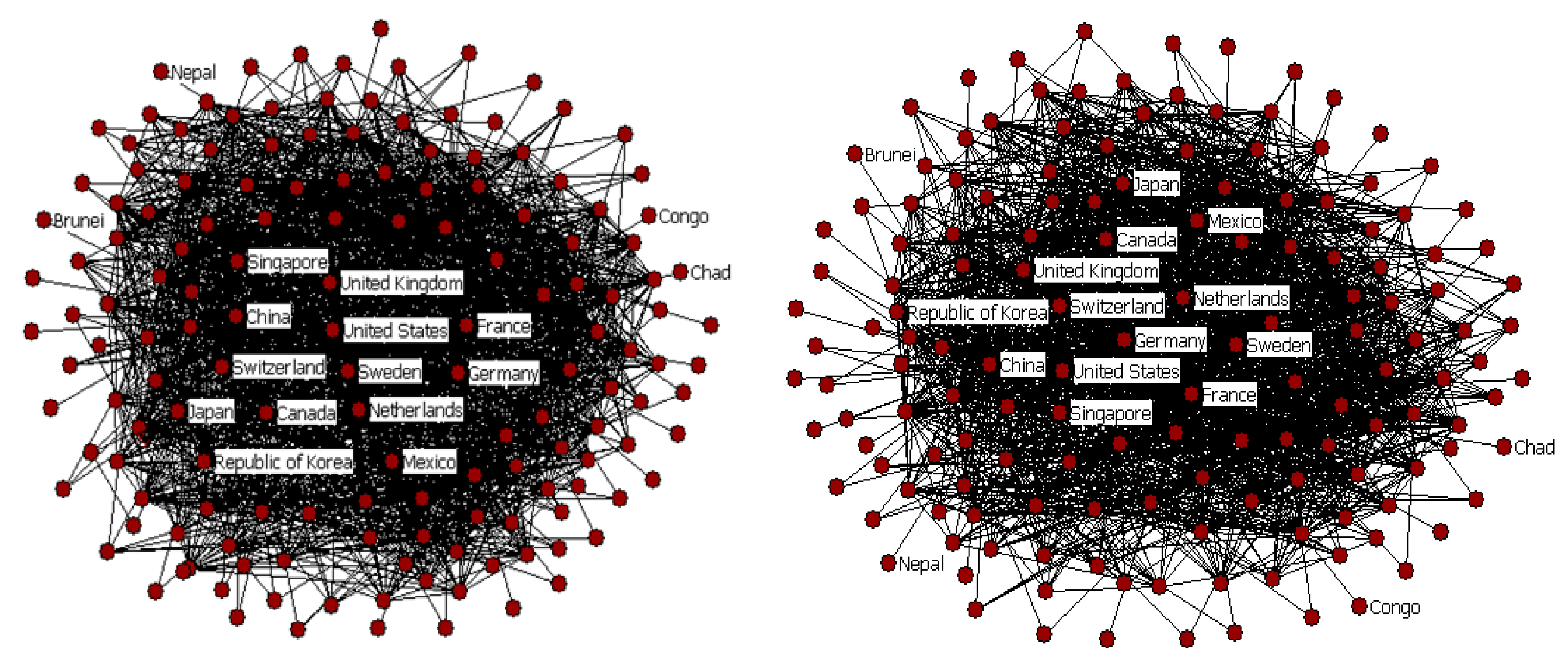
Figure 1 illustrates the bielemental networks for 2006/2010, and the nodes correspond to the 154 countries. In a bielemental network, the adjacency matrix between countries is symmetrical and the element in this adjacency matrix indicate whether country i and country j have an investment relationship. When there is investment relationship between countries, then the corresponding nodes are connected by a straight line. Otherwise there is no connection. Therefore, node linkages in a bielemental network are homogeneous. Figure 1 indicates that an international investment network is interlaced and spherical. Within the network, each country is highly interrelated and mutually reinforcing to affect network structure. Meanwhile, the spatial pattern of international direct investment is characterized by remarkable nonhomogeneity. There are close linkages between some countries and fewer linkages between others, which makes the node linkages of the entire network densely distributed in the middle area but sparsely on the periphery. Moreover, countries that are closely interrelated remain the centerpiece of this international investment network, such as the U.S., Germany, Switzerland, and France. The nodes representing China are gradually moving towards the center of network and maintain stronger investment linkages with the Netherlands, Singapore, the U.K. and the U.S. However, the ties that bind China and Japan as well as the Republic of Korea are loosening. Benefiting from the North America Free Trade Agreement, the investment positions of Canada and Mexico are significantly improved, and increases in Mexican outward investment into the other two countries are more obvious. Other countries, such as Chad, Nepal and the Congo, are located on the periphery of the network.

Figure 1. Binary network graph of international investment for 2006 and 2010.

Figure 1. Binary network graph of international investment for 2006 and 2010.

Considering that bielemental networks are concerned with investment linkages much more than investment direction or amount, directed weighted networks are further employed to analyze their topologies. In a directed weighted network, an investment relationship between countries can be expressed in a weighted adjacency matrix. The element in this matrix is the weight of one side in the network. It can be observed that a directed weighted network is a substantialized bielemental network. The average path length as well as the average clustering coefficient mainly reflects the global feature of the directed weighted network. Of the two, the former is the average distance between any two nodes, and the latter is probability of two nodes being directly connected with a given node. Moreover, the node degree and node strength reflect the bonds between two nodes. For the international investment network, the node degree is the number of countries that connect with a given node, while the node strength is the weight sum of all countries that connect with a given node. For a directed network, the node degree can be further divided into out-degree and in-degree categories. Specifically, the out-degree deals with the outbound links, in other words, the number of countries that become connected with a given country by investing overseas. The in-degree deals with the inbound links, in other words, the number of countries that become connected with a given country by introducing foreign funds. Similarly, out-strength indicates the sum of inflows to a country from investing overseas, while in-strength indicates the sum of inflows to a country from attracting foreign funds.

Table 1 lists some statistical indicators of the international investment network. It is clear that the average path length and average clustering coefficient remained at 2 and 0.5 respectively in recent years. That is, any two nodes have investment contact on two edges, and about half of countries maintain a direct investment connection with each other. Moreover, the average degree of the international investment network has remained at approximately 30 over the years, which indicates that each country is connected with 30 other countries on average. However, the average node strength increased at first and ultimately decreased. In 2007, the average strength of the international investment network peaked at 18,395.974 and then sharply declined because of the global banking crisis as well as the economic downturn, and it reached its lowest point of 7072.494 in 2010. The average out-strength and in-strength have followed the same trend.

Table 1. The structural characteristics of the international investment network between 2006 and 2010.

Year	2006	2007	2008	2009	2010
Number of connected edges	2302	2303	2302	2257	2251
Average path length	2.074	2.044	2.049	2.076	2.067
Average clustering coefficient	0.478	0.487	0.480	0.478	0.470
Average out-degree	14.948	14.955	14.948	14.656	14.617
Average in-degree	14.948	14.955	14.948	14.656	14.617
Average degree	29.896	29.910	29.896	29.312	29.234
Average out-strength	4912.310	9197.987	7610.671	5278.030	3536.247
Average in-strength	4912.310	9197.987	7610.671	5278.030	3536.247
Average strength	9824.620	18,395.974	15,221.342	10,556.060	7072.494

Table 1. The structural characteristics of the international investment network between 2006 and 2010.

Year	2006	2007	2008	2009	2010
Number of connected edges	2302	2303	2302	2257	2251
Average path length	2.074	2.044	2.049	2.076	2.067
Average clustering coefficient	0.478	0.487	0.480	0.478	0.470
Average out-degree	14.948	14.955	14.948	14.656	14.617
Average in-degree	14.948	14.955	14.948	14.656	14.617
Average degree	29.896	29.910	29.896	29.312	29.234
Average out-strength	4912.310	9197.987	7610.671	5278.030	3536.247
Average in-strength	4912.310	9197.987	7610.671	5278.030	3536.247
Average strength	9824.620	18,395.974	15,221.342	10,556.060	7072.494

In a complex network analysis, centrality is a structural indicator used to judge a node’s position and social prestige. Centrality can be assessed by degree centrality, closeness centrality and betweenness centrality. Degree centrality represents the capability of a country to connect with others and reveals whether this country is located in the center of the network group. Closeness centrality is a measurement of not being controlled by other nodes. In a network, if a node is close to other nodes, the distance between this node and other nodes is short and this node enjoys high closeness centrality. Therefore, the node has weak dependence on and is less controlled by others. Betweenness centrality measures the extent to which a node lies in the middle of other nodes; it is a control index. However, above centrality indexes are only used to measure binary networks. For this purpose, Random-Walk Betweenness Centrality, RWBC index for short, is put forward [20]. This indicator captures the effects of the magnitude of the relationship that a node has with other nodes as well as node strength in question. A higher RWBC index means that the related node is located at the center of the whole network.

Overall, countries with high centrality rankings are concentrated in the advanced economies of Western Europe and North America. Emerging economies such as China and Brazil have attempted to improve their node centrality. Table 2 lists the 10 countries with the highest average RWBC indexes between 2006 and 2010. It can be seen that the U.S., with the highest score, was at the core of the international investment network. As one of the world’s most open economies, the U.S. has consistently ranked first with the greatest capital inflow. Although its capacity in controlling the global investment network decreased slightly after the financial crisis in 2008, huge investment scale as well as economic strength maintained its core position. China was sub-central in the international investment network, and its RWBC index ranked in the top five over the years, ranking first in 2009. Moreover, according to analytical data of the RWBC index between 2006 and 2010, European and North American centrality declined after 2007, largely because the U.S. sub-loan crisis as well as the European debt crisis seriously affected foreign investment activities of developed countries, and the global economic recession compelled these countries to sharply reduce their investment. In the meantime, developing countries, such as China, Brazil and Argentina, played positive roles in this network. Compared with that of developed countries, developing countries sustained strong economic growth, which greatly increased investor confidence. We list the averages of three other centrality indexes. These centrality indexes demonstrate that the related indexes for China were obviously higher than those for other countries, mainly because some countries with negative net inflows were edited out and some countries that reported incomplete data were not absorbed into the samples, leading to fewer connected countries and affecting their status in the network. The analytical results further confirm that it is imperfect to use the node centrality calculated by the binary network to test a country’s position or its control capacity in the network.

Table 2. The 10 countries with the highest average RWBC indexes between 2006 and 2010.

Country	Degree centrality	Closeness centrality	Betweenness centrality	RWBC index
United States	66.869	65.513	9.935	143.277
China	68.235	69.546	15.034	112.446
UK	51.327	61.499	7.114	106.168
France	64.967	67.798	12.873	88.970
Canada	47.712	60.480	3.392	64.209
Brazil	56.863	63.048	8.535	47.176
Spain	34.641	55.312	2.884	36.892
Austria	38.562	57.286	3.152	25.184
Germany	54.379	63.110	5.426	24.333
Belgium	29.673	53.811	3.015	18.123

Table 2. The 10 countries with the highest average RWBC indexes between 2006 and 2010.

Country	Degree centrality	Closeness centrality	Betweenness centrality	RWBC index
United States	66.869	65.513	9.935	143.277
China	68.235	69.546	15.034	112.446
UK	51.327	61.499	7.114	106.168
France	64.967	67.798	12.873	88.970
Canada	47.712	60.480	3.392	64.209
Brazil	56.863	63.048	8.535	47.176
Spain	34.641	55.312	2.884	36.892
Austria	38.562	57.286	3.152	25.184
Germany	54.379	63.110	5.426	24.333
Belgium	29.673	53.811	3.015	18.123

With the continued expansion of the investment network and rapid development of bilateral business cooperation, global environmental pollution has become an increasingly serious problem. Global environmental pollution not only shows that regional pollution and ecological damage have worsened but also reflect that an environmental crisis is rapidly emerging. Among these environmental problems, the greenhouse effect and global warming caused by CO₂ emission have aroused public concern. Global CO₂ emissions increased from 20.537 billion tons in 1990 to 31.250 billion tons in 2010, and this acceleration was especially rapid in last ten years. The annual growth rate of CO₂ emissions is approximately 3%. Besides, the geographical distribution of environmental pollution demonstrates obvious clustering and inbalance in its characteristics. Moran’s Index for CO₂ emissions between 1990 and 2010 (the statistics of Moran’s Index are given in Table S1) is significantly positive, which suggests that the spatial distribution of CO₂ emissions has a remarkably positive autocorrelation (i.e., spatial dependency). In other words, the spatial distribution of environmental pollution is not random but tends to cluster in some countries. Heavily polluted countries tend to be neighbored by other heavily polluted ones, while lightly polluted countries tend to be neighbored by other lightly polluted ones. 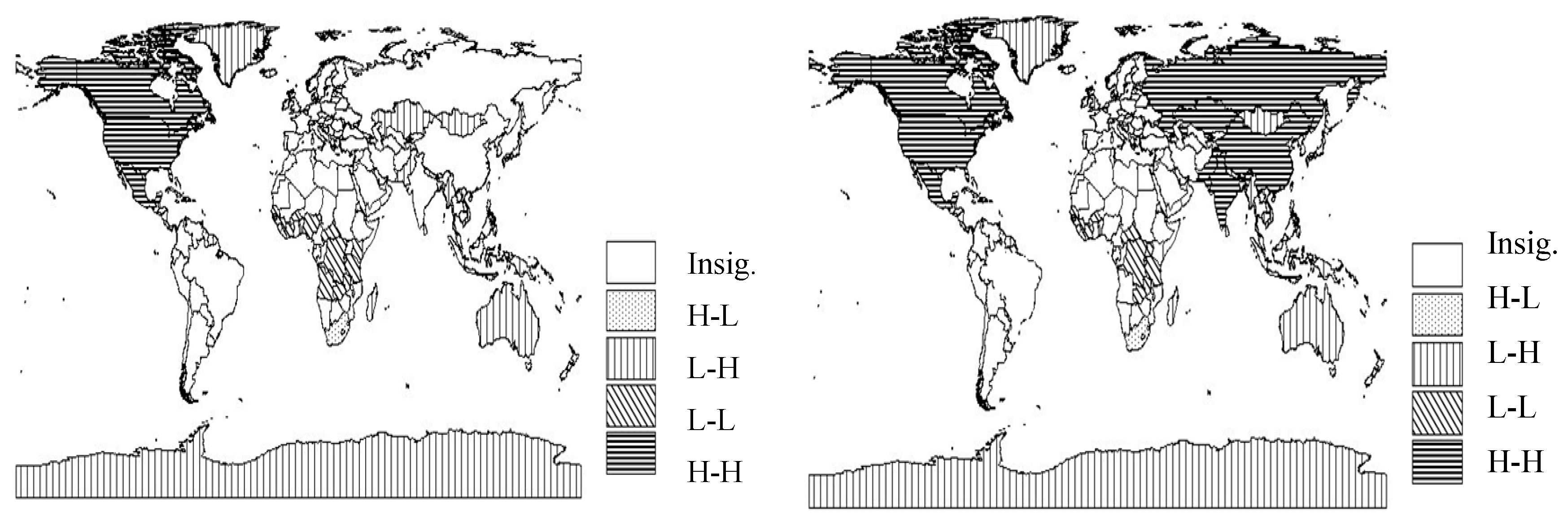Moreover, a scatter diagram of Moran’s Index is used to divide CO₂ clustering into four quadrants, namely, Quadrant I (H-H), Quadrant II (L-H), III (L-L) and Quadrant IV (H-L), and Local Indicators of Spatial Associations (LISA) cluster diagram is drawn to verify the resulting distribution pattern. The results indicate that Moran’s Index was above 0.12 before 2001, and the LISA scatter diagram shows high pollution clustering (i.e., H-H clustering) mainly occurred in North America and South Asia (as shown in Figure 2). However, after 2000, high pollution clustering began to expand to eastern and central Asia. In 2010, Moran’s Index of CO₂ emissions decreased to the minimum, and the LISA scatter diagram shows that North America, most Asian countries and Russia were surrounded by high pollution clustering, while low pollution clustering (i.e., L-L clustering) shrank dramatically across the globe, which indicates that environmental pressure worldwide increased.

Figure 2. Local Indicators of Spatial Associations (LISA) Clustering Map for CO₂ emissions in 2000 and 2010.

Figure 2. Local Indicators of Spatial Associations (LISA) Clustering Map for CO₂ emissions in 2000 and 2010.

3. Model Specification and Empirical Methodology

3.1. Model Specification

In order to examine how a country’s position in the international investment network affects environmental quality as well as the country’s role in transboundary pollution, we use the following equation.

$$P_{it}={\alpha }_0+{\alpha }_{1}Ln(pgd{p}_{it})+{\alpha }_{2}Ln{(pgd{p}_{it})}^2+{\alpha }_{3}Ln{(pgd{p}_{it})}^3+{\alpha }_{4}FNe{t}_{it}+{\alpha }_5{X}_{it}+{\epsilon }_{it}$$

(1)

The subscripts denote country i and time period t. P is indicator of environmental pollution, pgdp is GDP per capita, FNet is the index of the local investment network, and X denotes other control variables that affect pollution.

Considering that industrial transfers and policy externalities have served to strengthen the spatial association between environmental quality and economic growth [21], we establish spatial econometric models to reflect the spillover effects of environmental pollution. According to different forms of error shock on an observation’s spatial autocorrelation, spatial econometric models can be divided into the Spatial Error Model (SEM) and the Spatial Lag Model (SLM). The SEM assumes that spatial autocorrelation stems from the error shock of neighboring countries on the dependent variables, examining the effects of neighboring countries on local observation. Its econometric model can be expressed as:

$$P_{it}={\alpha }_0+{\alpha }_{1}Ln(pgd{p}_{it})+{\alpha }_{2}Ln{(pgd{p}_{it})}^2+{\alpha }_{3}Ln{(pgd{p}_{it})}^3+{\alpha }_{4}FNe{t}_{it}+{\alpha }_5{X}_{it}+{\epsilon }_{it}$$

Wherein

$${\epsilon }_i=\lambda {\displaystyle \sum _{j=1}^n{W}_{ij}}{\epsilon }_j+{\mu }_i {\mu }_i~N(0,{{\sigma }_i}^2)$$

(2)

In Equation (2), W_ij is the spatial weight matrix of size n × n. One assumption commonly encountered in the empirical literature is that the spatial weight matrix is based on the inverse geographical distances between countries’ centroids. λ is a scalar parameter to measure how the error shock of dependent variables in a neighborhood affects local observations.

The SLM assumes that spatial autocorrelation stems from dependent variables, examining the effects of environmental quality in neighboring countries on local pollution. Its econometric model can be expressed as

$$P_{it}=\rho {\displaystyle \sum _{j=1}^n{W}_{ij}}{P}_{jt}+{\alpha }_{1}Ln(pgd{p}_{it})+{\alpha }_{2}Ln{(pgd{p}_{it})}^2+{\alpha }_{3}Ln{(pgd{p}_{it})}^3+{\alpha }_{4}FNe{t}_{it}+{\alpha }_5{X}_{it}+{\epsilon }_{it}$$

(3)

The spatial regression coefficient ρ measures the effect of environmental pollution in neighboring countries on local pollution observations. ε is the vector for the random error term.

Moreover, the effects of international investment on environmental pollution depend on a country’s comparative advantage, which is driven by relative factor endowment and environmental regulation in the host country [22]. Based on Equations (2) and (3), we further incorporate the interaction term between the local network index and factor endowment advantage and that between the local network index and environmental regulation advantage to estimate the factor endowment effect and the pollution haven effect. The SEM can be then further expressed as

$$\begin{gathered} P_{it}={\alpha }_0+{\alpha }_{1}Ln(pgd{p}_{it})+{\alpha }_{2}Ln{(pgd{p}_{it})}^2+{\alpha }_{3}Ln{(pgd{p}_{it})}^3+{\alpha }_{4}FNe{t}_{it}+{\alpha }_{5}FNe{t}_{it}\times RK{L}_{it} \\ +{\alpha }_{6}FNe{t}_{it}\times RE{R}_{it}+{\alpha }_7{X}_{it}+{\epsilon }_{it}\prime \end{gathered}$$

Wherein

$${\epsilon }_i\prime =\lambda {\displaystyle \sum _{j=1}^n{W}_{ij}}{\epsilon }_j\prime +{\mu }_i\prime {\mu }_i\prime ~N(0,{\sigma }_i{\prime }^2)$$

(4)

The corresponding SLM can be expressed as

$$\begin{gathered} P_{it}=\rho {\displaystyle \sum _{j=1}^n{W}_{ij}}{P}_{jt}+{\alpha }_{1}Ln(pgd{p}_{it})+{\alpha }_{2}Ln{(pgd{p}_{it})}^2+{\alpha }_{3}Ln{(pgd{p}_{it})}^3+{\alpha }_{4}FNe{t}_{it}+{\alpha }_{5}FNe{t}_{it}\times RK{L}_{it} \\ +{\alpha }_{6}FNe{t}_{it}\times {RER}_{it}+{\alpha }_7{X}_{it}+{\epsilon }_{it}\prime \end{gathered}$$

(5)

RKL and RER indicate factor endowment advantage and environmental regulation advantage, respectively. FNet × RKL is the interaction term between the local network index and factor endowment advantage, and FNet × RER is the interaction term between the local network index and environmental regulation advantage. At the margin, the total effects of the local investment network on environmental pollution can be calculated by examining the following partial derivative:

$$\frac{\partial (P_{it})}{\partial (FNe{t}_{it})}={\alpha }_4+{\alpha }_{5}RK{L}_{it}+{\alpha }_{6}RE{R}_{it}$$

(6)

3.2. Variable Selection and Data Sources

For this paper, we have selected 154 countries with statistics between 2006 and 2010 as a sample. Bilateral direct investment data came from the International Trade Center database, CO₂ emission data came from the Carbon Dioxide Information Analysis Center, and other data with no special instructions came from the World Bank. Relevant variable indexing is as follows.

The dependent variable is environmental pollution (P). At present, pollutant concentrations and pollutant emissions are widely used to measure environmental pollution. Pollutant emissions reflect total discharge amount as a result of economic activities, while pollutant concentrations reflect emissions amount per unit area. Therefore, pollutant emissions are better suited to studying environmental effects, and pollutant concentrations are better suited to assessing welfare [23]. Given that this paper focuses on the impacts of international investment on global environmental quality, we choose CO₂ emissions, the main influence factor of environmental problems, to measure environmental pollution.

GDP per capita (pgdp) is an important variable that affects environmental pollution. The relationship between GDP per capita and environmental pollution may show an inverse U shape [24], or it might be represented by a rising, inverse U shape or a cubic shape depending on different countries and pollutants [25]. Hence, we use both the quadratic and cubic forms to describe the impact of output per capita on environmental pollution. The price factor is eliminated by the GDP deflator with a base year of 1990.

Local investment network (FNet) is our main independent variable. Previous studies mainly used actually utilized foreign capital to measure foreign investment [4]. This measurement cannot reflect investment relationships as well as investment destinations between countries. The boom of complex network analysis in recent decades offers beneficial references for the effective measurement of bilateral investment strength. Based on bilateral investment data between countries, we construct local network indexes, including node cohesion, node importance, and node centrality, to examine the role and position of a country in the international investment network. Specifically, we calculate the node cohesion of the local investment network using the node degree (including total degree, out-degree and in-degree) and node strength (including total strength, out-strength and in-strength) and examine the node centrality using degree centrality, closeness centrality, betweenness centrality, and the RWBC index.

The calculation of node importance is borrowed from Salancik [26], in which the node importance of country i can be expressed as

$$IM{P}_i={\displaystyle \sum DE{P}_{ij}}\cdot IM{P}_j+I{V}_i$$

(7)

Wherein IMP_i is the index of the node importance of country i. DEP_ij indicates the dependency of country j on the investment of country i, and it is measured in two aspects, namely, the dependency of the capital-outflow country (calculated by the proportion of the investment of country j in country i in the total external investment of country j) and the dependency of the capital-recipient country (calculated by the proportion of investment of country i in country j in the total foreign capital utilized by country j). IV_i denotes the intrinsic value of country i and considers three alternatives: (1) It is set constant (IV = 1) essentially because precisely measuring the extent to which one node is more important than another is very difficult; (2) Considering a country’s capability to participate in international investment, we use the share of investment inflows of country i in the total amount of global investment to denote its intrinsic value (IV = IS); and (3) The ratio of GDP per capita of country i with respect to that of the U.S. is used to denote its intrinsic value (IV = RU). Thus, nodes are considered more important when other nodes depend more on them and when the other nodes depending on them are themselves important.

To minimize estimation bias due to omitted variables, we add another control variable X that affects pollution. The following variables are included.

Trade openness (Openness). More openness to trade exacerbates resource consumption and pollutant emissions while promoting economic growth. Moreover, it produces profound influences on the environment through a green trade barrier, cleaner technology spillovers, pollution transfers, etc. [27]. As a measure of trade openness, we use the share of total trade (exports plus imports) within the GDP of a country.

Capital-labor ratio (K/L). Generally speaking, capital-intensive industries are likely to produce more pollutant emissions and to worsen environmental quality [16]. The amount of capital inventory is estimated by the perpetual inventory method used by Leamer [28], the depreciation rate is set at 7 percent, and the price factor is eliminated by using the GDP deflator.

Energy efficiency (Energy). The improvement of energy efficiency is beneficial to reducing pollution, and this index is measured by the ratio of GDP to energy consumption.

Industrial structure (Manufacturing). Quickening industrialization means the unrestrained exploitation of natural resources and a sharp increase in waste emissions, and higher industrial added value brings more pollutants [29]. Industrial structure is measured by the ratio of industrial added value in manufacturing to GDP.

Population density (Population). High population density will produce more pollution on the one hand and increase the input of environmental participants to protect the local environment on the other hand. Hence, population density is an important factor that impacts environmental pollution as well. It is measured by the number of people per unit area.

Environmental regulation (ER). As incomes rise, people attach increasing importance to environmental quality, and governments make every effort to protect ecological environment. We use the number of international environmental agreements (IEAs) to measure environmental regulation in each country, which is frequently used in the literature [30,31]. These international environmental agreements include the Ramsar Convention, Vienna Convention, the United Nations Framework on the Convention for Climate Change, the Kyoto Protocol, the Stockholm Convention on Persistent Organic Pollutants, the Convention on Biological Diversity and the Convention on Migratory species. If a country signs one of these international environmental agreements, its score for environmental regulation is 1; otherwise, its score is 0. The final environmental regulation is the total score for the above agreements.

Moreover, there are certain limitations in the current literature on measuring factor endowment, such as weaknesses in data collection for factor inputs and inconsistent criteria for factor endowments. Antweiler et al. [23] used the ratio of a country’s capital-labor ratio to the world average, which is widely used in other scholars’ research, such as Cole et al. [32], Zhou and Zhu [33]. Therefore, this measurement is also referential to our research. If this ratio is larger than 1, then country i has an obvious factor endowment advantage. Meanwhile, environmental regulation advantage is measured by the ratio of environmental regulation in country i to the world average.

Given that the values of in-degree, in-strength and node centrality in individual countries are 0, the indexes of the local investment network measured by node cohesion and node centrality are assessed by initial data in the regression, and other variables are defined by natural logarithms. An overview of the descriptive statistics of these data is provided in Table S2.

3.3. Empirical Methodology

The maximum likelihood (ML) estimation procedure is used for the estimation of the parameters of both the SEM and the SLM [18]. This method not only overcomes the problem of variable endogeneity that exists in traditional OLS but also identifies the real source of spatial features in the models by comparing the value of likelihood.

4. Empirical Results

The estimated results in Table 3 indicate that the value of Moran is positive and rejects the null hypothesis at 1 percent significance. Therefore, spatial correlation is incorporated into our analysis. In terms of the model judgment criteria used by Anselin et al. [18], we find that the statistic of Lmerr is more significant than that of Lmlag, and the Robust-Lmerr statistic is more significant than that of Robust-Lmlag. Hausman test shows that fixed effects are stronger than random effects, and in some specific individual analyses, the fixed effect model is a better choice [34]; thus the fixed effects of the SEM are more suitable to conduct regressions. Our regression results are presented in Table 3.

Table 3. Estimated Results of SEM for Node Cohesion on CO₂ emissions.

	Result 1	Result 2	Result 3	Result 4	Result 5	Result 6
pgdp (GDP per capita)	−0.214	3.576 *	−4.972 **	−5.086 **	−5.686 **	−5.424 **
	(−0.095)	(1.682)	(−2.023)	(−2.102)	(−2.316)	(−2.194)
pgdp2	0.161	−0.220	0.730 **	0.821 ***	0.898 ***	0.842 ***
	(0.571)	(−0.827)	(2.360)	(2.699)	(2.910)	(2.709)
pgdp3	−0.012	−0.001	−0.033 ***	−0.040 ***	−0.043 ***	−0.040 ***
	(−1.010)	(−0.072)	(−2.589)	(−3.226)	(−3.420)	(−3.149)
FNet(Node)	0.039 ***			0.158***
	(17.130)			(10.223)
FNet(Out)		0.092 ***			0.249 ***
		(20.618)			(8.835)
FNet(In)			0.032 ***			0.213 ***
			(9.514)			(8.315)
Openness	−0.454 ***	−0.621 ***	−0.637 ***	−0.748 ***	−0.812 ***	−0.777 ***
	(−4.058)	(−6.016)	(−5.120)	(−6.213)	(−6.671)	(−6.322)
K/L (Capital-labor ratio)	0.082 **	0.058 *	0.177 ***	0.176 ***	0.182 ***	0.206 ***
	(2.234)	(1.671)	(4.428)	(4.489)	(4.575)	(5.186)
Energy	−0.364 ***	−0.313 ***	−0.448 ***	−0.440 ***	−0.442 ***	−0.464 ***
	(−9.963)	(−9.029)	(−11.199)	(−11.125)	(−10.990)	(−11.530)
Manufacturing	1.104 ***	1.301 ***	1.053 ***	1.155 ***	1.171 ***	1.132 ***
	(9.599)	(12.045)	(8.213)	(9.179)	(9.157)	(8.804)
Population	0.140 ***	0.120 ***	0.144 ***	0.158 ***	0.118 ***	0.180 ***
	(3.495)	(3.199)	(3.234)	(3.588)	(2.636)	(3.977)
ER (Environmental regulation)	0.125	0.083	0.530 ***	0.709 ***	0.789 ***	0.724 ***
	(0.678)	(0.479)	(2.628)	(3.591)	(3.943)	(3.587)
λ	0.465 ***	0.533 ***	0.468 ***	0.548 ***	0.542 ***	0.531 ***
	(6.515)	(8.260)	(6.584)	(8.703)	(8.522)	(8.202)
R2	0.629	0.672	0.541	0.552	0.538	0.532
Log L	−1402.214	−1356.795	−1483.691	−1477.079	−1488.905	−1492.933
Moran	8.490 ***	11.304 ***	7.881 ***	10.634 ***	10.629 ***	9.852 ***

Note: The values in brackets are the t-statistics of corresponding estimated coefficients, and ***, ** and * denote significance at 1%, 5% and 10%, respectively. These conditions remain the same in the following tables.

Table 3. Estimated Results of SEM for Node Cohesion on CO₂ emissions.

	Result 1	Result 2	Result 3	Result 4	Result 5	Result 6
pgdp (GDP per capita)	−0.214	3.576 *	−4.972 **	−5.086 **	−5.686 **	−5.424 **
	(−0.095)	(1.682)	(−2.023)	(−2.102)	(−2.316)	(−2.194)
pgdp2	0.161	−0.220	0.730 **	0.821 ***	0.898 ***	0.842 ***
	(0.571)	(−0.827)	(2.360)	(2.699)	(2.910)	(2.709)
pgdp3	−0.012	−0.001	−0.033 ***	−0.040 ***	−0.043 ***	−0.040 ***
	(−1.010)	(−0.072)	(−2.589)	(−3.226)	(−3.420)	(−3.149)
FNet(Node)	0.039 ***			0.158***
	(17.130)			(10.223)
FNet(Out)		0.092 ***			0.249 ***
		(20.618)			(8.835)
FNet(In)			0.032 ***			0.213 ***
			(9.514)			(8.315)
Openness	−0.454 ***	−0.621 ***	−0.637 ***	−0.748 ***	−0.812 ***	−0.777 ***
	(−4.058)	(−6.016)	(−5.120)	(−6.213)	(−6.671)	(−6.322)
K/L (Capital-labor ratio)	0.082 **	0.058 *	0.177 ***	0.176 ***	0.182 ***	0.206 ***
	(2.234)	(1.671)	(4.428)	(4.489)	(4.575)	(5.186)
Energy	−0.364 ***	−0.313 ***	−0.448 ***	−0.440 ***	−0.442 ***	−0.464 ***
	(−9.963)	(−9.029)	(−11.199)	(−11.125)	(−10.990)	(−11.530)
Manufacturing	1.104 ***	1.301 ***	1.053 ***	1.155 ***	1.171 ***	1.132 ***
	(9.599)	(12.045)	(8.213)	(9.179)	(9.157)	(8.804)
Population	0.140 ***	0.120 ***	0.144 ***	0.158 ***	0.118 ***	0.180 ***
	(3.495)	(3.199)	(3.234)	(3.588)	(2.636)	(3.977)
ER (Environmental regulation)	0.125	0.083	0.530 ***	0.709 ***	0.789 ***	0.724 ***
	(0.678)	(0.479)	(2.628)	(3.591)	(3.943)	(3.587)
λ	0.465 ***	0.533 ***	0.468 ***	0.548 ***	0.542 ***	0.531 ***
	(6.515)	(8.260)	(6.584)	(8.703)	(8.522)	(8.202)
R2	0.629	0.672	0.541	0.552	0.538	0.532
Log L	−1402.214	−1356.795	−1483.691	−1477.079	−1488.905	−1492.933
Moran	8.490 ***	11.304 ***	7.881 ***	10.634 ***	10.629 ***	9.852 ***

Note: The values in brackets are the t-statistics of corresponding estimated coefficients, and ***, ** and * denote significance at 1%, 5% and 10%, respectively. These conditions remain the same in the following tables.

Results 1 to 3 in Table 3 correspond to the information obtained when total degree, in-degree and out-degree are used, respectively, to measure the local investment network in the analysis of the relationship between node degree and CO₂ emissions, while Results 4 to 6 show the estimates when total strength, in-strength and out-strength are used, respectively, to measure the local investment network in the analysis. According to the estimated results in Table 3, λ is significantly positive, so environmental pollution has strong spillover effects, and this conclusion is consistent with the empirical research of Maddison [21].

The key result in Table 3 is that the tight connection between nodes significantly impact global environmental pollution. Specifically, Result 1 reveals that a unit increase in the total degree of a given node increases CO₂ emissions by 0.039% on average, while Result 4 reveals that a unit increase in the total strength increases CO₂ emissions by 0.158%. Possibly, countries enlarge mutual investment to construct a complex network. The network not only expands the production scale as the number of investment partners increases but also affects the global environment through direct and hidden drainage channels. This conclusion is consistent with that described in Millimet and List [35]. Moreover, Result 2 and Result 3 suggest that out-degree has a greater negative effect on environmental quality than in-degree, whereas Result 5 and Result 6 suggest that out-strength has a stronger effect on environment than in-strength. The main reason is that most out-degree(or out-strength) is obviously higher than corresponding in-degree (or in-strength).When overseas investment worsens environmental quality in the host country, it indubitably sends a negative environmental signal to other countries around this network, thereby stimulating dirty products and finally affecting the environment in the home country.

We further test the impacts of node cohesion in developed and developing countries (shown in Table 4). The test results reveal that both out-degree and out-strength in developing countries have greater negative effects on environmental quality than they do in developed countries, and we proffer an explanation of how and why this happens. At present, most developing countries are at the lower end of global value chain, and their investment destinations are concentrated in other poorer countries. This global specialization and overseas investment will stimulate the export-led growth of raw materials and intermediate products in home country, creating resource consumption and environmental pollution. Moreover, some investment from developing countries flows into developed countries that enjoy higher economic development. However, if their technological progress and structural adjustment obtained through an open “Going-out” strategy are not linked to conserving energy and reducing emissions, these reverse technology spillover and structural optimization effects would threaten sustainable development of overseas investment. The conclusion is in line with Zhou and Pang [36]. In contrast, overseas investment of developed countries can make their industrial structure favor labor-intensive products. They can also use their dominance over the worldwide production network to transfer obsolete energy-consumption and heavy-pollution industries to developing countries. In such a way, their investment has a smaller negative impact on domestic environment.

In addition, Result 11 and Result 12 in Table 4 demonstrate that the improvement of in-strength will remarkably deteriorate the host environment, but this side effect is more devastating than that in developed countries. It may be that developing countries absorb approximately 60% of the international funds in our sample period, and these funds are mainly in the manufacturing sector with lower technology, their production increases pollutant emissions. This means that developing countries will not only maintain high vigilance to the inflows of pollution-intensive FDI but also pay close attention to indirect pollution effects. Compared with developing countries, the service industries of developed countries occupy predominant positions in absorbing foreign capital, and they produce less pollution than other industries, so the utilization of FDI in developed countries has a smaller impact on the host environment. This conclusion is in line with Wood [37].

Table 4. Estimated results of node cohesion on CO₂ emissions in different countries.

	Node degree		Out-degree		In-degree		Node strength		Out-strength		In-strength
	Result 1	Result 2	Result 3	Result 4	Result 5	Result 6	Result 7	Result 8	Result 9	Result 10	Result 11	Result 12
pgdp	−6.710 ***	−6.617 ***	−6.230 ***	−1.469	−6.634 **	−5.272 **	−6.541 **	−5.362 **	−9.698 ***	−5.822 **	−9.712 ***	−9.605 ***
	(−2.601)	(−2.563)	(−2.421)	(−0.631)	(−2.576)	(−2.125)	(−2.554)	(−2.187)	(−3.546)	(−2.347)	(−3.552)	(−3.511)
pgdp2	0.987 ***	0.976 ***	0.931 ***	0.370	0.977 ***	0.775 **	0.970 ***	0.848 ***	1.342 ***	0.908 ***	1.344 ***	1.330 ***
	(3.043)	(3.006)	(2.879)	(1.266)	(3.017)	(2.483)	(3.013)	(2.752)	(3.911)	(2.911)	(3.919)	(3.876)
pgdp3	−0.045 ***	−0.044 ***	−0.043 ***	−0.022 *	−0.044 ***	−0.035 ***	−0.044 ***	−0.041 ***	−0.059 ***	−0.043 ***	−0.059 ***	−0.058 ***
	(−3.379)	(−3.345)	(−3.237)	(−1.868)	(−3.352)	(−2.733)	(−3.370)	(−3.240)	(−4.169)	(−3.385)	(−4.178)	(−4.134)
FNet	0.001						0.011 ***
(Node-developed)	(0.337)						(3.237)
FNet		0.006						0.149 ***
(Node-developing)		(0.330)						(9.041)
FNet			0.018 **						0.140 **
			(2.503)						(2.285)
(Out-developed)
FNet				0.061 ***						0.242 ***
										(7.814)
				(14.176)
(Out-developing)
FNet					0.014 *						0.185 ***
											(2.717)
(In-developed)					(1.783)
FNet						0.029 ***						0.216 **
(In-developing)						(8.437)						(2.311)
Control variables	yes	yes	yes	yes	yes	yes	yes	yes	yes	yes	yes	yes
λ	0.522 ***	0.527 ***	0.524 ***	0.511 ***	0.523 ***	0.486 ***	0.524 ***	0.543 ***	0.554 **	0.540 ***	0.425 ***	0.454 ***
	(7.949)	(8.089)	(8.005)	(7.652)	(7.977)	(7.013)	(8.005)	(8.553)	(8.580)	(8.462)	(5.592)	(6.592)
R2	0.490	0.490	0.494	0.595	0.491	0.531	0.497	0.540	0.498	0.528	0.438	0.437
Log L	−1525.995	−1525.989	−1522.929	−1436.806	−1524.952	−1492.231	−1520.846	−1487.218	−1507.131	−1495.773	−1556.981	−1557.603
Moran	9.644 ***	9.669 ***	9.681 ***	9.883 ***	9.525 ***	8.287 ***	9.636 ***	10.447 ***	6.825 ***	10.582 ***	6.832 ***	6.824 ***

Note: (1) FNet (out-developed) indicates the out-degree (or corresponding out-strength) in developed countries. FNet (out-developing) indicates the out-degree (or corresponding out-strength) in developing countries; (2) FNet (in-developed) indicates the in-degree (or corresponding in-strength) in developed countries. FNet (in-developing) indicates the in-degree (or corresponding in-strength) in developing countries.

Table 4. Estimated results of node cohesion on CO₂ emissions in different countries.

	Node degree		Out-degree		In-degree		Node strength		Out-strength		In-strength
	Result 1	Result 2	Result 3	Result 4	Result 5	Result 6	Result 7	Result 8	Result 9	Result 10	Result 11	Result 12
pgdp	−6.710 ***	−6.617 ***	−6.230 ***	−1.469	−6.634 **	−5.272 **	−6.541 **	−5.362 **	−9.698 ***	−5.822 **	−9.712 ***	−9.605 ***
	(−2.601)	(−2.563)	(−2.421)	(−0.631)	(−2.576)	(−2.125)	(−2.554)	(−2.187)	(−3.546)	(−2.347)	(−3.552)	(−3.511)
pgdp2	0.987 ***	0.976 ***	0.931 ***	0.370	0.977 ***	0.775 **	0.970 ***	0.848 ***	1.342 ***	0.908 ***	1.344 ***	1.330 ***
	(3.043)	(3.006)	(2.879)	(1.266)	(3.017)	(2.483)	(3.013)	(2.752)	(3.911)	(2.911)	(3.919)	(3.876)
pgdp3	−0.045 ***	−0.044 ***	−0.043 ***	−0.022 *	−0.044 ***	−0.035 ***	−0.044 ***	−0.041 ***	−0.059 ***	−0.043 ***	−0.059 ***	−0.058 ***
	(−3.379)	(−3.345)	(−3.237)	(−1.868)	(−3.352)	(−2.733)	(−3.370)	(−3.240)	(−4.169)	(−3.385)	(−4.178)	(−4.134)
FNet	0.001						0.011 ***
(Node-developed)	(0.337)						(3.237)
FNet		0.006						0.149 ***
(Node-developing)		(0.330)						(9.041)
FNet			0.018 **						0.140 **
			(2.503)						(2.285)
(Out-developed)
FNet				0.061 ***						0.242 ***
										(7.814)
				(14.176)
(Out-developing)
FNet					0.014 *						0.185 ***
											(2.717)
(In-developed)					(1.783)
FNet						0.029 ***						0.216 **
(In-developing)						(8.437)						(2.311)
Control variables	yes	yes	yes	yes	yes	yes	yes	yes	yes	yes	yes	yes
λ	0.522 ***	0.527 ***	0.524 ***	0.511 ***	0.523 ***	0.486 ***	0.524 ***	0.543 ***	0.554 **	0.540 ***	0.425 ***	0.454 ***
	(7.949)	(8.089)	(8.005)	(7.652)	(7.977)	(7.013)	(8.005)	(8.553)	(8.580)	(8.462)	(5.592)	(6.592)
R2	0.490	0.490	0.494	0.595	0.491	0.531	0.497	0.540	0.498	0.528	0.438	0.437
Log L	−1525.995	−1525.989	−1522.929	−1436.806	−1524.952	−1492.231	−1520.846	−1487.218	−1507.131	−1495.773	−1556.981	−1557.603
Moran	9.644 ***	9.669 ***	9.681 ***	9.883 ***	9.525 ***	8.287 ***	9.636 ***	10.447 ***	6.825 ***	10.582 ***	6.832 ***	6.824 ***

Note: (1) FNet (out-developed) indicates the out-degree (or corresponding out-strength) in developed countries. FNet (out-developing) indicates the out-degree (or corresponding out-strength) in developing countries; (2) FNet (in-developed) indicates the in-degree (or corresponding in-strength) in developed countries. FNet (in-developing) indicates the in-degree (or corresponding in-strength) in developing countries.

In Table 5, Results 1 to 3 examine how the node importance affects global environmental quality from the perspective of capital outflows , and Results 4 to 6 study the extent to which a country’s importance affects global CO₂ emissions from the perspective of capital inflows. Results 7 to 10 test the influence of a country’s centrality on the environment based on different network centrality indexes. The estimated results in Table 5 show that the coefficients of node importance and node centrality are significantly positive, indicating that the improvements of node importance as well as its centrality will exacerbate environmental problems. For example, it can be seen from Result 2 and Result 10 that a 1% increase in node importance increases CO₂ emissions by 0.114%, and that a unit increase in node centrality increases CO₂ emissions by 0.031%. Thus, network structure remarkably affects regional environment, and it appears the higher the node importance and node centrality are, the more dependence and control the corresponding country has. Under these circumstances, the speed of polluting transfers in this network is faster, and the effects of transboundary pollution are stronger.

The empirical results in Table 5 also show that the estimated coefficients of node importance in capital-outflow countries are significantly lower than those of node importance in capital-recipient countries. Results 1 to 3 demonstrate that the node importance of capital-outflow countries improves 1%, and CO₂ emissions increase 0.083%–0.114%. Results 4 to 6 show that the node importance of capital-recipient countries improves 1%, and CO₂ emissions increase 0.104%–0.343%. One possible reason for these results is that capital-recipient countries with higher node importance have greater dependence on international investment. In order to attract more foreign funds or consolidate existing FDI, local governments have enough incentives to outperform the competition for foreign investment by undertaking initiatives to reduce environmental standards (i.e., the “race to the bottom”), which has been supported by Benarroch and Thille [38].Capital-outflow countries with higher node importance optimize the use of close investment linkages to transfer high-polluting industries to other areas. Hence, their overseas investment has a minor side effect on the domestic environment.

Table 5. Estimated results for the effects of node importance and node centrality on CO₂ emission.

	Node importance						Node centrality
	Result 1	Result 2	Result 3	Result 4	Result 5	Result 6	Result 7	Result 8	Result 9	Result 10
pgdp	−5.021 **	−4.957 **	−6.018 **	−5.489 **	−5.537 **	−6.968 ***	−0.171	−4.500*	−5.353 ***	−5.478 ***
	(−1.985)	(−2.030)	(−2.376)	(−2.135)	(−2.283)	(−2.712)	(−0.078)	(−1.835)	(−2.231)	(−2.274)
pgdp2	0.766 **	0.747 **	0.883 ***	0.831 **	0.819 ***	1.006 ***	0.158	0.707 **	0.804 ***	0.835 ***
	(2.407)	(2.432)	(2.771)	(2.570)	(2.686)	(3.115)	(0.564)	(2.294)	(2.665)	(2.758)
pgdp3	−0.035 ***	−0.034 ***	−0.040 ***	−0.038 ***	−0.037 ***	−0.045 ***	−0.012	−0.034 ***	−0.037 ***	−0.039 ***
	(−2.719)	(−2.714)	(−3.076)	(−2.894)	(−2.960)	(−3.433)	(−1.002)	(−2.675)	(−3.012)	(−3.178)
Importance	0.104 ***			0.343 ***
(IV = 1)	(6.452)			(4.186)
Importance		0.114 ***			0.200 ***
(IV = IS)		(10.055)			(10.908)
Importance			0.083 ***			0.104 ***
(IV = RU)
			(5.716)			(2.888)
Centrality							0.076 ***
(DC)
							(17.408)
Centrality								0.055 ***
(CC)								(9.199)
Centrality									0.299 ***
(BC)									(11.205)
Centrality										0.031 ***
(RWBC)										(10.734)
Control variables	yes	yes	yes	yes	yes	yes	yes	yes	yes	yes
λ	0.502 ***	0.467 ***	0.510 ***	0.499 ***	0.410 ***	0.510 ***	0.445 ***	0.557 ***	0.497 ***	0.520 ***
	(7.415)	(6.561)	(7.389)	(7.364)	(5.352)	(7.390)	(6.071)	(8.982)	(7.287)	(7.893)
R2	0.515	0.547	0.510	0.500	0.553	0.494	0.631	0.542	0.560	0.556
Log L	−1505.867	−1478.996	−1510.145	−1517.487	−1472.294	−1521.995	−1398.810	−1485.982	−1468.021	−1472.375
Moran	9.355 ***	8.118 ***	9.033 ***	8.588 ***	5.036 ***	8.809 ***	7.970 ***	14.944 ***	8.950 ***	9.846 ***

Note: (1) In Table 5, the indexes of node importance in Results 1 to 3 are calculated by the investment dependence of capital-outflow countries; the indexes of node importance in Results 4 to 6 are calculated by the investment dependence of capital-recipient countries; and the indexes of node centrality in Results 7 to 10 are calculated by degree centrality, closeness centrality, betweenness centrality and RWBC index. (2) Importance (IV = 1) indicates that the node importance is calculated in terms of property value as 1; Importance (IV=IS) indicates that the node importance is calculated by its property value, equaling the share of investment inflows of a country out of total world investment to denote its intrinsic value; Importance (IV=RU) indicates that the node importance is calculated by its property value, equaling the ratio of the GDP per capita of a country with respect to that of the U.S.

Table 5. Estimated results for the effects of node importance and node centrality on CO₂ emission.

	Node importance						Node centrality
	Result 1	Result 2	Result 3	Result 4	Result 5	Result 6	Result 7	Result 8	Result 9	Result 10
pgdp	−5.021 **	−4.957 **	−6.018 **	−5.489 **	−5.537 **	−6.968 ***	−0.171	−4.500*	−5.353 ***	−5.478 ***
	(−1.985)	(−2.030)	(−2.376)	(−2.135)	(−2.283)	(−2.712)	(−0.078)	(−1.835)	(−2.231)	(−2.274)
pgdp2	0.766 **	0.747 **	0.883 ***	0.831 **	0.819 ***	1.006 ***	0.158	0.707 **	0.804 ***	0.835 ***
	(2.407)	(2.432)	(2.771)	(2.570)	(2.686)	(3.115)	(0.564)	(2.294)	(2.665)	(2.758)
pgdp3	−0.035 ***	−0.034 ***	−0.040 ***	−0.038 ***	−0.037 ***	−0.045 ***	−0.012	−0.034 ***	−0.037 ***	−0.039 ***
	(−2.719)	(−2.714)	(−3.076)	(−2.894)	(−2.960)	(−3.433)	(−1.002)	(−2.675)	(−3.012)	(−3.178)
Importance	0.104 ***			0.343 ***
(IV = 1)	(6.452)			(4.186)
Importance		0.114 ***			0.200 ***
(IV = IS)		(10.055)			(10.908)
Importance			0.083 ***			0.104 ***
(IV = RU)
			(5.716)			(2.888)
Centrality							0.076 ***
(DC)
							(17.408)
Centrality								0.055 ***
(CC)								(9.199)
Centrality									0.299 ***
(BC)									(11.205)
Centrality										0.031 ***
(RWBC)										(10.734)
Control variables	yes	yes	yes	yes	yes	yes	yes	yes	yes	yes
λ	0.502 ***	0.467 ***	0.510 ***	0.499 ***	0.410 ***	0.510 ***	0.445 ***	0.557 ***	0.497 ***	0.520 ***
	(7.415)	(6.561)	(7.389)	(7.364)	(5.352)	(7.390)	(6.071)	(8.982)	(7.287)	(7.893)
R2	0.515	0.547	0.510	0.500	0.553	0.494	0.631	0.542	0.560	0.556
Log L	−1505.867	−1478.996	−1510.145	−1517.487	−1472.294	−1521.995	−1398.810	−1485.982	−1468.021	−1472.375
Moran	9.355 ***	8.118 ***	9.033 ***	8.588 ***	5.036 ***	8.809 ***	7.970 ***	14.944 ***	8.950 ***	9.846 ***

Note: (1) In Table 5, the indexes of node importance in Results 1 to 3 are calculated by the investment dependence of capital-outflow countries; the indexes of node importance in Results 4 to 6 are calculated by the investment dependence of capital-recipient countries; and the indexes of node centrality in Results 7 to 10 are calculated by degree centrality, closeness centrality, betweenness centrality and RWBC index. (2) Importance (IV = 1) indicates that the node importance is calculated in terms of property value as 1; Importance (IV=IS) indicates that the node importance is calculated by its property value, equaling the share of investment inflows of a country out of total world investment to denote its intrinsic value; Importance (IV=RU) indicates that the node importance is calculated by its property value, equaling the ratio of the GDP per capita of a country with respect to that of the U.S.

We further examine the effects of node importance and node centrality on the environmental quality of the host country from the perspective of capital-outflow countries (empirical results are shown in Table S3). The estimated results for node importance show that the estimated coefficients of local investment network in developing countries are obviously higher than that in developed countries. Specifically, the node importance of developing countries rises 1%, and CO₂ emissions in host countries increase 0.083%–0.108% on average, which is 0.056%–0.094% higher than that of developed countries. An explanation for this result could be that developing countries’ high dependency makes them become more easily involved in a captive network, and induces their overseas investment to concentrate on polluting industries. China is a typical case, as over 75% of its overseas mergers and acquisitions concentrate in energy and mineral resource fields. Hence they pollute the host environment heavily and eventually cause green barriers in the long run. Some developed countries can make full use of their high node dependency to strengthen investment bonds with others, especially subsidiaries in host countries. Through these subsidiaries, they may evade their environmental responsibility in local area.

Moreover, node centrality of developed countries improves a one-unit, and CO₂ emissions increase 0.016%–0.314%. These estimated coefficients are obviously higher than those of developing countries, so the improvement of the node status in developed countries brings greater environmental pollution to host areas. Presumably, developed countries use their higher dependency and core positions in the international investment network to undertaking rent-seeking activities on a global scale and transfer polluting industries to other countries, particularly developing countries with higher node dependency. In such a case, multinationals located in the center of a network will use developing countries to take on value chain linkages with high-energy consumption and pollution, thereby causing host countries to bear high pollution. In contrast, the superior node centrality of developing countries will undoubtedly enhance their control capacity over key resources in the global production network, and technical requirements in the supply chain and value-added chain will improve accordingly. Thus, their investment has a minor side effect on the host environment. The above estimated results further validate the rationality of the results presented in Table 4.

Table 6 lists the estimated results for the factor endowment effect and the pollution haven effect caused by the international investment network. The coefficients of the interaction terms between the local network index and factor endowment advantage are almost significantly positive. It means that the international investment network makes countries that have obvious capital advantage more likely specialize in pollution-intensive products, and the international investment network on the basis of factor advantage increases this pollution. As shown in Result 2 and Result 3, the estimated coefficients of the interaction terms between in-degree and factor endowment advantage are remarkably higher than those for out-degree. Combining with Result 6, one explanation is that the inflows of foreign funds further increase capital abundance in a country where it has obvious capital advantage. This can lead to the country being locked in capital-intensive production with high pollution. Capital-outflow countries can use close investment linkages to transfer their pollution-intensive industries through this network; thus, they have reduced side effects on the environment. Moreover, the empirical results also indicate that the coefficient of interaction terms (Importance × RKL) in capital-recipient countries is obviously higher than that for capital-outflow countries. Higher node importance may incentivize capital-recipient countries, which have obvious advantage of factor endowment, to specialize in pollution-intensive products, and provide pollution transfer channels to capital-outflow countries. It is worthwhile to note that the coefficient of interaction terms between node importance and the factor endowment advantage in Result 9 is positive but fails to pass a 10 percent significance test. A possible explanation may be that node importance, which is calculated based on the share of investment inflows, reinforces the influence of its capital flows on other nodes. Countries that enjoy higher node dependency can more easily transfer its polluting industries or capital to change existing advantage, thus reducing pollutant emissions. This statement is in line with Kali and Reyes [39]. Besides, increasing the node centrality calculated with four different indexes by 1 unit is associated with an average increase of CO₂ emissions by 0.181% under the action of factor endowment advantage. Improved node centrality will further consolidate their core position as capital flows expand and stimulate the industrial structure toward capital intensity. Therefore, economic scales and structure adjustments caused by international investment exacerbate environmental pollution.

The coefficients of the interaction terms between the local investment network and environmental regulation advantage are positive, and nearly all pass 10 percent significance tests. This indicates that countries can reduce their pollutant emissions by participating in the international investment network as environmental regulation advantage steadily increases. There are two main reasons for this finding; one is that strict environmental regulation will stimulate domestic and overseas-funded enterprises to adopt green technologies to bring forth a positive effect on the environment. Another reason is that a large influx of international capital improves the income of local residents. As income increases, people’s environmental awareness gradually rises, so environmental regulation will increase the costs of polluting enterprises and promote their production to shift to clean industries. Therefore, environmental regulation advantages will make environmental quality in high-income countries cleaner [40].

The empirical results in Table 6 and Table 7 also show that the coefficients of node importance in capital-recipient countries are higher than those for capital-outflow countries, indicating that environmental regulation advantage can easily reduce environmental strain in the host country. An explanation for this finding might be that environmental regulation advantage promotes the development of clean industries with high-technology and high-value-added industries, so overseas investment combined with environmental regulation greatly reduces pollutant emissions at home. It is notable that the coefficient of the interaction terms in betweenness centrality (Result 15) are obviously higher than other coefficients, suggesting that countries in core positions are more prone to use environmental regulation advantages to reduce pollution.

Combined with the estimated results in Table 6 and Table 7, it can be seen that the factor endowment effect coexists with the pollution haven effect. The signs and sizes of the estimated coefficients of interaction terms illustrate that the influence of environmental regulation advantage in the international investment network is greater than the influence of factor endowment advantage, which further test the reliability of the research by Xu and Wang [41]. Factor endowments determine the basic pattern of new international specialization to a certain extent, but the effects of factor endowments on global configuration have declined in intra-product specialization.

Table 6. Estimated results of the factor endowment effect and the pollution haven effect.

	Node cohesion						Importance in capital-outflow countries
	Total degree	Out-degree	In-degree	Total strength	Out-strength	In-strength	IV=1	IV=IS	IV=RU
	Result 1	Result 2	Result 3	Result 4	Result 5	Result 6	Result 7	Result 8	Result 9
pgdp	−0.353	4.111 *	−3.428 *	−4.347 *	−5.014 **	−5.551 **	−4.708 **	−6.231 **	−5.044 **
	(−0.160)	(1.904)	(−1.625)	(−1.774)	(−1.997)	(−2.259)	(−1.986)	(−2.494)	(−2.008)
pgdp2	0.232	−0.310	0.577 *	0.722 **	0.820 ***	0.833 ***	0.658 **	0.907 ***	0.819 ***
	(0.835)	(−1.138)	(1.899)	(2.331)	(2.586)	(2.696)	(2.105)	(2.888)	(2.606)
pgdp3	−0.017	0.004	−0.029 **	−0.036 ***	−0.040 ***	−0.039 ***	−0.034 ***	−0.041 ***	−0.040 ***
	(−1.477)	(0.337)	(−2.303)	(−2.814)	(−3.087)	(−3.054)	(−2.647)	(−3.161)	(−3.156)
FNet	0.053 ***	0.110 ***	0.088 ***	0.164*	0.206*	0.872 ***	0.258 ***	0.201 ***	0.205 ***
	(6.043)	(7.168)	(5.778)	(1.729)	(1.804)	(4.303)	(3.594)	(5.026)	(3.519)
FNet × RKL	0.005 ***	0.009 ***	0.014 ***	0.036 ***	0.022	0.119 ***	0.060 ***	0.006	0.075 ***
	(5.102)	(2.704)	(6.296)	(2.839)	(0.822)	(2.970)	(6.158)	(0.562)	(7.566)
FNet × RER	−0.022 ***	−0.007	−0.065 ***	−0.098 ***	−0.226 **	−0.288 **	−0.208 ***	−0.093 **	−0.181 ***
	(−2.673)	(−0.555)	(−4.608)	(−2.939)	(−2.350)	(−2.226)	(−3.109)	(−2.333)	(−3.226)
Openness	−0.489 ***	−0.574 ***	−0.509 ***	−0.718 ***	−0.809 ***	−0.711 ***	−0.721 ***	−0.857 ***	−0.761 ***
	(−4.425)	(−5.409)	(−4.186)	(−5.739)	(−6.427)	(−5.746)	(−5.854)	(−6.890)	(−6.240)
K/L	0.132 ***	0.076 **	0.118 ***	0.178 ***	0.177 ***	0.211 ***	0.122 ***	0.139 ***	0.141 ***
	(2.849)	(2.126)	(2.970)	(4.531)	(4.456)	(5.327)	(2.941)	(3.334)	(3.482)
Energy	−0.345 ***	−0.319 ***	−0.438 ***	−0.439 ***	−0.436 ***	−0.462 ***	−0.457 ***	−0.421 ***	−0.448 ***
	(−9.463)	(−9.173)	(−11.107)	(−11.098)	(−10.834)	(−11.564)	(−11.289)	(−10.465)	(−11.041)
Manufacturing	1.128 ***	1.303 ***	0.987 ***	1.142 ***	1.161 ***	1.116 ***	1.023 ***	1.035 ***	1.062 ***
	(9.934)	(12.021)	(7.823)	(9.086)	(9.108)	(8.726)	(7.819)	(8.058)	(8.188)
Population	0.151 ***	0.119 ***	0.154 ***	0.153 ***	0.105 **	0.175 ***	0.168 ***	0.107 **	0.157 ***
	(3.857)	(3.149)	(3.588)	(3.469)	(2.351)	(3.874)	(3.720)	(2.374)	(3.462)
ER	0.284	0.135	0.634 ***	0.661 ***	0.711 ***	0.784 ***	0.592 ***	0.103	0.357 *
	(1.407)	(0.692)	(3.105)	(3.306)	(3.517)	(3.878)	(2.692)	(0.395)	(1.727)
λ	0.468 ***	0.522 ***	0.466 ***	0.551 ***	0.554 ***	0.522 ***	0.507 ***	0.468 ***	0.526 ***
	(6.585)	(7.950)	(6.538)	(8.794)	(8.888)	(7.949)	(7.545)	(6.585)	(8.060)
R2	0.642	0.673	0.570	0.555	0.562	0.539	0.540	0.550	0.545
Log L	−1388.283	−1354.859	−1458.258	−1474.856	−1465.971	−1487.272	−1486.119	−1476.279	−1481.956
Moran	8.221 ***	10.045 ***	7.759 ***	10.700 ***	11.021 ***	9.387 ***	9.339 ***	8.160 ***	9.817 ***

Note: In Table 6, the indexes of node importance in Result 7 and Result 10 are calculated in terms of property values as 1; the indexes of node importance in Result 8 and Result 11 are calculated by its property value, equaling the share of investment inflows of a country out of the total world investment to denote its intrinsic value; the indexes of node importance in Result 9 and Result 11 are calculated by its property value, equaling the ratio of the GDP per capita of a country with respect to that of the U.S.

Table 6. Estimated results of the factor endowment effect and the pollution haven effect.

	Node cohesion						Importance in capital-outflow countries
	Total degree	Out-degree	In-degree	Total strength	Out-strength	In-strength	IV=1	IV=IS	IV=RU
	Result 1	Result 2	Result 3	Result 4	Result 5	Result 6	Result 7	Result 8	Result 9
pgdp	−0.353	4.111 *	−3.428 *	−4.347 *	−5.014 **	−5.551 **	−4.708 **	−6.231 **	−5.044 **
	(−0.160)	(1.904)	(−1.625)	(−1.774)	(−1.997)	(−2.259)	(−1.986)	(−2.494)	(−2.008)
pgdp2	0.232	−0.310	0.577 *	0.722 **	0.820 ***	0.833 ***	0.658 **	0.907 ***	0.819 ***
	(0.835)	(−1.138)	(1.899)	(2.331)	(2.586)	(2.696)	(2.105)	(2.888)	(2.606)
pgdp3	−0.017	0.004	−0.029 **	−0.036 ***	−0.040 ***	−0.039 ***	−0.034 ***	−0.041 ***	−0.040 ***
	(−1.477)	(0.337)	(−2.303)	(−2.814)	(−3.087)	(−3.054)	(−2.647)	(−3.161)	(−3.156)
FNet	0.053 ***	0.110 ***	0.088 ***	0.164*	0.206*	0.872 ***	0.258 ***	0.201 ***	0.205 ***
	(6.043)	(7.168)	(5.778)	(1.729)	(1.804)	(4.303)	(3.594)	(5.026)	(3.519)
FNet × RKL	0.005 ***	0.009 ***	0.014 ***	0.036 ***	0.022	0.119 ***	0.060 ***	0.006	0.075 ***
	(5.102)	(2.704)	(6.296)	(2.839)	(0.822)	(2.970)	(6.158)	(0.562)	(7.566)
FNet × RER	−0.022 ***	−0.007	−0.065 ***	−0.098 ***	−0.226 **	−0.288 **	−0.208 ***	−0.093 **	−0.181 ***
	(−2.673)	(−0.555)	(−4.608)	(−2.939)	(−2.350)	(−2.226)	(−3.109)	(−2.333)	(−3.226)
Openness	−0.489 ***	−0.574 ***	−0.509 ***	−0.718 ***	−0.809 ***	−0.711 ***	−0.721 ***	−0.857 ***	−0.761 ***
	(−4.425)	(−5.409)	(−4.186)	(−5.739)	(−6.427)	(−5.746)	(−5.854)	(−6.890)	(−6.240)
K/L	0.132 ***	0.076 **	0.118 ***	0.178 ***	0.177 ***	0.211 ***	0.122 ***	0.139 ***	0.141 ***
	(2.849)	(2.126)	(2.970)	(4.531)	(4.456)	(5.327)	(2.941)	(3.334)	(3.482)
Energy	−0.345 ***	−0.319 ***	−0.438 ***	−0.439 ***	−0.436 ***	−0.462 ***	−0.457 ***	−0.421 ***	−0.448 ***
	(−9.463)	(−9.173)	(−11.107)	(−11.098)	(−10.834)	(−11.564)	(−11.289)	(−10.465)	(−11.041)
Manufacturing	1.128 ***	1.303 ***	0.987 ***	1.142 ***	1.161 ***	1.116 ***	1.023 ***	1.035 ***	1.062 ***
	(9.934)	(12.021)	(7.823)	(9.086)	(9.108)	(8.726)	(7.819)	(8.058)	(8.188)
Population	0.151 ***	0.119 ***	0.154 ***	0.153 ***	0.105 **	0.175 ***	0.168 ***	0.107 **	0.157 ***
	(3.857)	(3.149)	(3.588)	(3.469)	(2.351)	(3.874)	(3.720)	(2.374)	(3.462)
ER	0.284	0.135	0.634 ***	0.661 ***	0.711 ***	0.784 ***	0.592 ***	0.103	0.357 *
	(1.407)	(0.692)	(3.105)	(3.306)	(3.517)	(3.878)	(2.692)	(0.395)	(1.727)
λ	0.468 ***	0.522 ***	0.466 ***	0.551 ***	0.554 ***	0.522 ***	0.507 ***	0.468 ***	0.526 ***
	(6.585)	(7.950)	(6.538)	(8.794)	(8.888)	(7.949)	(7.545)	(6.585)	(8.060)
R2	0.642	0.673	0.570	0.555	0.562	0.539	0.540	0.550	0.545
Log L	−1388.283	−1354.859	−1458.258	−1474.856	−1465.971	−1487.272	−1486.119	−1476.279	−1481.956
Moran	8.221 ***	10.045 ***	7.759 ***	10.700 ***	11.021 ***	9.387 ***	9.339 ***	8.160 ***	9.817 ***

Note: In Table 6, the indexes of node importance in Result 7 and Result 10 are calculated in terms of property values as 1; the indexes of node importance in Result 8 and Result 11 are calculated by its property value, equaling the share of investment inflows of a country out of the total world investment to denote its intrinsic value; the indexes of node importance in Result 9 and Result 11 are calculated by its property value, equaling the ratio of the GDP per capita of a country with respect to that of the U.S.

Table 7. Continued estimated results of the factor endowment effect and the pollution haven effect.

	Importance in capital-recipient countries			Node centrality
	IV = 1	IV = IS	IV = RU	Degree centrality	Closeness centrality	Betweenness centrality	RWBC
	Result 10	Result 11	Result 12	Result 13	Result 1	Result 15	Result 16
pgdp	−3.940 *	−5.309 **	−6.457 **	−0.190	−2.634	−6.125 **	−5.326 ***
	(−1.721)	(−2.144)	(−2.483)	(−0.087)	(−1.104)	(−2.523)	(−2.197)
pgdp2	0.655 **	0.815 ***	0.988 ***	0.230	0.584*	0.919 ***	0.818 ***
	(2.043)	(2.618)	(3.047)	(0.839)	(1.957)	(3.015)	(2.686)
pgdp3	−0.034 ***	−0.038 ***	−0.047 ***	−0.018*	−0.034 ***	−0.042 ***	−0.039 ***
	(−2.593)	(−2.974)	(−3.568)	(−1.659)	(−2.773)	(−3.406)	(−3.031)
FNet	0.849 **	0.234 ***	0.233 **	0.097 ***	0.023*	1.123 ***	0.024*
	(2.476)	(4.833)	(2.180)	(5.940)	(1.647)	(5.921)	(1.891)
FNet × RKL	0.271 ***	0.059 ***	0.220 ***	0.013 ***	0.011 ***	0.154 ***	0.003 **
	(5.532)	(3.881)	(7.192)	(6.126)	(6.984)	(5.494)	(2.317)
FNet × RER	−0.722 **	−0.263 ***	−0.229 **	−0.037 **	0.016	−0.967 ***	−0.019 **
	(−2.253)	(−5.482)	(−2.159)	(−2.442)	(1.347)	(−5.002)	(1.986)
Openness	−0.820 ***	−1.165 ***	−0.910 ***	−0.569 ***	−1.075 ***	−0.639 ***	−0.603 ***
	(−6.588)	(−9.405)	(−7.374)	(−5.230)	(−9.029)	(−5.231)	(−4.933)
K/L	0.141 ***	0.043	0.217 ***	0.180 ***	0.142 ***	0.176 ***	0.181 ***
	(3.281)	(0.938)	(5.371)	(4.484)	(2.947)	(4.469)	(4.650)
Energy	−0.460 ***	−0.385 ***	−0.4333 ***	−0.343 ***	−0.401 ***	−0.461 ***	−0.448 ***
	(−11.144)	(−9.544)	(−10.353)	(−9.493)	(−10.240)	(−11.661)	(−11.401)
Manufacturing	1.008 ***	1.052 ***	1.160 ***	1.154 ***	1.150 ***	1.050 ***	1.113 ***
	(7.439)	(8.323)	(8.767)	(10.266)	(9.352)	(8.255)	(8.855)
Population	0.174 ***	0.115 ***	0.158 ***	0.151 ***	0.173 ***	0.130 ***	0.145 ***
	(3.719)	(2.589)	(3.381)	(3.890)	(3.974)	(2.972)	(3.301)
ER	0.638 ***	0.256	0.364*	0.441*	0.076	0.887 ***	0.699 ***
	(2.762)	(0.843)	(1.627)	(1.782)	(0.199)	(4.451)	(3.521)
λ	0.499 ***	0.411 ***	0.496 ***	0.456 ***	0.565 ***	0.476 ***	0.522 ***
	(7.337)	(5.372)	(7.262)	(6.312)	(9.236)	(6.772)	(7.949)
R2	0.520	0.562	0.526	0.649	0.572	0.553	0.556
Log L	−1502.049	−1464.731	−1496.723	−1379.998	−1459.676	−1473.722	−1472.222
Moran	8.327 ***	5.566 ***	8.814 ***	7.900 ***	14.401 ***	7.964 ***	7.918 ***

Note: In Table 7, the index of node importance in Result 7 and Result 10 is calculated in terms of property values as 1; the index of node importance in Result 8and Result 11 is calculated by its property value, equaling the share of investment inflows of a country out of the total world investment to denote its intrinsic value; the index of node importance in Result 9 and Result 11 is calculated by its property value, equaling to the ratio of the GDP per capita of a country with respect to that of the U.S.

Table 7. Continued estimated results of the factor endowment effect and the pollution haven effect.

	Importance in capital-recipient countries			Node centrality
	IV = 1	IV = IS	IV = RU	Degree centrality	Closeness centrality	Betweenness centrality	RWBC
	Result 10	Result 11	Result 12	Result 13	Result 1	Result 15	Result 16
pgdp	−3.940 *	−5.309 **	−6.457 **	−0.190	−2.634	−6.125 **	−5.326 ***
	(−1.721)	(−2.144)	(−2.483)	(−0.087)	(−1.104)	(−2.523)	(−2.197)
pgdp2	0.655 **	0.815 ***	0.988 ***	0.230	0.584*	0.919 ***	0.818 ***
	(2.043)	(2.618)	(3.047)	(0.839)	(1.957)	(3.015)	(2.686)
pgdp3	−0.034 ***	−0.038 ***	−0.047 ***	−0.018*	−0.034 ***	−0.042 ***	−0.039 ***
	(−2.593)	(−2.974)	(−3.568)	(−1.659)	(−2.773)	(−3.406)	(−3.031)
FNet	0.849 **	0.234 ***	0.233 **	0.097 ***	0.023*	1.123 ***	0.024*
	(2.476)	(4.833)	(2.180)	(5.940)	(1.647)	(5.921)	(1.891)
FNet × RKL	0.271 ***	0.059 ***	0.220 ***	0.013 ***	0.011 ***	0.154 ***	0.003 **
	(5.532)	(3.881)	(7.192)	(6.126)	(6.984)	(5.494)	(2.317)
FNet × RER	−0.722 **	−0.263 ***	−0.229 **	−0.037 **	0.016	−0.967 ***	−0.019 **
	(−2.253)	(−5.482)	(−2.159)	(−2.442)	(1.347)	(−5.002)	(1.986)
Openness	−0.820 ***	−1.165 ***	−0.910 ***	−0.569 ***	−1.075 ***	−0.639 ***	−0.603 ***
	(−6.588)	(−9.405)	(−7.374)	(−5.230)	(−9.029)	(−5.231)	(−4.933)
K/L	0.141 ***	0.043	0.217 ***	0.180 ***	0.142 ***	0.176 ***	0.181 ***
	(3.281)	(0.938)	(5.371)	(4.484)	(2.947)	(4.469)	(4.650)
Energy	−0.460 ***	−0.385 ***	−0.4333 ***	−0.343 ***	−0.401 ***	−0.461 ***	−0.448 ***
	(−11.144)	(−9.544)	(−10.353)	(−9.493)	(−10.240)	(−11.661)	(−11.401)
Manufacturing	1.008 ***	1.052 ***	1.160 ***	1.154 ***	1.150 ***	1.050 ***	1.113 ***
	(7.439)	(8.323)	(8.767)	(10.266)	(9.352)	(8.255)	(8.855)
Population	0.174 ***	0.115 ***	0.158 ***	0.151 ***	0.173 ***	0.130 ***	0.145 ***
	(3.719)	(2.589)	(3.381)	(3.890)	(3.974)	(2.972)	(3.301)
ER	0.638 ***	0.256	0.364*	0.441*	0.076	0.887 ***	0.699 ***
	(2.762)	(0.843)	(1.627)	(1.782)	(0.199)	(4.451)	(3.521)
λ	0.499 ***	0.411 ***	0.496 ***	0.456 ***	0.565 ***	0.476 ***	0.522 ***
	(7.337)	(5.372)	(7.262)	(6.312)	(9.236)	(6.772)	(7.949)
R2	0.520	0.562	0.526	0.649	0.572	0.553	0.556
Log L	−1502.049	−1464.731	−1496.723	−1379.998	−1459.676	−1473.722	−1472.222
Moran	8.327 ***	5.566 ***	8.814 ***	7.900 ***	14.401 ***	7.964 ***	7.918 ***

Note: In Table 7, the index of node importance in Result 7 and Result 10 is calculated in terms of property values as 1; the index of node importance in Result 8and Result 11 is calculated by its property value, equaling the share of investment inflows of a country out of the total world investment to denote its intrinsic value; the index of node importance in Result 9 and Result 11 is calculated by its property value, equaling to the ratio of the GDP per capita of a country with respect to that of the U.S.

We also investigate the effects of other control variables on environmental pollution. The results demonstrate that nearly all the coefficients of GDP per capita pass the 10 percent significance tests, with the estimated values of α₁, α₂ and α₃ being negative, positive and negative, respectively. The relationship between GDP per capita and pollution shows an inverted N-shaped curve. Trade openness increases 1%, and CO₂ emissions decrease 0.489%–1.165% on average. Grossman and Krueger [24] address that the enlargement of economic scale caused by more trade openness exacerbates air pollution, while trade-induced structure upgrade and technology transfer bring positive environmental effects. Finally, the sum of the composition effect and technique effect would exceed the scale effect, so more openness to trade would favor the improvement of environmental quality in the long run. This conclusion is in conformity with the empirical research of Antweiler et al. [22], and Cole and Elliott [16]. The estimated coefficients of the manufacturing proportion and capital-labor ratio are significantly negative, suggesting that the scale enlargement of manufacturing, especially in capital-intensive industries, further increases pollution. Moreover, improving energy efficiency is better for pollution reduction, so using clean energy technology and improving energy efficiency are important measures to reduce pollutant emissions. Population density also has a remarkable effect on environmental pollution, and the higher population density is, the higher CO₂ emissions are. Hence, the overweight population burden increases resource consumption and produces more pollution. The estimated coefficient of environmental regulation is positive but fails to pass a 10 percent significance test in some equations, probably because even if these countries have signed international environmental protection agreements, there is limited regulation enforcement and investment in pollution treatment compared with increasing gross domestic product. Fewer environmental funds go beyond worsening the environment.

5. Conclusions

There are several reasons to believe that the structure of international investment has significant implications for transboundary pollution. Most empirical studies overlook the conditions under which international direct investment takes place and pay more attention to the volume of foreign capital. In this paper, we attempt to chart international direct investment as a network, and we examine its function from the perspective of complex networks. This enables us to obtain a clear understanding of the structure of the international investment network at the global and local levels.

As a preliminary application, we construct local network indexes including investment destinations and influence based on bilateral investment data involving 154 countries between 2006 and 2010. Then we incorporate local network indexes into spatial econometric models to further examine how node cohesion, node importance and node centrality affect environmental quality as well as their roles in transboundary pollution transfer. Our regression results indicate that the ties connecting nodes together in the international investment network have significant effects on environmental pollution. By expanding mutual investment, all countries are connected to be a complex network. This network expands the production scale as the number of investment partner increases, and also affects global environment through direct and hidden drainage channels. As most out-degree is obviously higher than corresponding in-degree, a negative environmental signal will stimulate associated countries to actively adjust policies. This action makes the effects of out-strength on domestic environment obviously higher than those of the in-strength.

Moreover, a country’s position in the international investment network significantly affect the global environment, and higher node importance and node centrality will accelerate the speed and scale of polluting transfers in this network. Besides, the results of different samples indicate that developed countries can more easily undertake rent-seeking activities by exploiting their higher dependency and core position in the international investment network, and transfer their polluting industries to other countries, particularly developing countries with higher node dependency. Meanwhile, developing countries are hindered by low-end locking effects, and their overseas business model features double-overseas enterprises with large inflows and outflows. These factors not only increase environmental strain in the home country but also result in green barriers in the host country as investment dependency improves. Developing countries must promote their positions and control capacity in an international investment network to reduce the negative effects on host environment.

We also investigate the factor endowment effect and the pollution haven effect caused by the international investment network. By separating factor endowment advantage from environmental regulation advantage in our empirical analysis, we illustrate how comparative advantage in a local area determines a country’s position as well as its environmental effects. Our findings reveal that the factor endowment effect coexists with the pollution haven effect. Both of them decide the pattern of international specialization and host countries’ positions in the global network, making countries that have obvious capital advantage more likely specialize in pollution-intensive products, while others that have obvious environmental regulation advantage specialize in clean products. However, the influence of environmental regulation advantage is greater than that of the factor endowment advantage. The country that is in the core position and has a stronger control capacity will use environmental regulation advantage to reduce pollution. Thus, developing countries can build environment-friendly societies by improving their control capacities within the international investment network.

Our research conclusions provide important policy implications that are beneficial to understanding the relationship between international direct investment and transboundary pollution transfers. As many countries have close investment relationships, they can make full use of their association to improve the overall structure of the international investment network. Therefore, in future global climate-change negotiations, we should pay close attention to the suggestion offered by the New Economics Foundation, especially their focus on hidden pollution. Developed countries, as the main consumers, should enthusiastically help developing countries enhance their capacities for clean production and purchase pollutant-emission rights from undeveloped areas. Meanwhile, developing countries can optimize the use of comparative advantage and competitive advantage to improve their position and influence in the international investment network, thus gradually changing their value chain to high value-added and clean production.