
Game Analysis and Simulation of the River Basin Sustainable Development Strategy Integrating Water Emission Trading

Abstract
:1. Introduction
2. Literature Review
2.1. Research Related Background
2.2. Theoretical Approach Selection
2.3. Approach Related Background

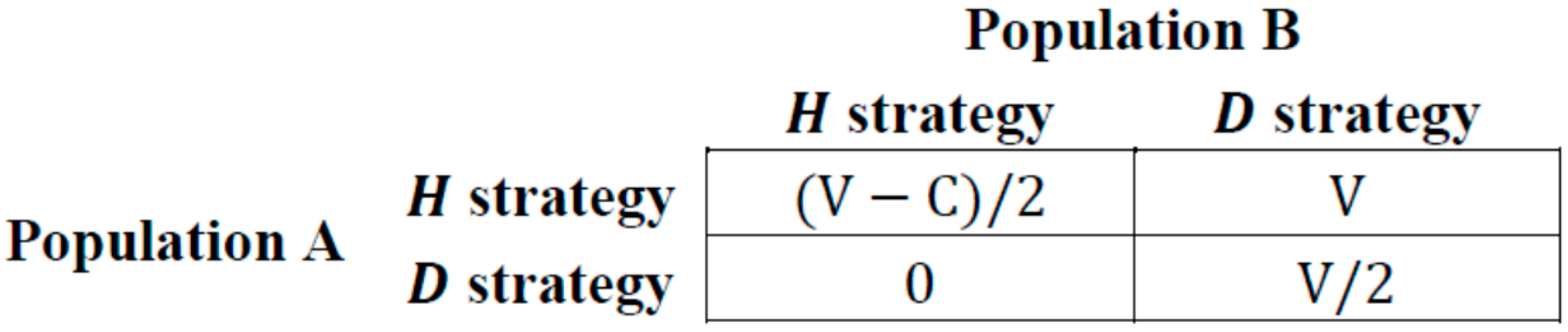
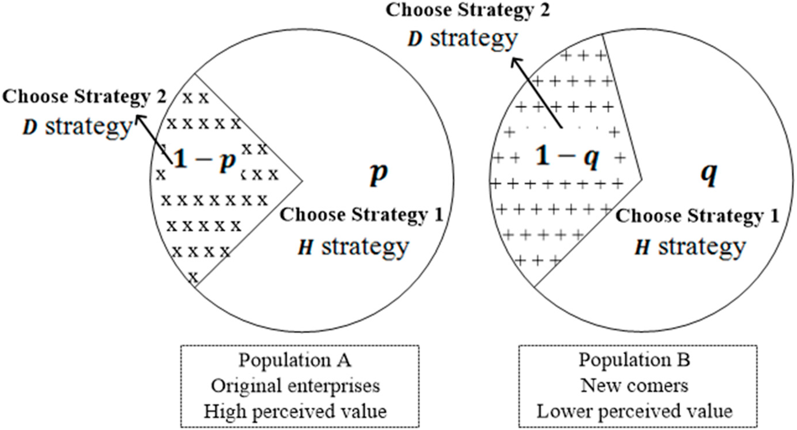
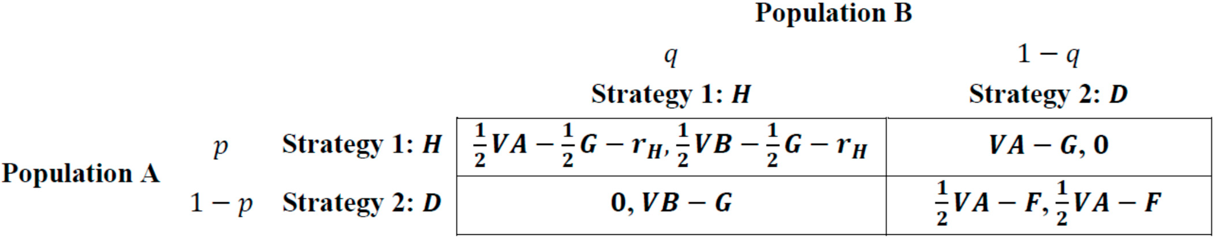
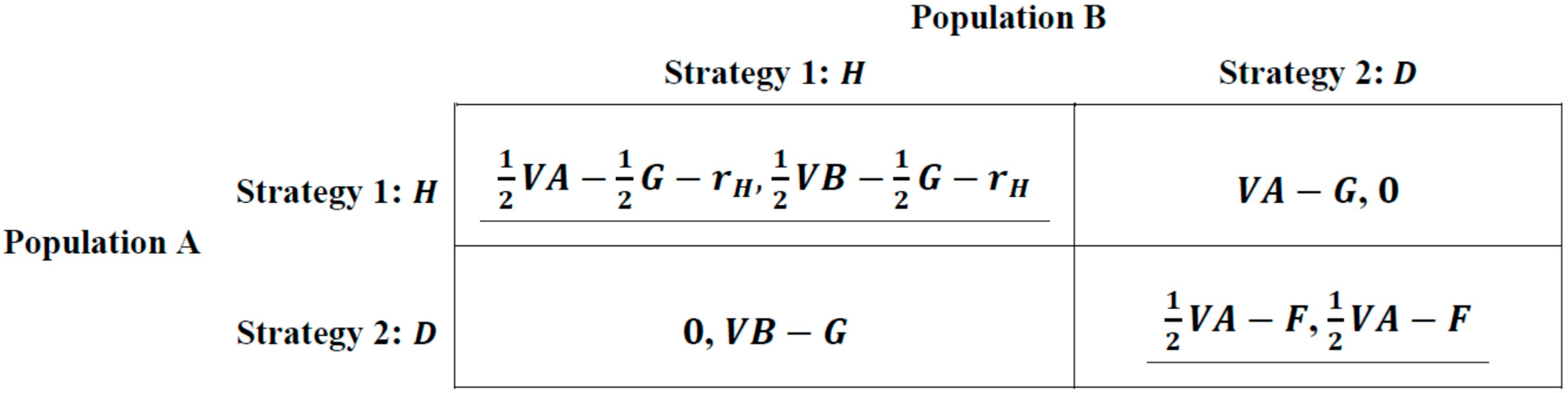
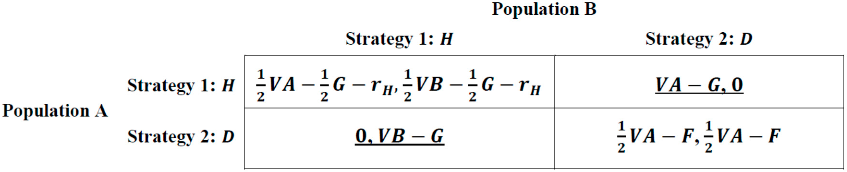
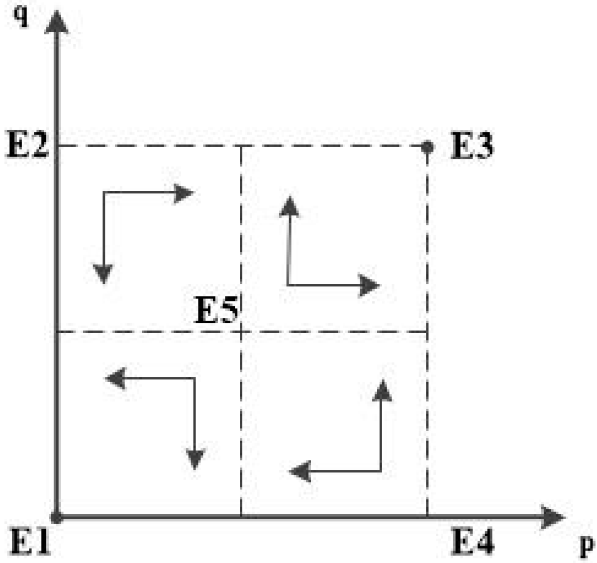
3. Evolutionary Game Analysis
3.1. Modeling


3.2. Results and Discussion


| Equilibrium Points | Det J and Tr J | PM | Results |
|---|---|---|---|
| E1(0,0) | + | ESS | |
| − | |||
| E2(0,1) | + | instable | |
| + | |||
| E3(1,1) | + | ESS | |
| − | |||
| E4(1,0) | + | instable | |
| + | |||
| − | Saddle Point | ||
| TrJ = 0 | 0 |

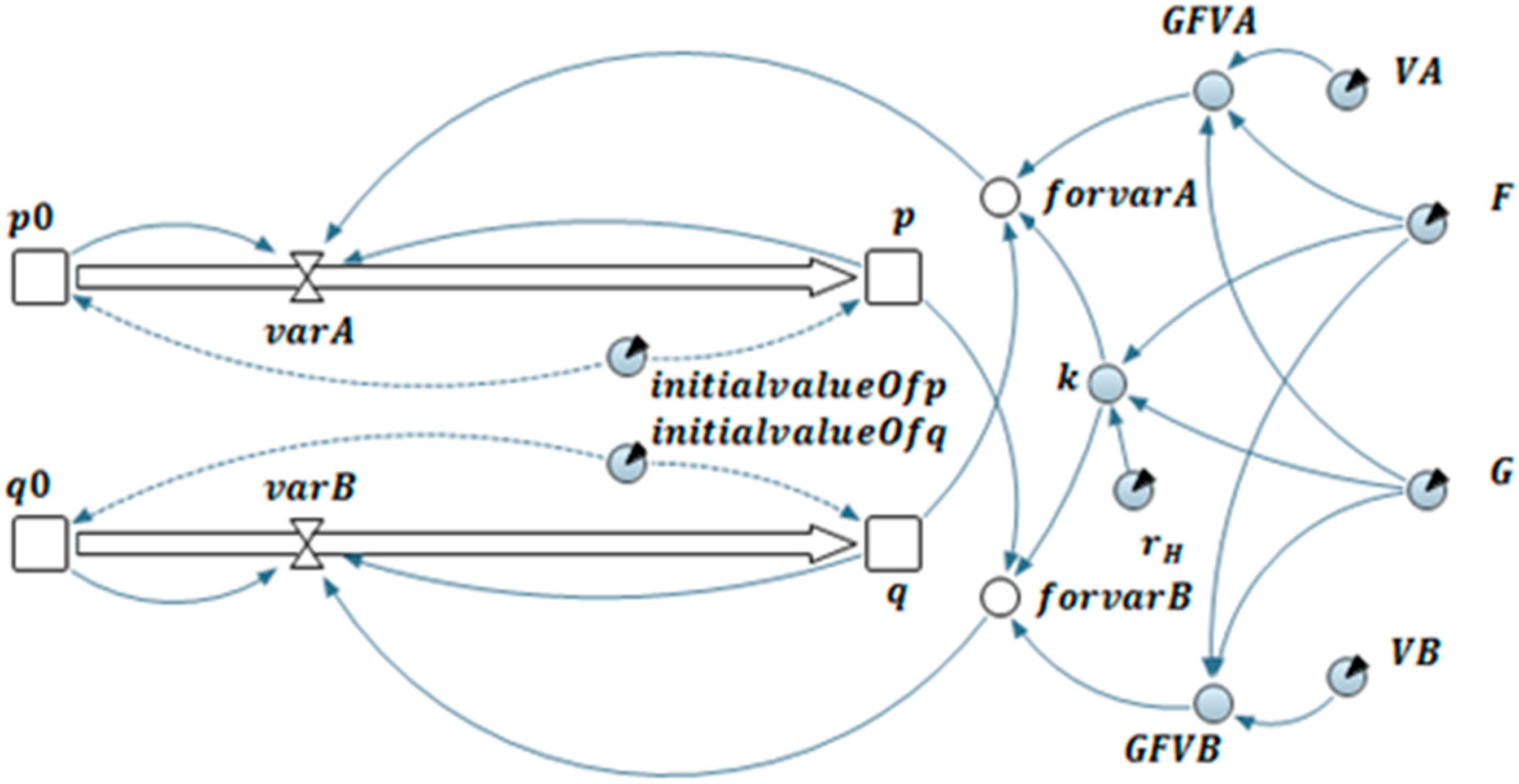
4. System Dynamics Simulation
4.1. Modeling and Parameter Design
- - Proportion of Population A choosing strategy
- - Proportion of Population B choosing strategy
- - Proportion of Population A choosing strategy, i.e.,
- - Proportion of Population B choosing strategy, i.e.,
- - The rate of changing with time
- - The rate of changing with time
- - Bidding related cost (unit: SC, “simulation currency”, without real meaning)
- - Price (unit: SC, “simulation currency”, without real meaning)
- - Penalty (unit: SC, “simulation currency”, without real meaning)
- - Perceived value of Population A (unit: SC, “simulation currency”, without real meaning)
- - Perceived value of Population B (unit: SC, “simulation currency”, without real meaning)
- - Initial value of
- - Initial value of

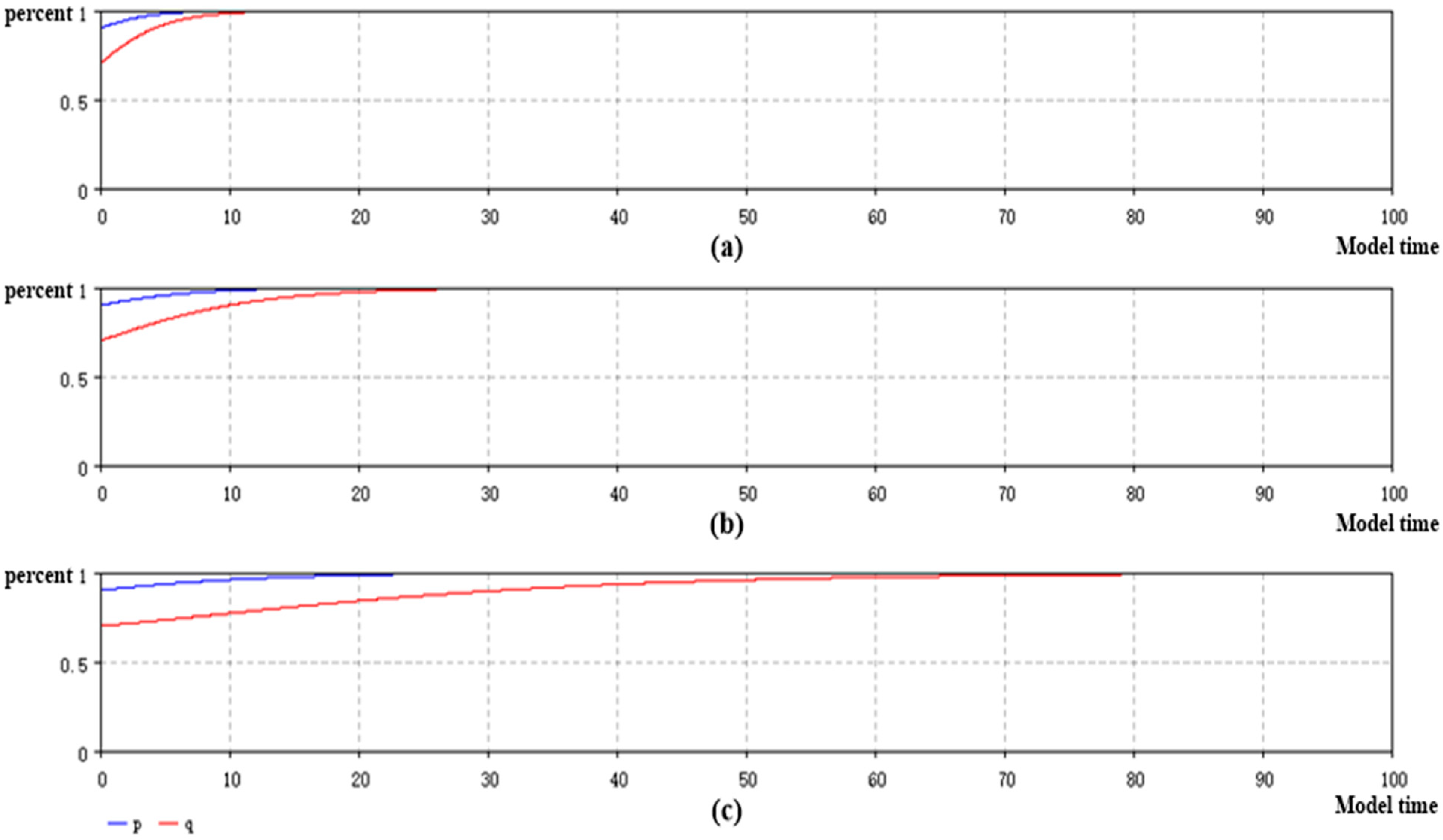
4.2. Preliminary Simulation Analysis
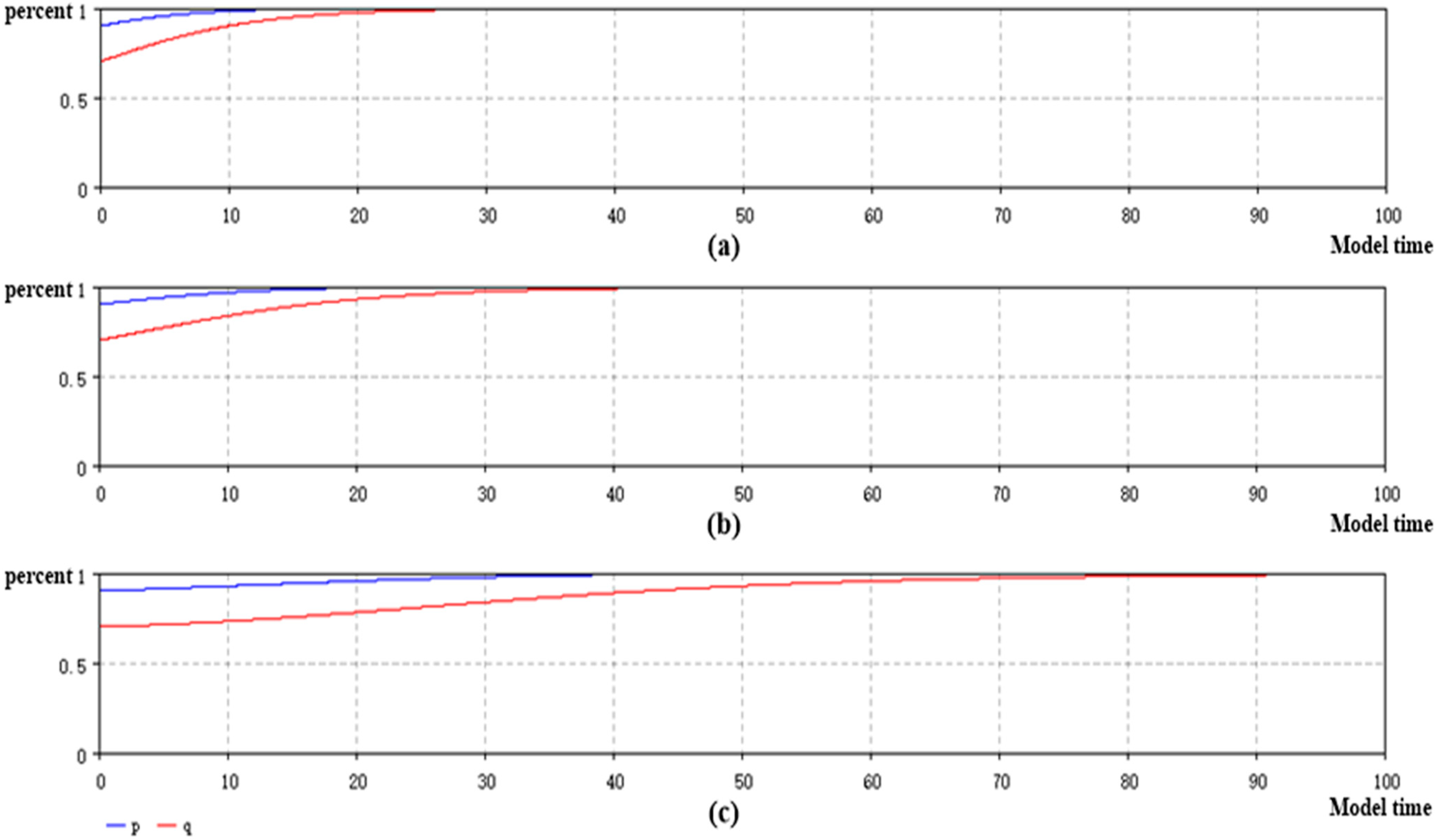
4.2.1. The Effect of on Rate of Convergence
| Number | p | q | VA | VB | G | F | rH |
|---|---|---|---|---|---|---|---|
| 4.2.1-1 | 0.9 | 0.7 | 2.1 | 1.9 | 1.2 | 0.1 | 0 |
| 4.2.1-2 | 0.9 | 0.7 | 2.1 | 1.9 | 1.2 | 0.1 | 0.2 |
| 4.2.1-3 | 0.9 | 0.7 | 2.1 | 1.9 | 1.2 | 0.1 | 0.3 |

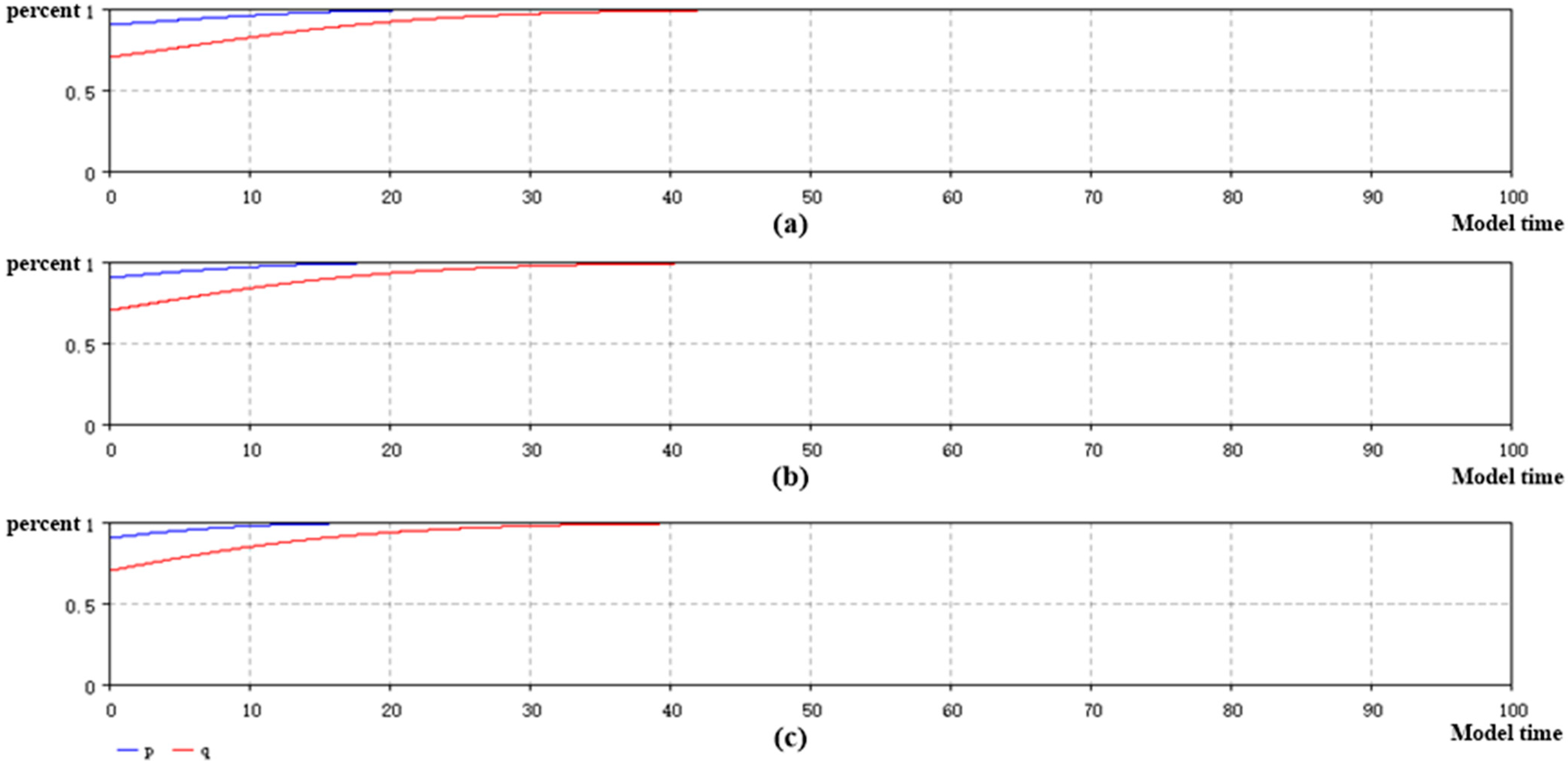
4.2.2. The Effect of on Rate of Convergence
| Number | p | q | VA | VB | G | F | rH |
|---|---|---|---|---|---|---|---|
| 4.2.2-1 | 0.9 | 0.7 | 2.1 | 1.9 | 1.2 | 0.1 | 0.2 |
| 4.2.2-2 | 0.9 | 0.7 | 2.1 | 1.9 | 1.3 | 0.1 | 0.2 |
| 4.2.2-3 | 0.9 | 0.7 | 2.1 | 1.9 | 1.4 | 0.1 | 0.2 |

4.2.3. The Effect of on Rate of Convergence

| Number | p | q | VA | VB | G | F | rH |
|---|---|---|---|---|---|---|---|
| 4.2.3-1 | 0.9 | 0.7 | 2.1 | 1.9 | 1.3 | 0 | 0.2 |
| 4.2.3-2 | 0.9 | 0.7 | 2.1 | 1.9 | 1.3 | 0.1 | 0.2 |
| 4.2.3-3 | 0.9 | 0.7 | 2.1 | 1.9 | 1.3 | 0.2 | 0.2 |
4.3. Advanced Simulation Analysis
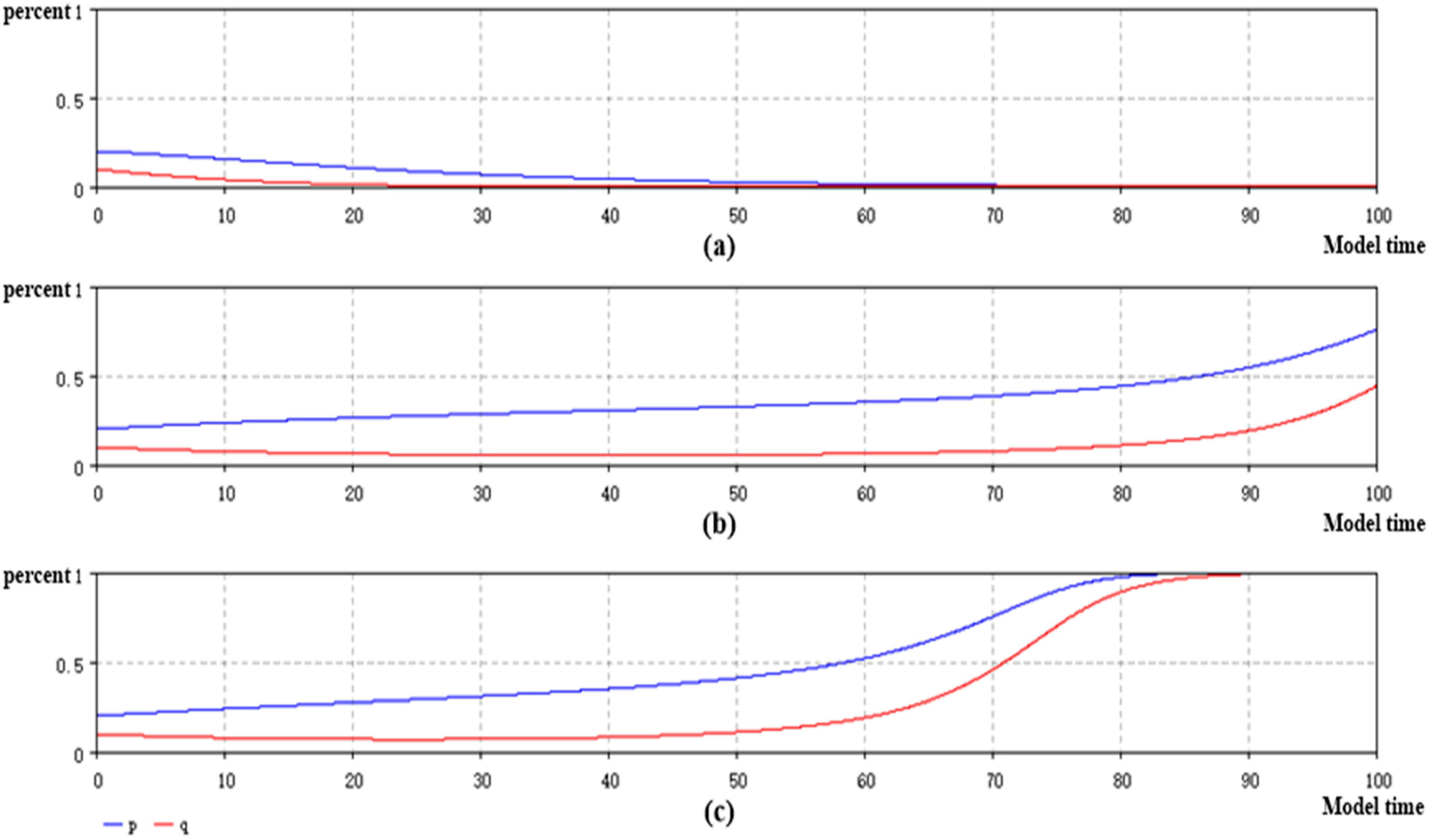
4.3.1. Test of Combined Effect of , and

| Number | p | q | VA | VB | G | F | rH |
|---|---|---|---|---|---|---|---|
| 4.3.1-1 | 0.2 | 0.1 | 2.1 | 1.9 | 1.2 | 0.1 | 0.2 |
| 4.3.1-2 | 0.2 | 0.1 | 2.1 | 1.9 | 1.2 | 0.14 | 0.1 |
| 4.3.1-3 | 0.2 | 0.1 | 2.1 | 1.9 | 1.16 | 0.1 | 0.1 |
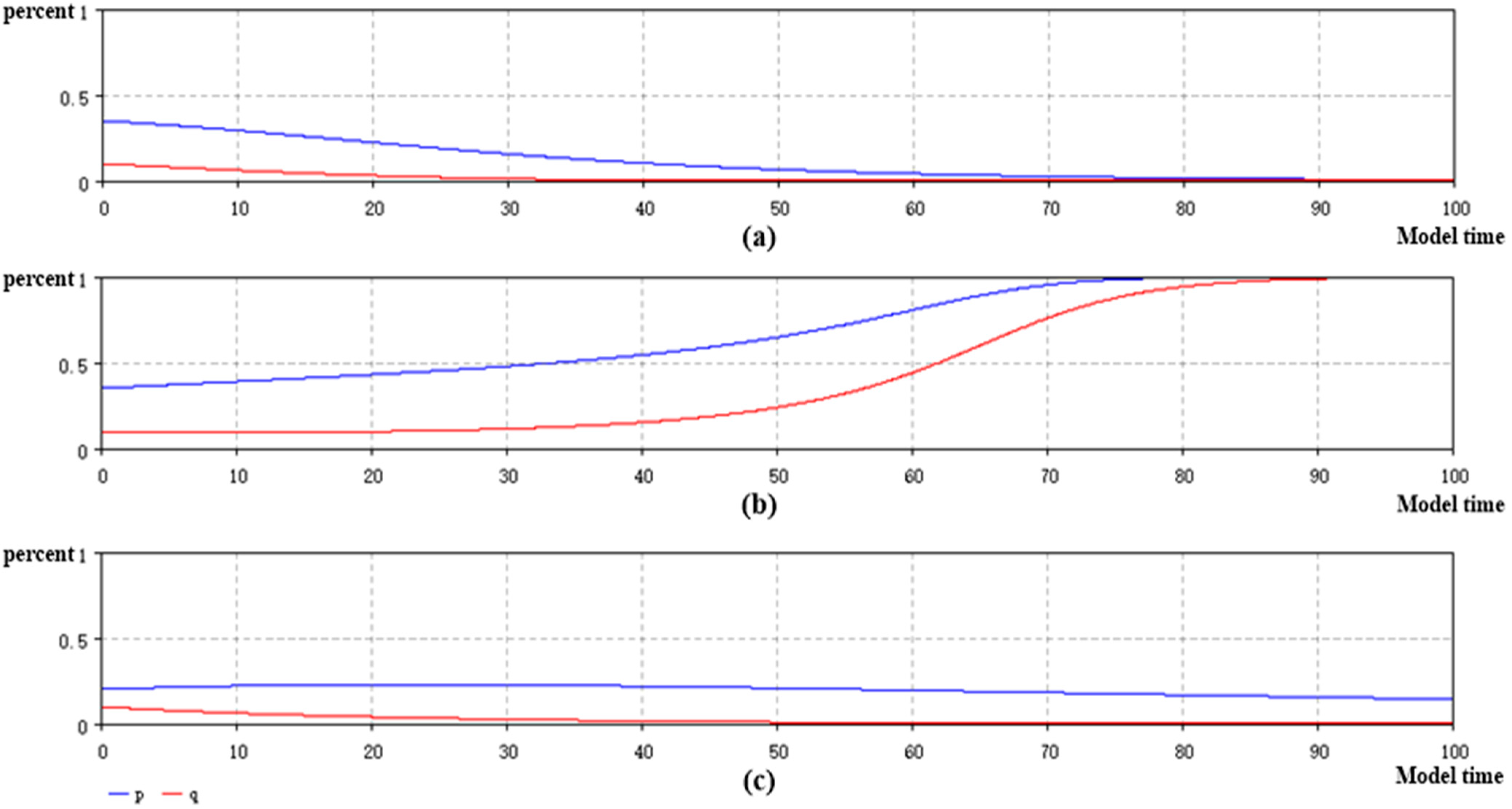
4.3.2. Discussion of

| Number | p | q | VA | VB | G | F | rH |
|---|---|---|---|---|---|---|---|
| 4.3.2-1 | 0.35 | 0.1 | 2.1 | 1.9 | 1.2 | 0.1 | 0.2 |
| 4.3.2-2 | 0.35 | 0.1 | 2.1 | 1.9 | 1.16 | 0.1 | 0.2 |
| 4.3.2-3 | 0.2 | 0.1 | 2.1 | 1.9 | 1.16 | 0.1 | 0.2 |
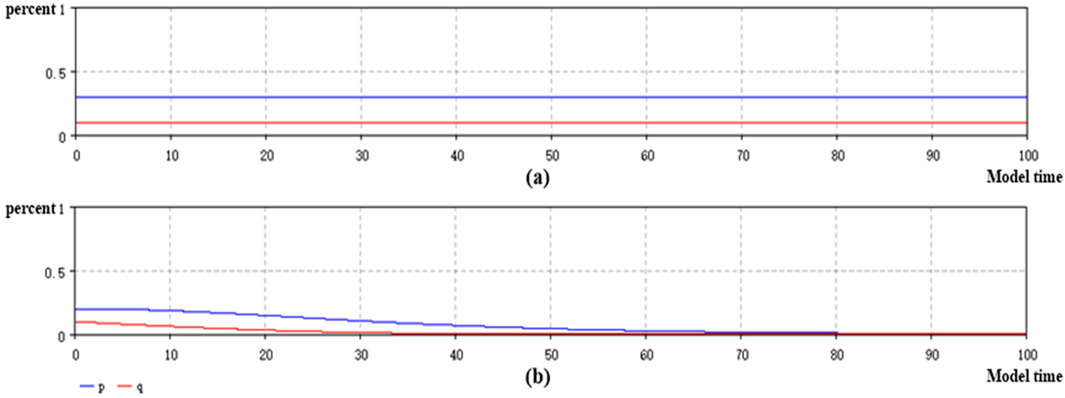
4.3.3 Discussion on Saddle Point

| Number | p | q | VA | VB | G | F | rH |
|---|---|---|---|---|---|---|---|
| 4.2.1-1 | 0.9 | 0.7 | 2.1 | 1.9 | 1.2 | 0.1 | 0 |
| 4.3.3-1 | 0.3 | 0.1 | 2.1 | 1.9 | 1.2 | 0.1 | 0 |
| 4.3.3-2 | 0.2 | 0.1 | 2.1 | 1.9 | 1.2 | 0.1 | 0 |
5. Conclusions
Acknowledgments
Author Contributions
Conflicts of Interest
References
- Wolf, C. China: Pitfalls on Path of Continued Growth. In China’s Continued Economic Progress: Possible Adversities and Obstacles, Proceedings of the 5th Annual CRF-RAND Conference, Beijing, China, 31 October–1 November 2002.
- Youth. Available online: http://js.youth.cn/20141110/611846.shtml (accessed on 10 November 2014).
- H2O-China. Available online: http://www.h2o-china.com/news/216428.html (accessed on 10 November 2014). (In Chinese)
- Cason, T.N.; Gangadharan, L. Transactions Costs in Tradable Permit Markets: An Experimental Study of Pollution Market Designs. J. Regul. Econ. 2003, 2, 145–165. [Google Scholar]
- Chartres, C.; Varma, S. Out of Water From Abundance to Scarcity and How to Solve the World’s Water Problem, 1st ed.; China Machine Press: Beijing, China, 2012; pp. 43–45. [Google Scholar]
- Finance Eastday. Available online: http://finance.eastday.com/c9/2014/1209/3026807517.html (accessed on 9 December 2014).
- News Sina. Available online: http://news.sina.com.cn/o/2014–12–23/210731319191.shtml (accessed on 23 December 2014).
- Zhang, C.; Diaz, A.L.; Mo, H.; Zhao, Z.; Liu, Z. Water-Carbon Trade-off in China’s Coal Power Industry. Environ. Sci. Technol. 2014, 19, 11082–11089. [Google Scholar] [CrossRef]
- Wang, Q.; Yuan, X.; Zuo, J.; Mu, R.; Zhou, L.; Sun, M. Dynamics of Sewage Charge Policies, Environmental Protection Industry and Polluting Enterprises–A Case Study in China. Sustainability 2014, 6, 4858–4876. [Google Scholar] [CrossRef]
- Tao, W.; Zhou, B.; Barron, W.F.; Yang, W. Tradable Discharge Permit System for Water Pollution: Case of the Upper Nanpan River of China. Environ. Resour. Econ. 2000, 15, 27–38. [Google Scholar] [CrossRef]
- Yuhuan-China-Government. Available online: http://sjj.yuhuan.gov.cn/sjwh/yswh/201306/t20130627_62268.htm (accessed on 23 December 2014).
- Hu, A.; Wang, Y. China’s Public Policy of Water Resources Allocation in Transition: Quasi-market, Political and Democratic Consultation. China Soft Sci. 2000, 5, 5–11. [Google Scholar]
- Beall, A.; Fiedler, F.; Boll, J.; Cosens, B. Sustainable Water Resource Management and Participatory System Dynamics. Case Study: Developing the Palouse Basin Participatory Model. Sustainability 2011, 3, 720–742. [Google Scholar]
- Rabotyagov, S.S.; Valcu, A.M.; Kling, C.L. Reversing Property Rights: Practice-Based Approaches for Controlling Agricultural Nonpoint-source Water Pollution When Emissions Aggregate Nonlinearly. Am. J. Agric. Econ. 2014, 2, 397–419. [Google Scholar] [CrossRef]
- Yin, M.; YuB, H.; Chen, Y. Key Technology and Allocation Pilot on Initial Water Right Distribution in River Basin, 1st ed.; China Water & Power Press: Beijing, China, 2012; pp. 154–196. [Google Scholar]
- Liu, J. Annual Report on Environment Development of China (2014), 1st ed.; Social Sciences Academic Press: Beijing, China, 2014; p. 132. [Google Scholar]
- Chen, L.; Zhang, S. Gaming Analysis for Behaviors of the Enterprises Involving Emission Trading. Acta Sci. Nat. Univ. Pekinensis 2005, 6, 926–934. [Google Scholar]
- Coase, R.H. The Problem of Social Cost. J. Law Econ. 1960, 10, 1–23. [Google Scholar] [CrossRef]
- Croker, T.D. The structuring of atmospheric pollution control system. Emiss. Trad. Progr. 2001, 5, 11–20. [Google Scholar]
- Dales, J.H. Pollution, Property and Prices: An Essay in Policy-Making and Economics, 3rd ed.; Edward Elgar Publishing Ltd: Cheltenham, UK, 2002; pp. 12–15. [Google Scholar]
- Douglas, C.M.; Klatt, P.J. Economic Design of T2 Control Charts to Maintain Current Control of a Process. Manag. Sci. 1972, 9, 76–89. [Google Scholar]
- Mesbah, S.M.; Kerachian, R.; Nikoo, M.R. Developing real time operating rules for trading discharge permits in rivers: Application of Bayesian Networks. Environ. Model. Softw. 2009, 24, 238–246. [Google Scholar] [CrossRef]
- Hahn, R.W.; Hester, G.L. Where did all the markets go? An analysis of EPA’s emission trading program. Yale J. Regul. 1989, 6, 109–153. [Google Scholar]
- Tietenberg, T.H. Economic instruments for environmental regulation. Oxf. Rev. Econ. Policy 1991, 6, 125–178. [Google Scholar]
- Zhang, J.L.; Li, Y.P.; Huang, G.H. A robust simulation-optimization modeling system for effluent trading-a case study of nonpoint source pollution control. Environ. Sci. Poll. Res. 2013, 7, 5036–5053. [Google Scholar]
- Andrew, J.Y.; Doyle, M.W.; Rigby, J.R.; Schnier, K.E. Market power, private information, and the optimal scale of pollution permit markets with application to North Carolina’s Neuse River. Resour. Energy Econ. 2013, 35, 256–276. [Google Scholar] [CrossRef]
- Atkinson, S.E.; Tietenberg, T.H. Market failure in incentive based regulation: The case of emission trading. J. Environ. Econ. Manag. 1991, 21, 17–31. [Google Scholar] [CrossRef]
- Milliman, S.; Prince, R. Firm incentives to promote technological change in pollution control. J. Environ. Econ. Manag. 1989, 16, 156–166. [Google Scholar] [CrossRef]
- Jung, C.; Krutilla, K.; Boyd, R. Incentives for advanced pollution abatement technology at the industry level: An evaluation of policy alternatives. J. Environ. Econ. Manag. 1996, 30, 95–111. [Google Scholar] [CrossRef]
- Ai, J. Equilibrium Analysis of Emission Trading Market Based on Evolutionary Game. Stat. Decis. 2011, 11, 67–69. [Google Scholar]
- Ning, S.-K.; Chang, N.-B. River Basin-Based Point Sources Permitting Strategy and Dynamic Permit-Trading Analysis. J. Environ. Manag. 2007, 84, 427–446. [Google Scholar] [CrossRef]
- Chen, J.; Xu, C.; Tian, G. Analysis the Efficiency of Water Rights Distribution in China. China Popul. Resour. Environ. 2006, 16, 49–53. [Google Scholar]
- Videira, N.; Antunes, P.; Santos, R. Scoping river basin management issues with participatory modelling: the Baixo Guadiana experience. Ecol. Econ. 2009, 68, 965–978. [Google Scholar] [CrossRef]
- Fernald, A.; Tidwell, V.; Rivera, J.; Rodríguez, S.; Guldan, S.; Steele, C.; Ochoa, C.; Hurd, B.; Ortiz, M.; Boykin, K.; et al. Modeling Sustainability of Water, Environment, Livelihood, and Culture in Traditional Irrigation Communities and Their Linked Watersheds. Sustainability 2012, 4, 2998–3022. [Google Scholar] [CrossRef]
- Sun, T.; Zhang, H.; Wang, Y.; Meng, X.; Wang, C. The application of environmental Gini coefficient (EGC) in allocating wastewater discharge permit: The case study of river basin total mass control in Tianjin. China Resour. Conserv. Recycl. 2010, 54, 601–608. [Google Scholar] [CrossRef]
- Skardi, M.J.E.; Afshar, A.; Solis, S.S. Simulation-Optimization Model for Non-point Source Pollution Management in River basins: Application of Cooperative Game Theory. J. Civil Eng. 2013, 17, 1232–1240. [Google Scholar]
- Teasley, R.L.; McKinney, D.C. Calculating the Benefits of Transboundary River Basin Cooperation: Syr Darya Basin. J. Water Resour. Plan. Manag. 2011, 137, 481–490. [Google Scholar] [CrossRef]
- Lee, C.-S. Multi-objective game-theory models for conflict analysis in reservoir river basin management. Chemosphere 2012, 87, 608–613. [Google Scholar] [CrossRef] [PubMed]
- Nguyen, N.P.; Shortle, J.S.; Reed, P.M.; Nguyen, T.T. Water quality trading with asymmetric information, uncertainty and transaction costs: A stochastic agent-based simulation. Resour. Energy Econ. 2013, 35, 60–90. [Google Scholar] [CrossRef]
- López-Villarreal, F.; Lira-Barragán, L.F.; Rico-Ramirez, V.; Ponce-Ortega, J.M.; El-Halwagi, M.M. An MFA optimization approach for pollution trading considering the sustainability of the surrounded river basins. Comput. Chem. Eng. 2014, 63, 140–151. [Google Scholar] [CrossRef]
- Gani, A.; Scrimgeour, F. Modeling governance and water pollution using the institutional ecological economic framework. Econ. Model. 2014, 42, 363–372. [Google Scholar] [CrossRef]
- Madani, K. Game theory and water resources. J. Hydrol. 2010, 381, 225–238. [Google Scholar] [CrossRef]
- Piscopo, K.; Varga, S. Dynamic Stackelberg game model for water rationalization in drought emergency. J. Hydrol. 2014, 517, 557–565. [Google Scholar] [CrossRef]
- Li, S.; Xue, Y. Analyzing the Non-cooperation Game between the Enterprise and Environmental Regulator under Emission Trading Institution. J. Taiyuan Univ. Sci. Technol. 2005, 26, 233–236. [Google Scholar] [CrossRef]
- Weibull, J.W. Evolutionary Game Theory, 1st ed.; Chen, X., Ed.; Shanghai People’s Publishing House: Shanghai, China, 2006; Volume 1, p. 3. [Google Scholar]
- Wang, X.; Quan, J.; Liu, W. Study on Evolutionary Games and Cooperation Mechanism within the Framework of Bounded Rationality. Syst. Eng.-Theory Pract. 2011, 31, 82–93. [Google Scholar]
- Weibull, J.W. Evolutionary Game Theory, 1st ed.; Chen, X., Ed.; Shanghai People’s Publishing House: Shanghai, China, 2006; Volume 1, p. 5. [Google Scholar]
- Chen, Z.; Wang, H.; Qiu, L.; Chen, J. Evolutionary Game Analysis of Water Resources Allocation in River Basin. Chin. J. Manag. Sci. 2008, 16, 176–183. [Google Scholar]
- Yu, R.; Wang, H.; Niu, W. Evolutionary Game Analysis of Price Competition Strategy for Water Market. In Advanced Materials Research, Proceedings of the International Conference on Civil Engineering and Building Materials (CEBM), Kunming, China, 29–31 July 2011; Zhao, J.Y., Ed.; Trans Tech Publications Ltd.: Zurich, Switzerland, 2011. [Google Scholar]
- Li, C.; Zhang, L.; Zhao, G.; Mo, L. Research on Basin Ecological Compensation Based on Evolutionary Game Theory-Taking Taihu Basin as a Case. China Popul. Res. Environ. 2014, 24, 171–176. [Google Scholar]
- Smith, J.M. Basic Model. In Evolution and the Theory of Games, 1st ed.; Pan, C., Wang, X., Eds.; Fudan University Press: Shanghai, China, 2008; Volume 1, p. 13. [Google Scholar]
- Friedman, D. On Economic Applications of Evolutionary Game Theory. J. Evol. Econ. 1998, 8, 15–43. [Google Scholar] [CrossRef]
- Sun, Q.; Lu, L.; Yan, G.; Che, H. Asymptotic Stability of Evolutionary Equilibrium under Imperfect Knowledge. Syst. Eng. Theory Pract. 2003, 7, 11–16. [Google Scholar]
- Sterman, J.D. Business Dynamics, Systems Thinking and Modeling for a Complex World; McGraw-Hill: Boston, MA, USA, 2000. [Google Scholar]
- Vennix, J.A.M. Group Model Building. Facilitating Team Learning Using System Dynamics; John Wiley and Sons: New York, NY, USA, 1996. [Google Scholar]
- Saysel, A.K.; Barlas, Y.; Yenigün, O. Environmental sustainability in an agricultural development project: A system dynamics approach. J. Environ. Manag. 2002, 64, 247–260. [Google Scholar] [CrossRef]
- Roach, J.; Tidwell, V. A compartmental-spatial system dynamics approach to ground water modeling. Ground Water 2009, 47, 686–698. [Google Scholar]
- Stave, K.A. System dynamics model to facilitate public understanding of water management options in Las Vegas, Nevada. J. Environ. Manag. 2003, 67, 303–331. [Google Scholar] [CrossRef]
- Stave, K. 2010 Participatory System Dynamics Modeling for Sustainable Environmental Management: Observations from Four Cases. Sustainability 2010, 2, 2762–2784. [Google Scholar] [CrossRef]
- Winz, I.; Brierley, G.; Trowsdale, S. The use of system dynamics simulation in water resources management. Water Resour. Manag. 2009, 23, 1301–1323. [Google Scholar] [CrossRef]
- World Bank; Chinese Academy of Sciences; Ministry of Water Resources of the PRC. Exploration and Practice of Soil and Water Conservation in China. In Proceedings of the Seminar on Small Watershed Sustainable Development, Beijing, China, 20–21 November 2005; China Water & Power Press: Beijing, China, 2005. [Google Scholar]
© 2015 by the authors; licensee MDPI, Basel, Switzerland. This article is an open access article distributed under the terms and conditions of the Creative Commons Attribution license (http://creativecommons.org/licenses/by/4.0/).
Share and Cite
Liu, L.; Feng, C.; Zhang, H.; Zhang, X. Game Analysis and Simulation of the River Basin Sustainable Development Strategy Integrating Water Emission Trading. Sustainability 2015, 7, 4952-4972. https://doi.org/10.3390/su7054952
Liu L, Feng C, Zhang H, Zhang X. Game Analysis and Simulation of the River Basin Sustainable Development Strategy Integrating Water Emission Trading. Sustainability. 2015; 7(5):4952-4972. https://doi.org/10.3390/su7054952
Chicago/Turabian StyleLiu, Liang, Cong Feng, Hongwei Zhang, and Xuehua Zhang. 2015. "Game Analysis and Simulation of the River Basin Sustainable Development Strategy Integrating Water Emission Trading" Sustainability 7, no. 5: 4952-4972. https://doi.org/10.3390/su7054952