4.1. Model Calibration and Validation
A model provides reliable results, in accordance with any recorded data, identifying appropriate parameter values that ensure an overall good agreement between recorded and simulated data. This process in principle should include independent phases of “calibration” and “validation”, in order to provide a model able to predict the quality-quantity response of basin for any flowed rainfall.
Nevertheless, the comparison between the flow rates simulated by the SWMM model and flow rates measured at the drainage system’s outlet for the three monitored events provided unexpected results after the calibration/validation procedure.
The parameters of the hydraulic model are: depth of depression storage on the impervious (Dstore-Imperv) and pervious (Dstore-Perv) portion of the subcatchment, Manning’s coefficient for overland flow over the impervious portion of the subcatchment (N-Imperv), Manning’s coefficient for overland flow over the pervious portion of the subcatchment (N-Perv), Percent of the impervious area with no depression storage (%Zero Imperv) and the characteristic width of the overland flow path for sheet flow runoff (Width) [
27]. Their range of variation (e.g., [
28,
29]) and the values chosen for these parameters in this paper are shown in
Table 4.
In particular:
- -
the values of Dstore-Imperv and Dstore-Perv, were fixed near the lower bound of the respective intervals, because in a urban basin we expect that the runoff value is quite high; for the same reason we chose a mean-low value of the %Zero Imperv.
- -
the value of N-Imperv was fixed equal to 0.012 s/m1/3, being the impervious surface characterized by smooth concrete material; moreover, the value of N-Perv was fixed equal to 0.15 s/m1/3 being the pervious area characterized by grass short and prairie;
- -
the value of the Width of the overland flow path for sheet flow runoff, was evaluated taking into account the following [
30] formula valid for irregular shape basins:
where
W is the Width of the overland flow path [m],
Sk is the skew factor,
l [m] is the overland flow path.
To evaluate the
Sk value (0 <
Sk < 1), we used the following equation:
Where
A1 is the portion of area on one side of the overland flow path;
A2 is the portion of area on the other side;
Atot is the total area.
Table 4.
Parameters of the hydraulic-hydrological model.
Table 4.
Parameters of the hydraulic-hydrological model.
| Parameters | Description | Range | Value |
|---|
| Dstore-Imperv | Depth of depression storage on the impervious portion of the subcatchment [mm] | 1.27–2.54 * | 1.30 |
| Dstore-Perv | Depth of depression storage on the pervious portion of the subcatchment [mm] | 2.54–5.08 * | 2.60 |
| N-Imperv | Manning’s coefficient for overland flow over the impervious portion of the subcatchment [s/m1/3] | 0.011–0.024 ** | 0.012 |
| N-Perv | Manning’s coefficient for overland flow over the pervious portion of the subcatchment [s/m1/3] | 0.15–0.41 ** | 0.15 |
| % Zero Imperv | Percent of the impervious area with no depression storage [%] | | 45 |
| Width | Characteristic width of the overland flow path for sheet flow runoff [m] | | Subcatchment 1 | 335 |
| Subcatchment 2 | 717 |
| Subcatchment 3 | 527 |
| Subcatchment 4 | 378 |
| Subcatchment 5 | 483 |
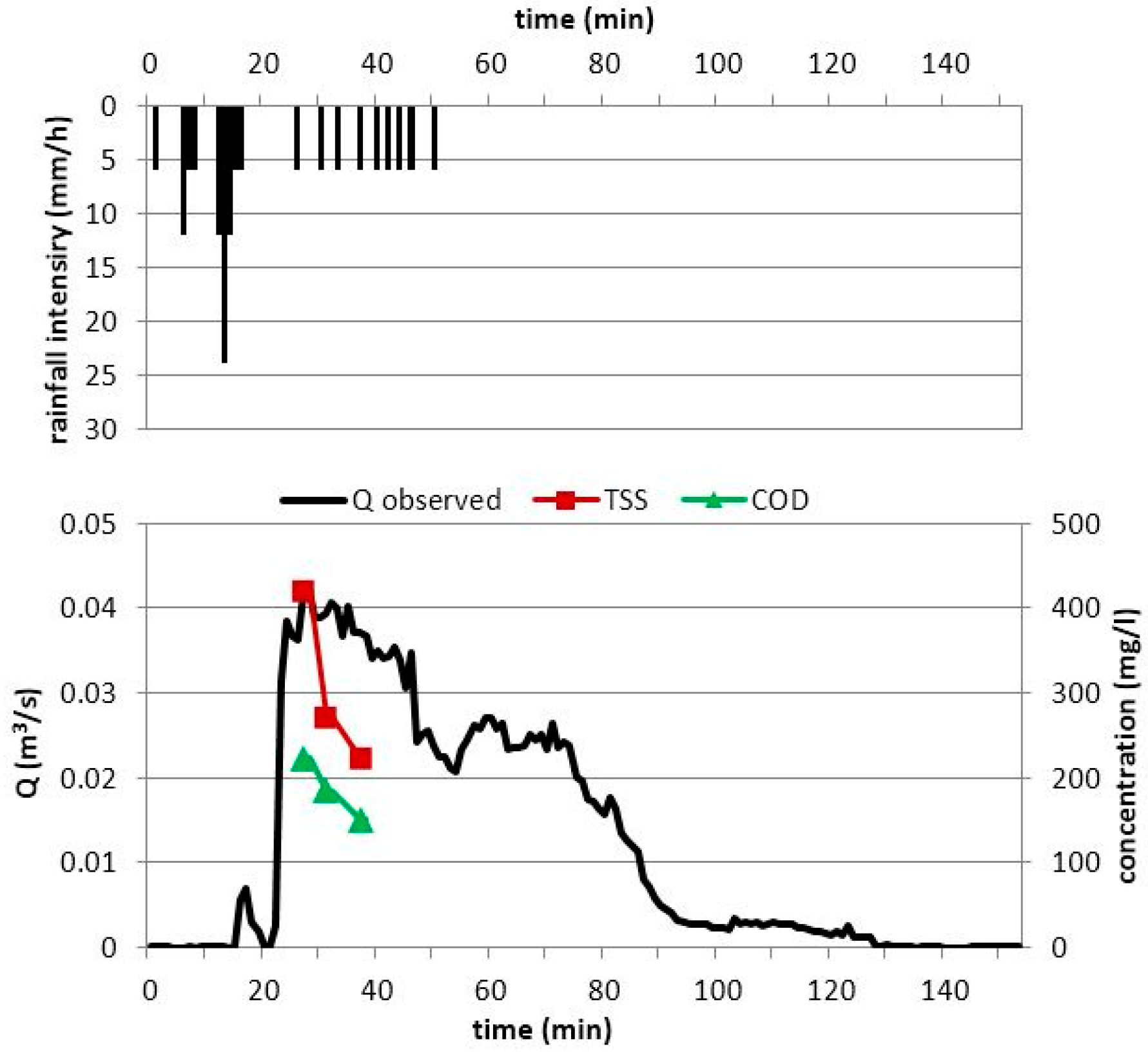
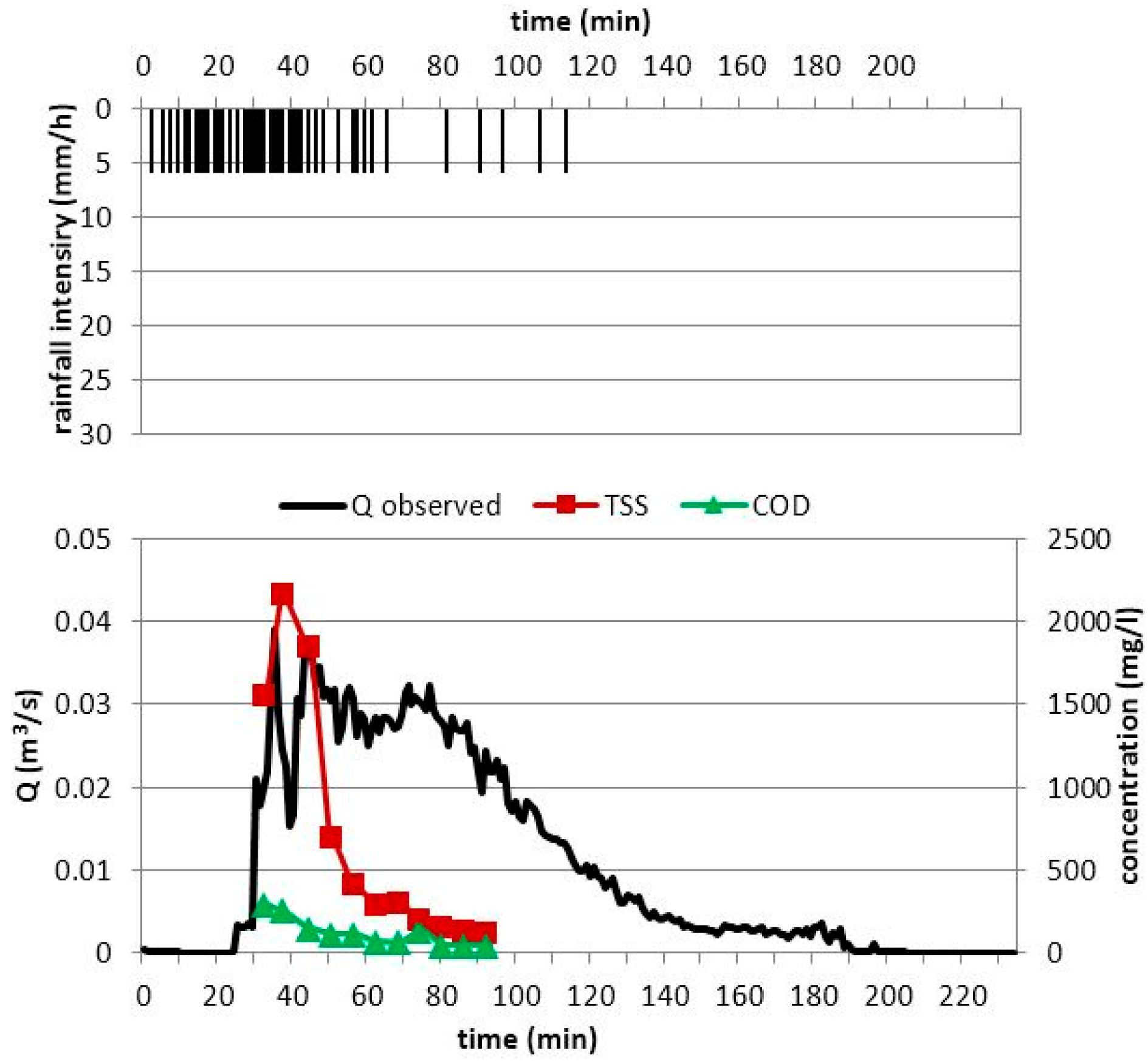
Initially, we tried to use the first of the three observed events for calibration and the others for validation. Nevertheless, based on the contemporary measures of rainfall and discharge, and even after different choices for the calibration event, we found a poor agreement as shown in
Figure 10. The simulated flow rates are always higher than the measured, unless we use some parameter values that are outside their suitable physical range. As shown in
Figure 10, the observed peak discharge assumes values close to 0.04 m
3/s (in the events of 10 November 2006 and 22 November 2006) and 0.05 m
3/s (event of 24 January 2007) which is totally uncorrelated with either rainfall depth or peak of rainfall intensity. These observations proves that the drainage system was unable to capture the entire generated runoff probably because of a shortage, wrong position, obstruction of inlet catch basins or due to losses in the network. As a matter of fact, the sewer system has been object of works to improve its drainage efficiency in 2008.
Figure 10.
Comparison between observed flow rates (blue line) and simulated ones (red line) for the event (a) 10 November, 2006; (b) 22 November, 2006; (c) 24 January, 2007.
Figure 10.
Comparison between observed flow rates (blue line) and simulated ones (red line) for the event (a) 10 November, 2006; (b) 22 November, 2006; (c) 24 January, 2007.
In order to preserve and exploit the scientific value of the pollutant sampling, we performed a sensitivity analysis of the parameter rc which settles the characteristics of the pollutant transport into the sewer system. Considering the rainfall input of the three observed events we found that for rc values within the typical range of literature for urban areas, the pollutant concentrations at the inlet of the drainage network remains practically unaffected by processes that develop within the drainage network. In other words, the transport process in this drainage system does not alter significantly the TSS concentration, which depends substantially on the washoff and build up phenomena, for rainfall events of characteristics (antecedent dry period, intensity, duration, etc.) similar to those observed.
Following these considerations and assuming that the flow conveyed in the drainage network, is a part of the hydrological flow, we performed the model calibration and validation with reference to the TSS concentration data measured at the drainage system’s outlet, during the three rainfall events monitored. As mentioned before, most of the surface is intended for residential use and is impervious, while only 3.8% of the basin is covered by urban-green. We observed that varying parameters of the buildup and wash-off model of the latter land use and TSS concentration measured at the drainage system’s outlet does not change; therefore, urban-green land use does not affect the model calibration process.
During the field campaign only three events were observed then, the first one (November 10
th, 2006) was used to calibrate model parameters while the other two events were used for model validation. Considering the very limited number of observed events assumed for most of the model parameters some reference literature values are detailed in
Section 2. Thus, we reduced as much as possible the number of calibration parameters. Quality-parameter values obtained in the calibration event are presented in
Table 5.
Table 5.
Parameter used for the quality calibration of the model.
Table 5.
Parameter used for the quality calibration of the model.
| Parameters | Range | Value |
|---|
| Buildup | Accu [kg/(ha·d)] | 10/25 * | 13.143 |
| Disp [1/d] | 0.08 ** | 0.08 |
| Wash off | Arra [1/mm] | 0.11/0.19 | 0.18 |
| Wash | 0/3 | 2.35 |
The calibration was made by means of an iterative process of trial and error, by adjusting the parameters in
Table 5. Working within the established range, and comparing (numerically and graphically) the simulation with the measured pollutograph, the calibration was worked on until a good fit was obtained. The numerical comparison was made by evaluating RMSE and
R2 per each rainfall event (
Table 6).
Table 6.
Numerical comparison between the simulated and measured pollutographs for each rainfall event.
Table 6.
Numerical comparison between the simulated and measured pollutographs for each rainfall event.
| Events | RMSE | R2 |
|---|
| Calibration: 11/10/2006 | 30.92 | 0.994 |
| Validation: 11/22/2006 | 663.30 | 0.670 |
| Validation: 01/24/2007 | 57.48 | 0.967 |
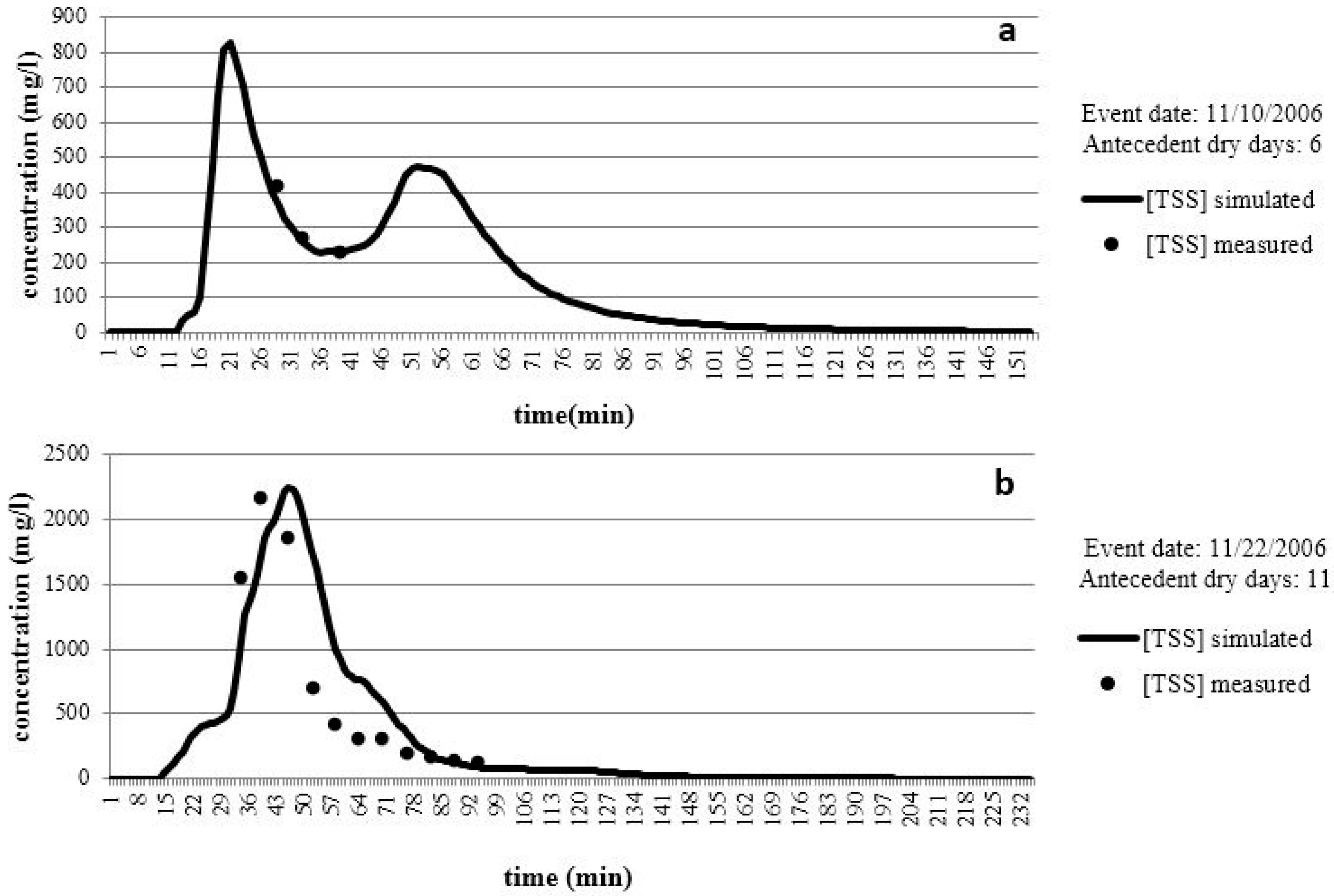
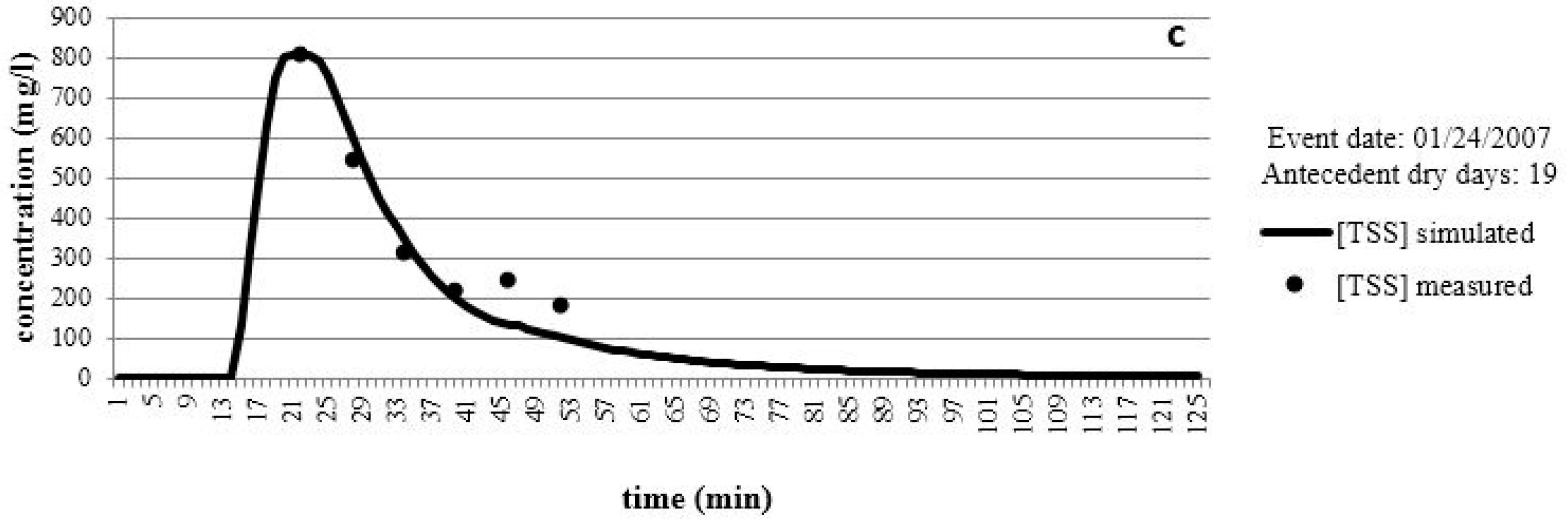
As we can see in
Figure 11, the simulated pollutographs very well interpolate the values of TSS concentration measured during the calibration event of 10 November 2006 and also during the validation event of 24 January 2007. A still fair comparison is obtained for the second validation event of 22 November 2006 which provides a high value of RMSE which seems mainly due to a shift in the peak time; in fact, the maximum observed value (2160 mg/L) is not far from the simulated peak value (2231 mg/L).
Figure 11.
Comparison between TSS concentrations of measured and simulated data of the calibration event: (a) 10 November 2006; and validation events: (b) 22 November 2006; (c) 24 January 2007.
Figure 11.
Comparison between TSS concentrations of measured and simulated data of the calibration event: (a) 10 November 2006; and validation events: (b) 22 November 2006; (c) 24 January 2007.
4.2. Analysis of the First Flush Occurrence
The monitoring process conducted in this study, allowed the analysis of the distribution of pollutant mass
vs. volume in stormwater discharges in dimensionless terms by using the so-called “M(V) curves” [
10]. This representation provides the variation of the cumulative pollutant mass divided by the total pollutant mass in relation to the cumulative volume divided by the total volume. If the concentration remains constant during the storm event, the pollutant mass is proportional to the volume and the M(V) curve is merged with the 1:1 line. When the M(V) curve is above the 1:1 line, the first-flush is noticed and the extent of the phenomenon increases with the slope of the curve for small values of volume.
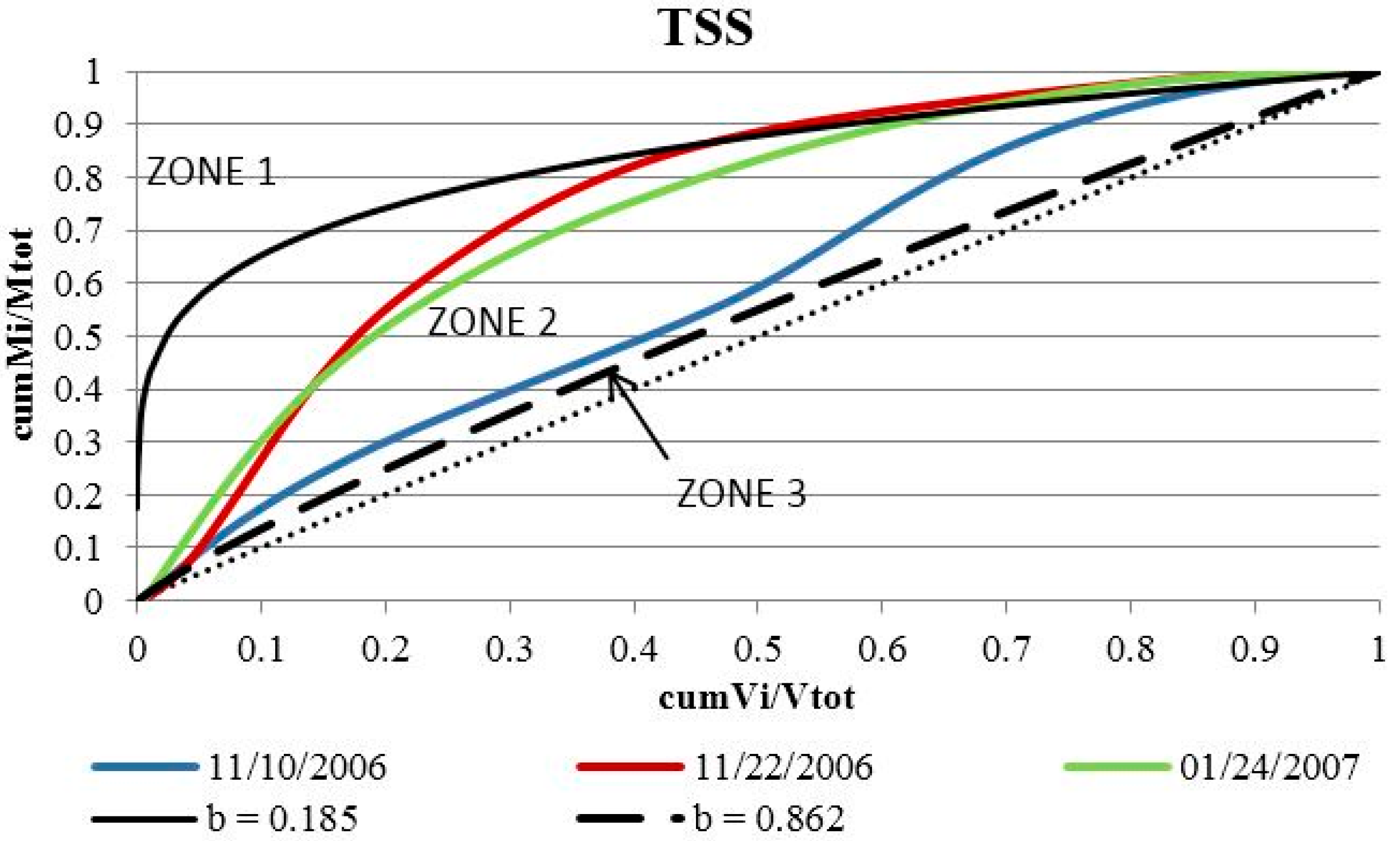
The M(V) curves obtained from TSS data processing of the three events recorded in Sannicandro di Bari are shown in
Figure 12.
Figure 12.
M(V) curves for TSS relating to the three events recorded in Sannicandro di Bari.
Figure 12.
M(V) curves for TSS relating to the three events recorded in Sannicandro di Bari.
Comparing the three events, which differ mainly in terms of antecedent dry period (
Table 7), we observe the expected dependence of the first flush phenomenon on this factor.
Every M(V) curve can be fitted approximately by a power function [
10]:
The value of the parameter b characterizes the gap between the M(V) curve and the 1:1 line. The numerical analysis conducted on the parameter b indicates that it varies significantly from one event to another. It should also be noted here that the lower the value of b, the more pronounced is the first flush, being a high fraction of the total pollutant load transported during an early stage of the rainfall event.
Table 7.
Characteristics of three events in Sannicandro di Bari.
Table 7.
Characteristics of three events in Sannicandro di Bari.
| Events | Antecedent Dry Period (d) | Qmax (m3/s) |
|---|
| 11/10/2006 | 6 | 0.04 |
| 11/22/2006 | 11 | 0.04 |
| 01/24/2007 | 19 | 0.05 |
The parameter b allows the upper part of M(V) graph to be divided into three zones, delimited in
Figure 12 by a black solid line with b = 0.185 and a dotted black line with b = 0.862.
Zone 1 represents a phenomenon of a very pronounced first flush, with about 75% of pollutant mass and about 20% of runoff volume. Zone 2 represents the situations in which during the rainfall event the discharged concentration decreases (first flush phenomenon). Zone 3 is close to the 1:1 line, representing the zone where the pollutant mass concentration is more or less constant during the event. The curves representing the three events are in zone 2.
Furthermore, we know that the first flush phenomenon implies that most of the pollutant mass is washed off by the first inputs of a rainfall event. In fact, analyzing the M(V) curves for the three events examined, we can see that the first 30% of the volume of washed off water carries a quantity of TSS respectively equal to:
40% for the 10 November 2006 event;
70% for the 22 November 2006 event;
65% for the 24 January 2007 event.
Such results are in accordance with Lee
et al. [
31] who stated that first flush occurs strongly when the proportion of impervious area increases, considering the high proportion of impervious area (70%) of the catchment.
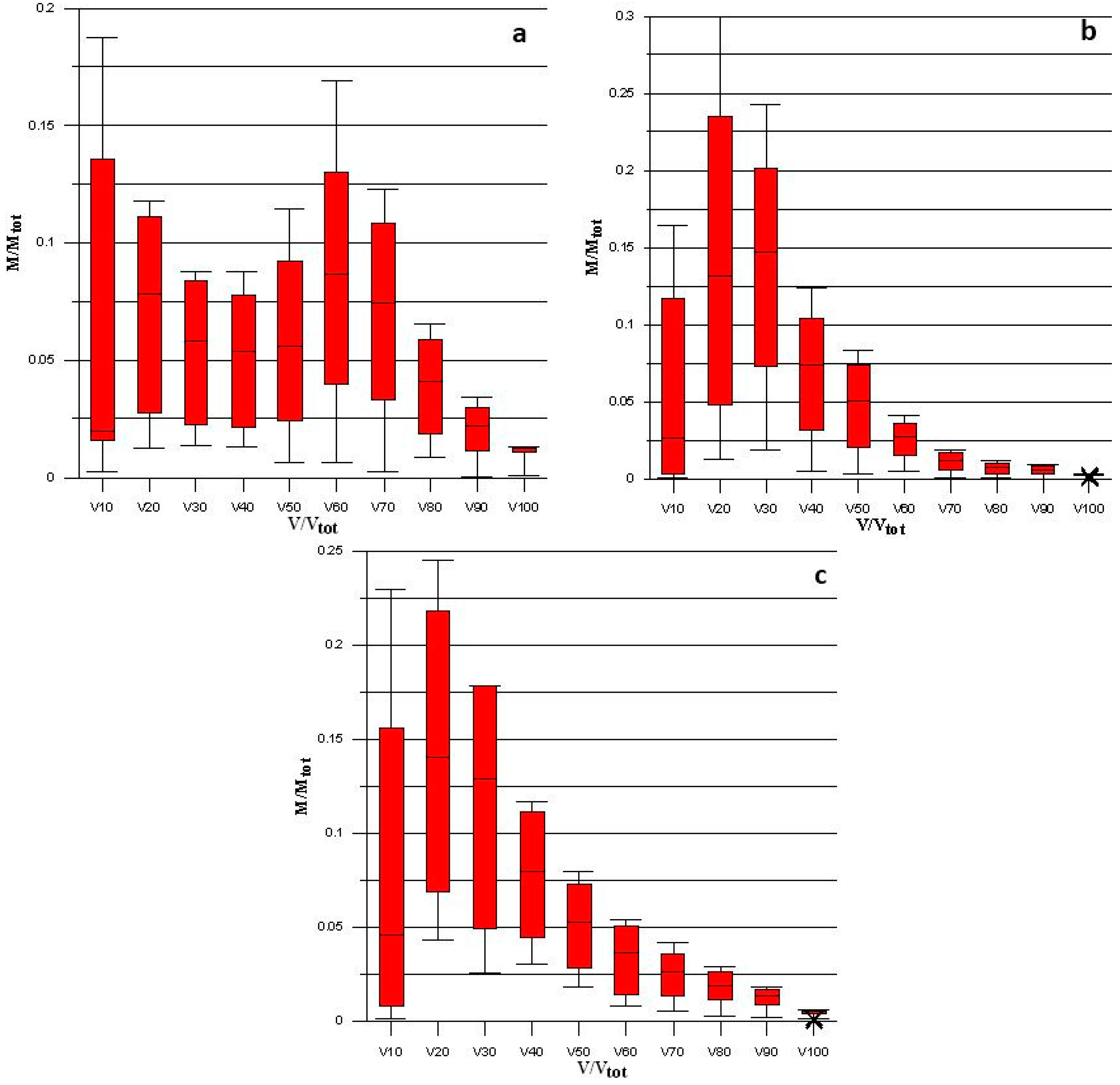
An alternative way to assess the occurrence of the first flush phenomenon is a comparison between the normalized pollutant mass emissions
vs. the normalized flow volume as shown in
Figure 13, where the normalized TSS mass emission rate is plotted for each normalized runoff volume ranging from 10%–100% with intervals of 10%.
From
Figure 13, we evaluated the mass first flush ratio (MFF) [
32] which is defined as the ratio between the pollutant mass with respect to runoff volume [
33], used to characterize and quantify the magnitude of first flush.
For example,
Figure 13c shows that the first 10% of the runoff (V10) discharge has a mean value of pollutant mass equal to 0.08. This means that 8% of TSS mass was washed off by V10. If theMFF ratio is the normalized pollutant mass divided by the normalized pollutant volume, in this case: MFF10 = 0.8.
With regard to the first volumetric contributes, a greater dispersion of data related to the washed off mass compared to the average value is manifested. It is reasonable to assume that this is due to the temporal discontinuous trend of these contributions.
Figure 13.
Notched bar graphs for MFF ratios (10%–100%) for TSS for the three events: (a) 10 November 2006; (b) 22 November 2006; (c) 24 January 2007.
Figure 13.
Notched bar graphs for MFF ratios (10%–100%) for TSS for the three events: (a) 10 November 2006; (b) 22 November 2006; (c) 24 January 2007.


 ,
, 


