Evaluating the Thermal Pollution Caused by Wastewaters Discharged from a Chain of Coal-Fired Power Plants along a River

Abstract

Reliable and safe operation of a coal-fired power plant is strongly linked to freshwater resources, and environmental problems related to water sources and wastewater discharge are challenges for power station operation. In this study, an evaluation on the basis of a wastewater thermal pollution vector is reported for the environmental impact of residual water generated and discharged in the Jiu River during the operation of thermoelectric units of the Rovinari, Turceni and Craiova coal-fired power plants in Romania. Wastewater thermal pollutant vector Plane Projection is applied for assessing the water temperature evolution in the water flow lane created downstream of each power plant wastewater outlet channel. Simulation on the basis of an Electricity of France model, and testing validation of the results for thermoelectric units of 330 MW of these power plants are presented.

1. Introduction

Within an industrial ecology framework, an estimation of the industrial metabolism should explore not only economic and social issues and benefits, but also the environmental impacts [1,2,3]. Coal-fired power plants often represent one of the larger contributors to acid rain of industrial activity, since they are a large source of sulfur oxides. The coal-fired sector is also a significant source of nitrogen oxides, with an impact comparable to that of transportation [4,5,6,7,8].

Beyond the environmental and human health impacts caused by the air pollutant emissions generated by coal-fired power plant operation, other environmental issues exist, including those related to water resources and thermal pollutant wastewater generation [9,10,11,12,13,14,15,16,17,18].

Thermoelectric power plants are one of the main causes of thermal pollution. Thermal pollution is defined as the degradation of water quality by any process that changes ambient water temperature [11,12,13]. A common cause of thermal pollution is the use of water as a coolant by thermoelectric generation stations, particularly coal-fired power plants. Water withdrawals for thermoelectric power generation have been shown to be the highest of any industry [4,5,6,7,8,14,15,16,17,18,19,20], and most of that water is used in cooling systems.

Thermoelectric power generation in a coal-fired plant consists of the conversion of thermal energy to electrical energy [5,8,12]. Coal often is the fuel used to heat a liquid to produce a high-pressure vapor (usually water is heated to produce steam) which then is expanded in a turbine that drives an electric generator [5,8,12]. An important step in this process is the change of phase of the vapor to a liquid following the turbine stage, and this is where the requirement for cooling water arises. A vacuum is created in the condenser, which also creates a vacuum at the exit of the turbine; this low pressure is important for the thermodynamic efficiency of the process. The water requirement in coal-fired power plants is mainly as cooling water for condensing steam in a condenser, typically having a shell-and-tube heat exchanger. The operating parameters of the cooling system affect the overall power generated.

Over the last several decades, the thermal wastewater of a power plant cooling system discharged in a river or lake has been demonstrated to represent a potential environmental impact. By the middle of 1960s, there were many research projects concentrating on thermal discharges in the UK, the United States and Europe, and the term “thermal pollution” was coined [9,10,11,12]. From 1960–1970, the literature [9,10,11,12] concerned with pollution by heat grew consistently, with many major publications focusing on the environmental impact of power plant thermal discharges. Still, since the late 1970s, the number of publications declined, though the amount of heat discharged from power stations in rivers and lakes continued to increase [9,10,11,12], despite the prediction for increased construction of power stations worldwide. It may be that, for a long time, predictions of the ecological consequences of thermal discharges have been too simplistic and the constraints wrongly targeted because of the lack of understanding by ecologists of the demands of the electricity industry and the subsequent effects on the operation of cooling water supply systems of power stations, and of thermal wastewater discharges [9,10,11,12,15,16,17,18,19,20,21].

In essence, thermoelectric power plants boil water to produce steam, and utilize very large volumes of water from nearby rivers, lakes and oceans to cool the steam and convert is back to a liquid so it can be used to produce more electricity. Consequently, the fresh water from a river, for instance, used in the power plant coolant system is returned to the natural environment at a higher temperature. This entire cooling process can have environmental consequences, since this change in temperature of the river water decreases the oxygen supply and affects aquatic ecosystems. It has been shown that the use of once-through cooling systems causes significant environmental impacts, killing billions of fish, degrading aquatic ecosystems, and increasing the temperature (usually locally) of rivers, lakes, and ocean waters [14,15,16,17,18,19,20,21]. It is difficult to define the limits of a thermal discharge effect in an ecological context [9]. Nonetheless, nowadays it is generally accepted that the initial rise in temperature of the receiving water (river or lake) at the outlet point of the thermal discharge should be less than 5 °C, in order to avoid impact on aquatic ecosystems [9,10,11,12,16,17,18,19,20].

To better understand and manage this problem, reliable information about the evolution of the temperature of waters discharged from coal-fired power plants is needed. The objective of this study is to address this issue by predicting the temperatures.

2. Case Study: Wastewaters from a Chain of Thermoelectric Power Plants along Jiu River

As is widely known, reliable and safe operation of a coal-fired power plant is linked to freshwater resources [8,10,15,16,17,18,19]. Despite the worldwide pressure to retire existing coal-fired power plants and deny permits for new ones, the continuously increasing demand for electricity makes it likely that humankind will not discontinue the use of coal-fired power plants in the near future. However, thermoelectric generation requires a sustainable and large freshwater source, mainly to cool and condense the steam after it exits the turbine. Consequently, the thermoelectric plant operation causes industrial wastewater to be discharged into the water source, often a local river.

The wastewater discharged into the water source depends on the type of cooling system of the thermoelectric unit. The three basic types of cooling systems exist [8,10,15], namely once-through (or open-cycle), closed-cycle and dry cooling. They differ very much in their water usage, with once-through cooling system needing the freshest water and being the most environmentally harmful [15,16,17,18,19,20,21,22].

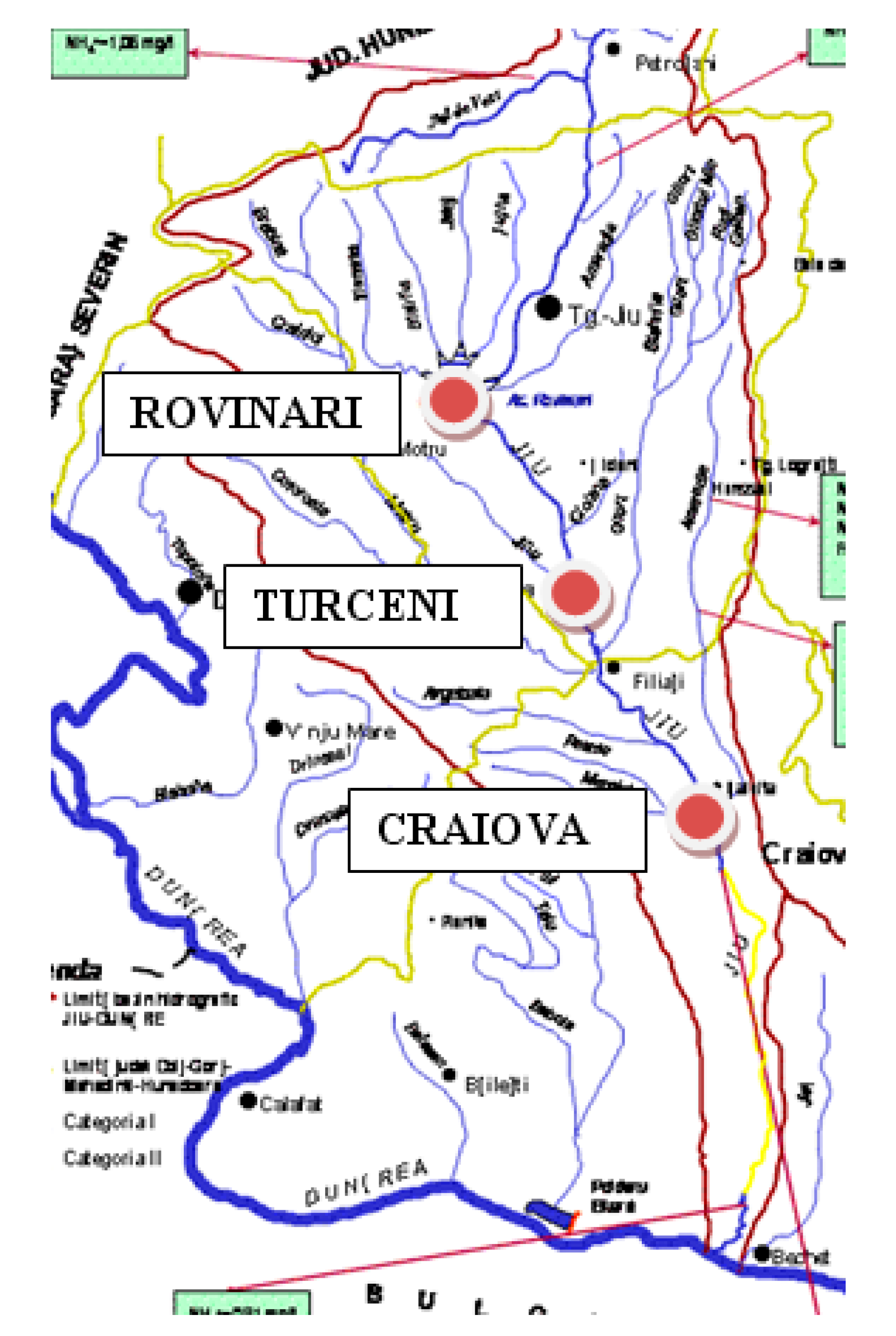
In this study, we take into consideration a chain of three thermoelectric power plants of Romania, namely Rovinari, Turceni and Craiova, situated along Jiu River, into which they are discharging wastewaters (see Figure 1).

Figure 1. Location of Rovinari, Turceni and Craiova thermoelectric power plants along Jiu River in Romania.

Figure 1. Location of Rovinari, Turceni and Craiova thermoelectric power plants along Jiu River in Romania.

The thermoelectric units of the Rovinari, Turceni and Craiova power plants are equipped with a water recirculating system using wet cooling towers in order to dissipate heat from the cooling water to the atmosphere. In this wet recirculating system, the warmed cooling water is pumped from the steam condenser to the cooling towers. However, for economic reasons the power stations are operating as open systems (once-through systems), meaning without recirculation of the water in the cooling system of the power plant. In other words, the necessary fresh water is provided from the river and the wastewater is discharged back to the same river, without using the cooling towers of the power plants.

Taking into consideration the case of three power stations connected in a cascading fashion from the viewpoint of the cooling systems, the wastewaters discharged in the same river could represent a significant environmental impact, concerning aquatic ecosystems in the river. In line with this idea, this paper deals with the assessment of temperature evolution in the river water downstream of the outlet, caused by a warm water discharge. This study reports an evaluation, on the basis of a wastewater thermal pollutant vector, of the environmental impact of wastewater discharged from a chain of power stations into a single river. The wastewater is the spent water used to operate the cooling systems of the power stations.

3. Wastewater Thermal Pollutant Vector of a Chain of Coal-Fired Power Plants along Jiu River

The environmental thermal pollutant vector of wastewaters discharged from Rovinari, Turceni and Craiova coal-fired power plants of Romania are analyzed here. These power stations receive freshwater from and discharge wastewater into the Jiu River [23]. From the viewpoint of the cooling systems, these power plants are connected in a cascading fashion.

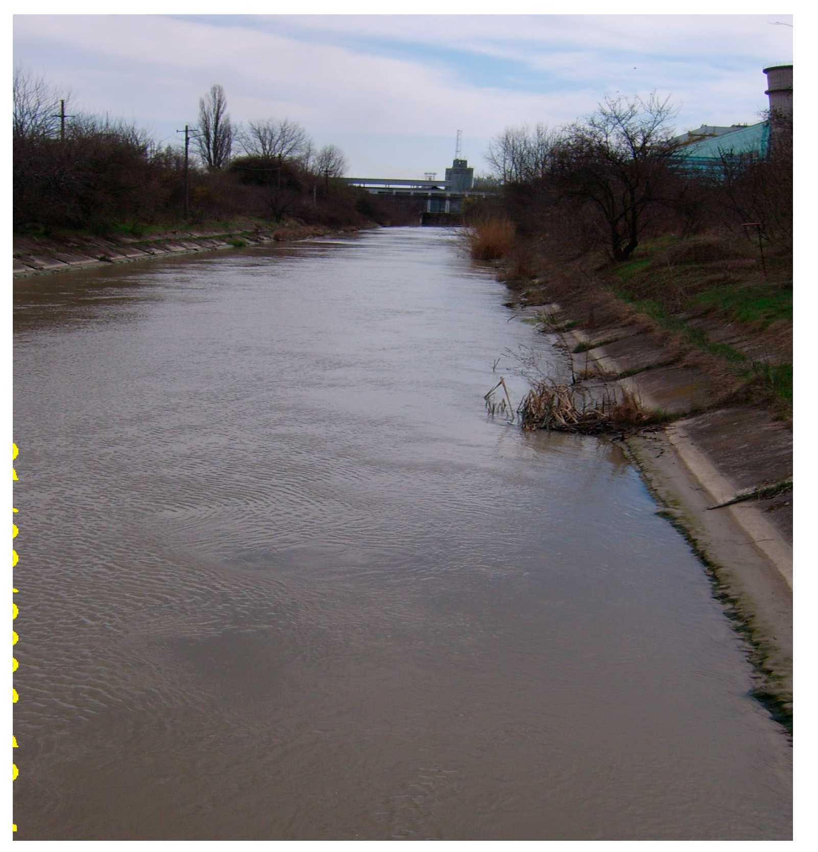
The waters supplied to the thermoelectric units of these power plants are surface waters with a varying temperature (usually in the range 0–30 °C). The pollutant emission source for this river caused by these industrial facilities is mainly associated with the wastewater discharging process. Both the supply of freshwater and the discharge of wastewater are performed through the culvert channels provided with special inlets and outlets, respectively. These surface channels are comprised of concrete and embankment (see Figure 2 and Figure 3), with a slope of 1% to ensure a minimum water flow without destabilizing the optimum level of the natural pond. Figure 2 illustrates the process water culvert channel for the water inlet of the river Jiu. 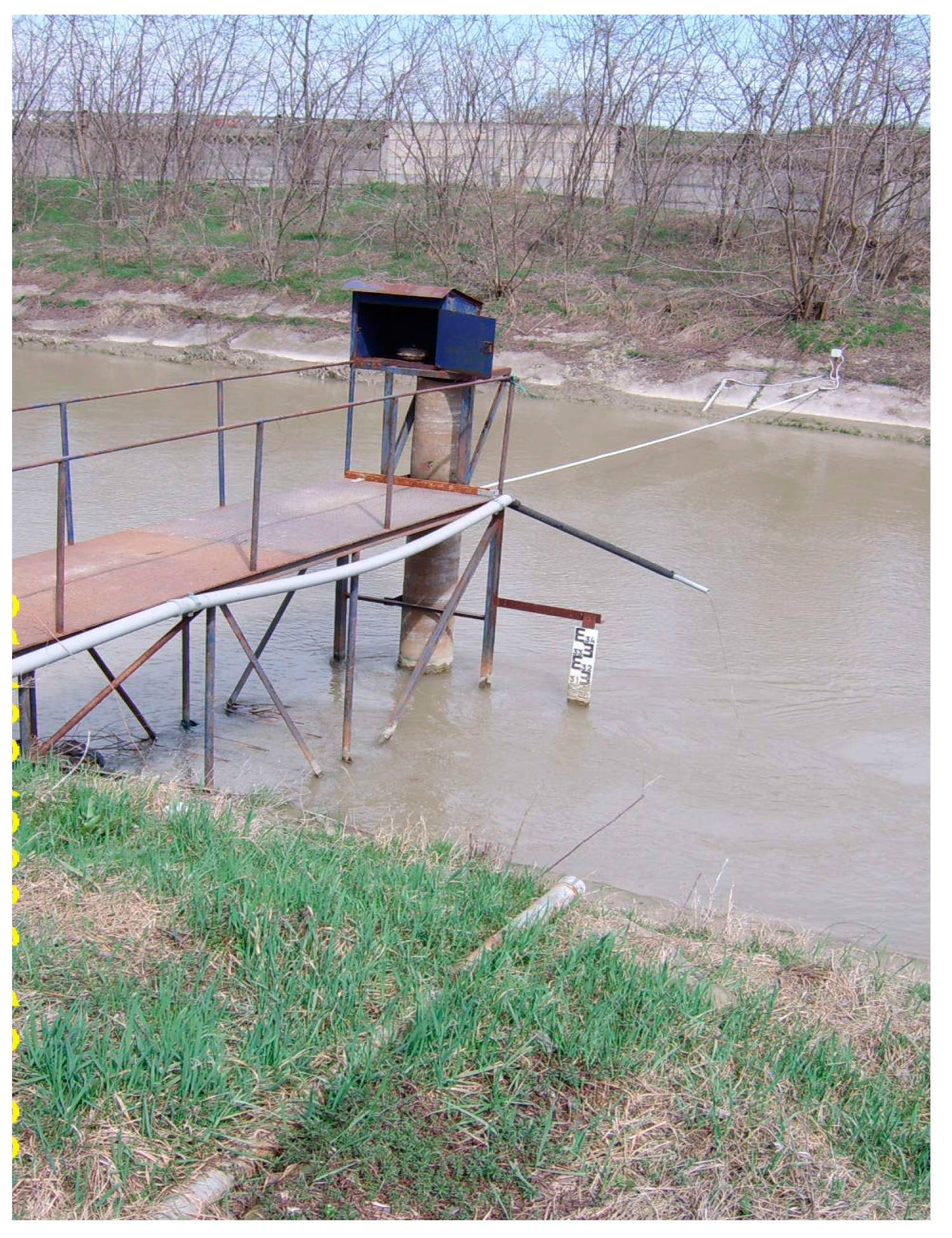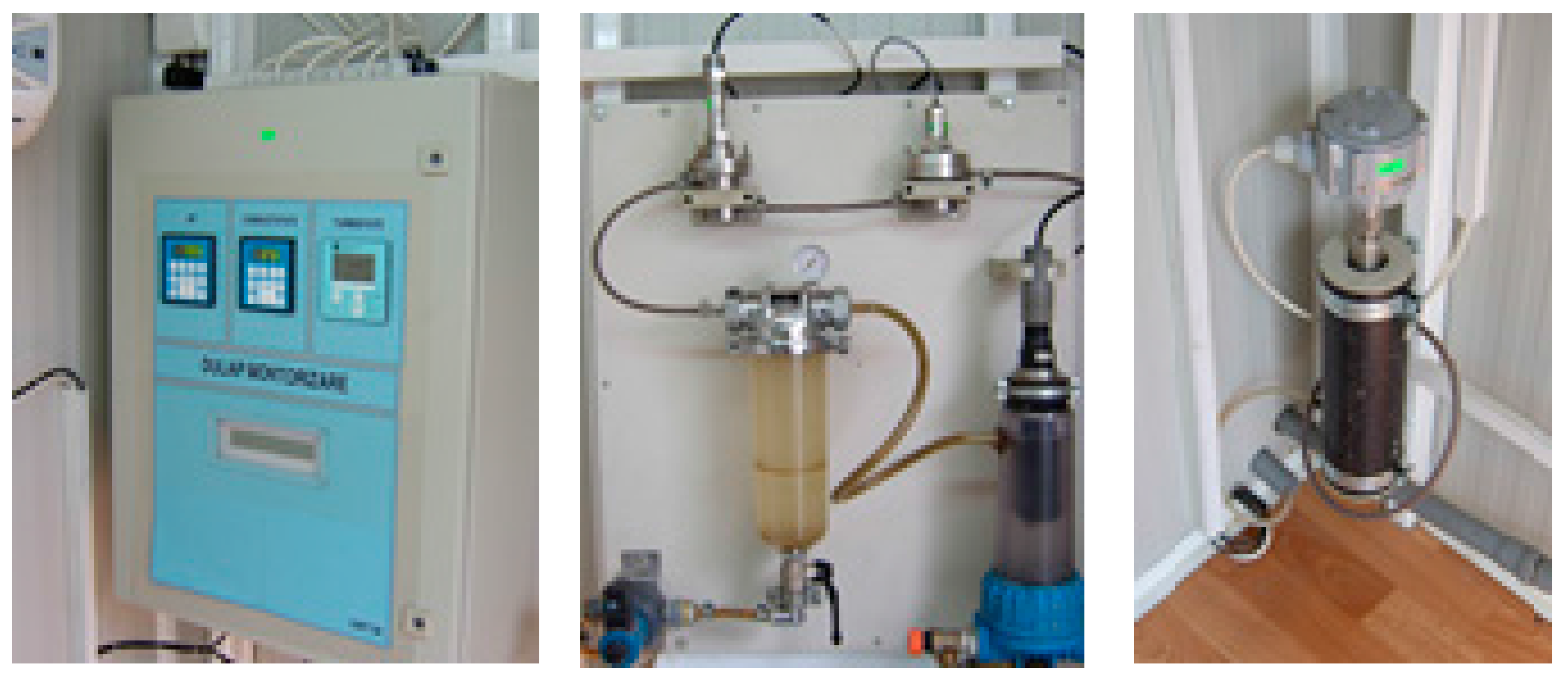Figure 3 shows the technical platform on which is fixed the ultrasonic level sensor. That is the location of the inlet pipe for the test water to be treated in the monitoring cabin, presented in Figure 4.

Figure 2. Longitudinal view of the supply channel.

Figure 2. Longitudinal view of the supply channel.

Figure 3. Experimental platform for supply channel.

Figure 3. Experimental platform for supply channel.

Figure 4. Monitoring cabin.

Figure 4. Monitoring cabin.

The water flow supplied by the Jiu River to these power plants is provided through high capacity pumps and by modifying the upstream dam inlet level. Figure 4 shows the thermostatic and secured cabin for monitoring necessary water parameters, i.e., pH, conductivity, suspensions. The physiochemical parameters are routinely checked, in real time, through complex equipment installed in a monitoring cabin (Figure 4), with a telemetric transmission of the collected data. This way, in the first stage, the following freshwater parameters are determined: conductivity, pH, temperature, water level in the channel, water flow rate, and inlet water flow. The physiochemical parameters of freshwater provided through the supply channel are valuated with the measuring transducers.

Furthermore, water treatment in the Chemical Section is performed to provide the demineralized water necessary for steam production and the softened water to be added in the district heating network.

Water pretreatment is necessary to reduce the suspension in the raw water, using several decanters operating on the basis of coagulation and flocculation processes. Inside the decanters, a decarbonation process also occurs, by treatment with Ca(OH)₂ in order to obtain a precipitation of Ca and Mg soluble salts. Decanted water is stored in tanks, and through a pump system is provided to the demineralized water and softened water installations.

The installation for water demineralizing is necessary to produce an appropriate water for steam production. Water demineralization is carried out through the six units of ionic filters.

The water softening installation provides the softened water to be added to the district heating network.

3.1. Discharged Wastewater Pollutant Vector

The thermoelectric units of the Rovinari, Turceni and Craiova power plants are equipped with a water recirculating system using wet cooling towers in order to dissipate the heat from the cooling water to the atmosphere. In this wet recirculating system, the warmed cooling water is pumped from the steam condenser to the cooling towers [2,8,19,23].

The pollutant vector of discharged wastewater $({\overrightarrow{V}}_{DWW})$ is completely specified (from a strictly vectorial viewpoint) by: direction, sense, magnitude, origin and head-arrow.

The vector direction is defined by the wastewater discharging channel that links the power plant with the river via an ecological wastewater treatment station [23,24,25,26,27,28,29,30,31,32]. The vector sense is defined by the wastewater flowing sense. The vector magnitude is related to the wastewater velocity that must be at minimum 1.5 m/s in order to avoid suspension sedimentation on the discharging channel bottom. The origin of the vector is at the power plant inlet location while the vector head-arrow is at the discharging channel outlet.

The physiochemical parameters of water that can be measured are: temperature, conductivity, particulate matter in suspension, water fixed residue, and pH value. Determination of pH value is necessary to establish the acidic or alkaline nature of the water. Electrometric measurement is a precise method, and the pH-meter has small dimensions and is mobile. Water acidity is associated with the presence of free carbon dioxide, mineral acids and salts of strong acids with weak alkalis. Water alkalinity is associated with the presence of alkaline carbonates, bicarbonates, and hydroxides. This study focuses on the wastewater thermal pollution evaluation.

3.2. Wastewater Thermal Pollutant Vector Plane Projection

The Plane Projection (PP) of wastewater thermal pollutant vector allows for the temperature evaluation in the water flow lane created at certain distances in the river from the wastewater outlet channel. This study deals with long distances (in the range of 1–10 km) on the Jiu River.

Since the simplest method of heat rejection is to discharge the wastewater of a power station cooling system to a river or lake directly, the delineation of thermal discharge should consider the thermal plume that appears at the wastewater outlet in the receiving water [15,16,17,18]. There are many interrelated factors which influence the rate at which thermal plumes disperse and heat is dissipated. The prediction of the size of a thermal plume and its temperature decay are generally made using hydro-physical modeling. The results of such modeling are important to the prediction of the ecological effects, apart from their importance to the operation of a power station. The results of simulations can be useful too, and compared with the results of the experimental measurements of water temperature [15,16,17,18,32,33].

Various approaches [22,33,34] are used to estimate the capacity of water for heat dispersal. This includes mathematical or physical models that have also been developed to predict plume size and dilution behavior.

Whichever methods of plume modeling or measurement are used, knowledge of the detailed temperature patterns and behavior of the thermal plume, particularly of its degree of stability in time and space, are important to ecological impact predictions.

Starting from the above statement, the novelty of this study is that we conceive the method of the wastewater thermal pollutant vector that allows evaluation of the temperature in the water flow path created at certain distances in the river from the wastewater outlet channel.

Basically, the plane projection of the wastewater thermal pollutant vector is related to the water temperature (as a physical parameter). The discharged water can be a surface determined by a complex geometrical figure that can be reduced to an ellipse (point A in the wastewater outlet, and the ellipse center moved in the water flowing sense) [23,30,31,32,33,34]. Our statement is based on the non-uniform river flowing regimes, with a distribution of the flow front stronger in the central axis of the river lane and weaker to the shores (borders). This supports the assumption of the isothermal curves’ modeling pattern of an ellipse type [30,31,32].

An analytical equation of an ellipse with center point O* (x₀, y₀) and semi-axes a and b is:

$$\frac{{(x-x_0)}^2}{a^2}+\frac{{(y-y_0)}^2}{b^2}-1=0$$

(1)

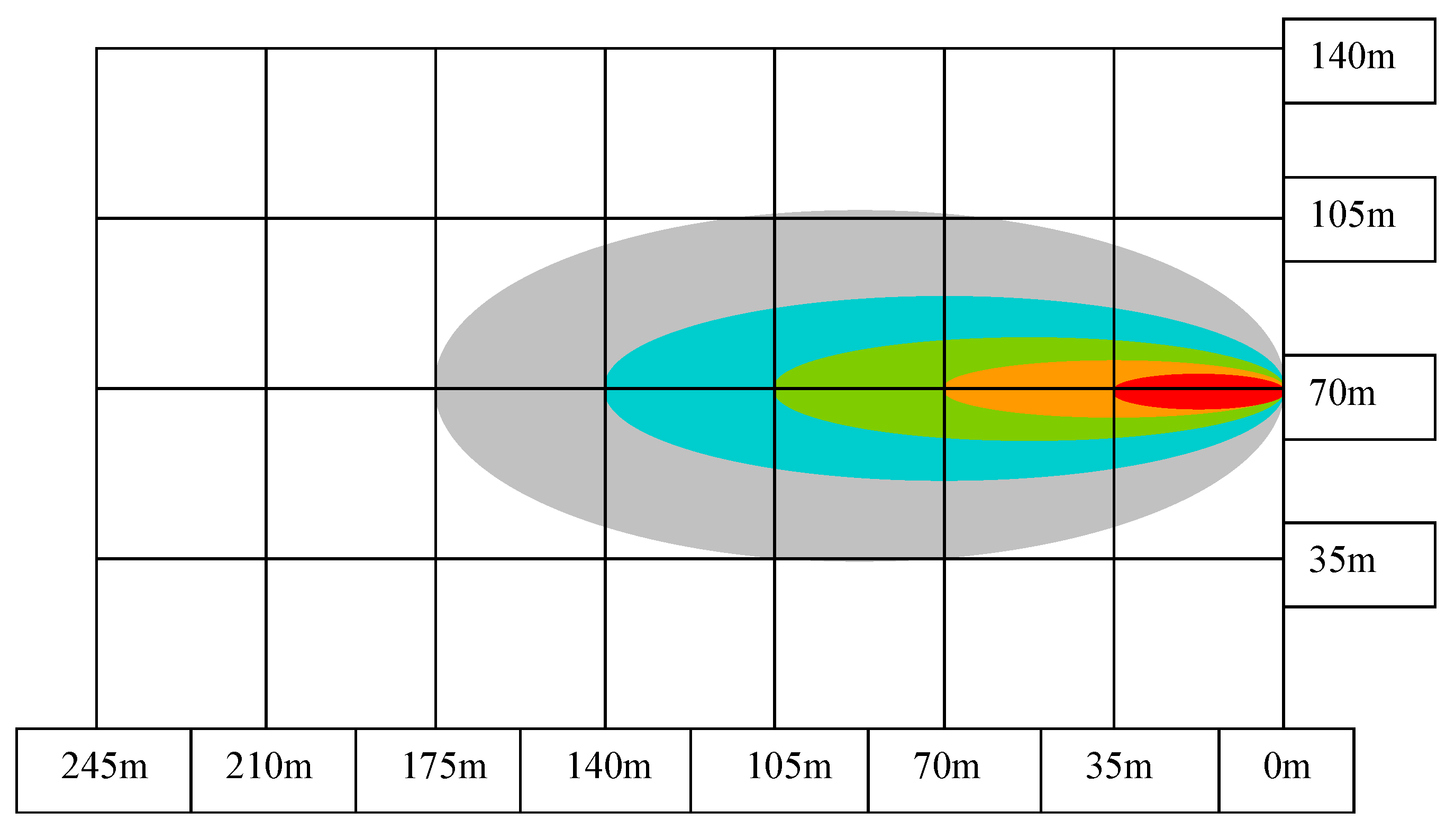
The Plane Projection can be also developed for distances smaller than 250 m. An example of a linear temperature distribution is provided if the Plane Projection can be developed for distances smaller than 250 m inside the main isothermal curve. The distribution of isothermal curves (see Table 1) if the plane projection is on a distance of 175 m in the main flowing lane of wastewater pollutant vector is depicted in Figure 5. In Figure 5, the horizontal and vertical axes of the reference system represent the longitudinal and transversal axes of the ellipse that models the wastewater discharged into the river. The reference system origin (namely, 0 m) corresponds to the power station wastewater outlet. The colours in Table 1 correlate with the colours in Figure 5, which describe the distances on the isothermal curves.

Table 1. Distribution of isothermal curves.

No.	Isothermal Curve	Iso = Isothermal Indicator	Disom [m] = Distance on Isothermal Curve	K [°C/m] = Longitudinal Linearization Coefficient
1	Iso33	33	35	1/35
2	Iso32	32	35	1/35
3	Iso31	31	35	1/35
4	Iso30	30	35	1/35
5	Iso28	29	35	1/35

Table 1. Distribution of isothermal curves.

No.	Isothermal Curve	Iso = Isothermal Indicator	Disom [m] = Distance on Isothermal Curve	K [°C/m] = Longitudinal Linearization Coefficient
1	Iso33	33	35	1/35
2	Iso32	32	35	1/35
3	Iso31	31	35	1/35
4	Iso30	30	35	1/35
5	Iso28	29	35	1/35

Figure 5. Isothermal curves: Iso₃₃, Iso₃₂, Iso₃₁, Iso₃₀, Iso₂₉.

Figure 5. Isothermal curves: Iso₃₃, Iso₃₂, Iso₃₁, Iso₃₀, Iso₂₉.

3.3. The EDF Methodology for Evaluating the Wastewater Thermal Pollutant Vector

From a design viewpoint, the discharged wastewater thermal pollutant vector has as flowing frame of a river laminar layer, variable from the point of the discharging vector outlet. Factors that interfere in the calculation of temperatures within the river, downstream from the outlet discharge point of a warm water flow, are numerous, variable and hard to calculate or measure. This is the reason for applying over time [8,16,17,18,19,23,24,28,29,30,31,32,33,34] an approximate calculus mainly linked to field measurements. The most simple formula does not take into consideration the temperature evolution downstream of the outlet of the wastewater discharging vector, having been concerned only with ensuring the mixture of warm water (from the coal-fired power plant) and the river water does not exceed a limit.

Assessment of temperature evolution in the river water downstream of the outlet, caused by a warm water discharge, is based on a theoretical method consisting of a formula with exponential factors.

Electricity of France (EDF) Group developed a mathematical model of temperature evolution in river water (since a warm water flow had been discharged on downstream by outlets):

$$\text{Δ}t=\mathrm{\Delta }{t}_{\max }\cdot e^{-kx}$$

(2)

where Δt is the river water residual heating x kilometers downstream from the warm water outlet; Δt_max is the river water maximum heating of the water mixture in the warm water outlet; k is a climate correction factor, ranging between 0.001 and 0.01; and x is the distance from the warm water outlet to the river section where the residual temperature is determined.

The mathematic model of temperature evolution in the river water, downstream of the warm water outlet, through the wastewater pollutant vector allows a reliable and accurate evaluation for river lengths of 10 km up to 50 km. Numerical simulation is useful in the technical assessment of transient processes that vary gradually.

3.4. EDF Methodology Applied to Thermoelectric Units of 330 MW of the Rovinari Power Station

This case study takes into consideration operation of the thermoelectric power plant of Rovinari with an installed power corresponding to 3 energetic units (n = 3) of 330 MW, resulting in a total power generation of 990 MW [23,30,31,32]. The investigation aims to assess the evolution of temperature, on the basis of the wastewater pollutant vector. This case study is performed under the following conditions:

• power plant capacity utilization of 75% of the installed power (n = 3);
• the outlet allows the discharge of wastewater provided by the three thermoelectric units of 330 MW;
• temperature assessment is based on the EDF methodology.

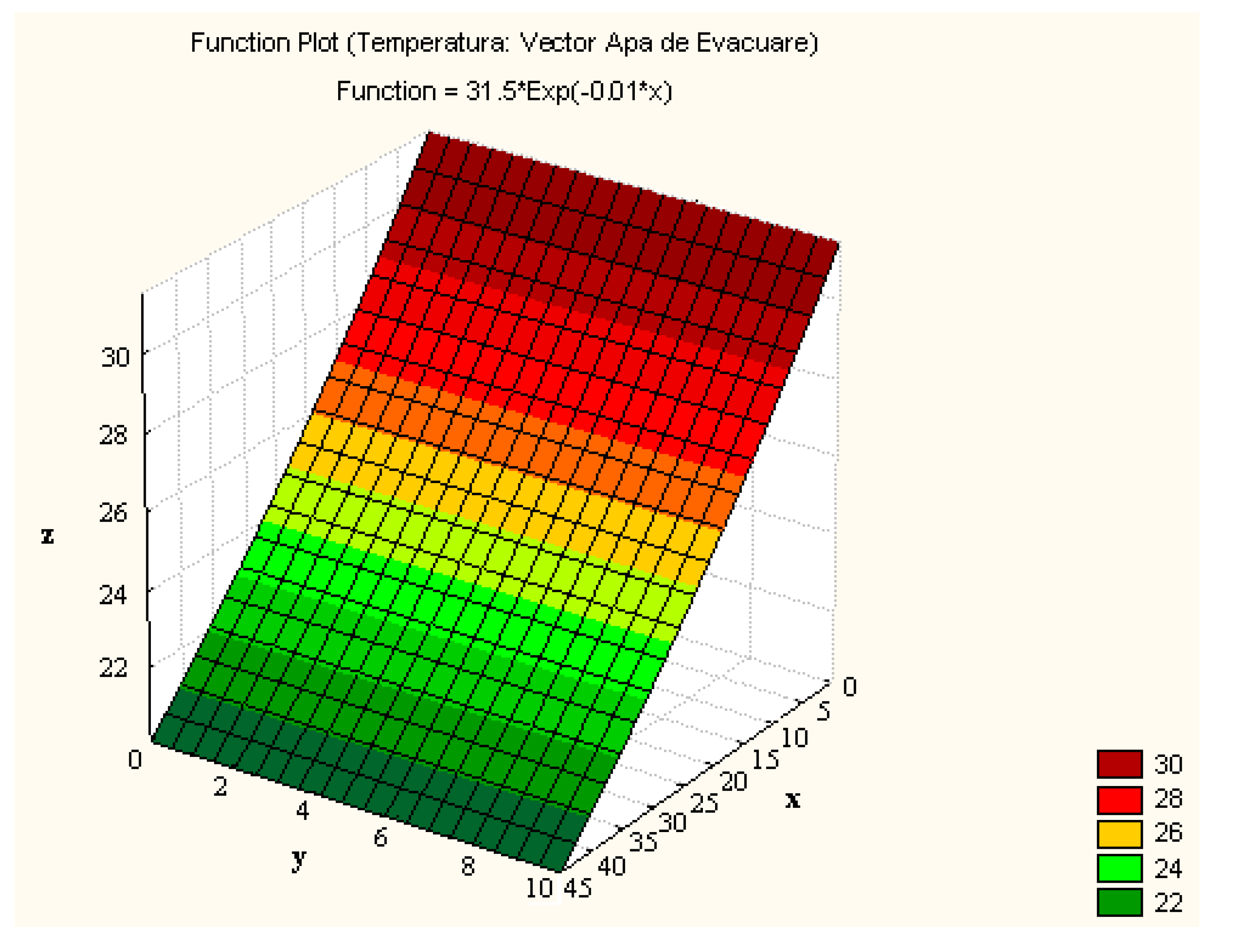
An AMD multiprocessor computer system with StatSoft STATISTICA—Version 7.0 software is used for data acquisition and processing. The simulation process of the EDF pattern for the wastewater thermal pollution vector involves four types of recordings on a 45 km river length, namely:

• temperature nomogram, for k = 0.001 (n = 3), as depicted in Figure 6;
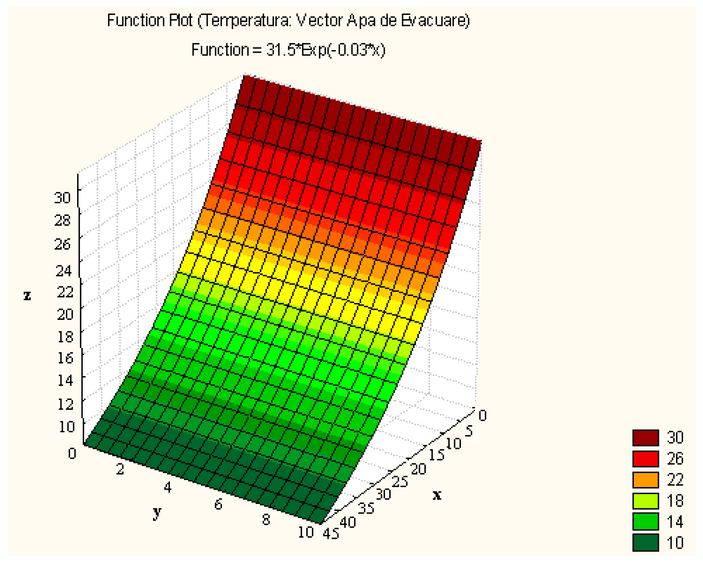
• temperature nomogram, for k = 0.003 (n = 3), as depicted in Figure 7;
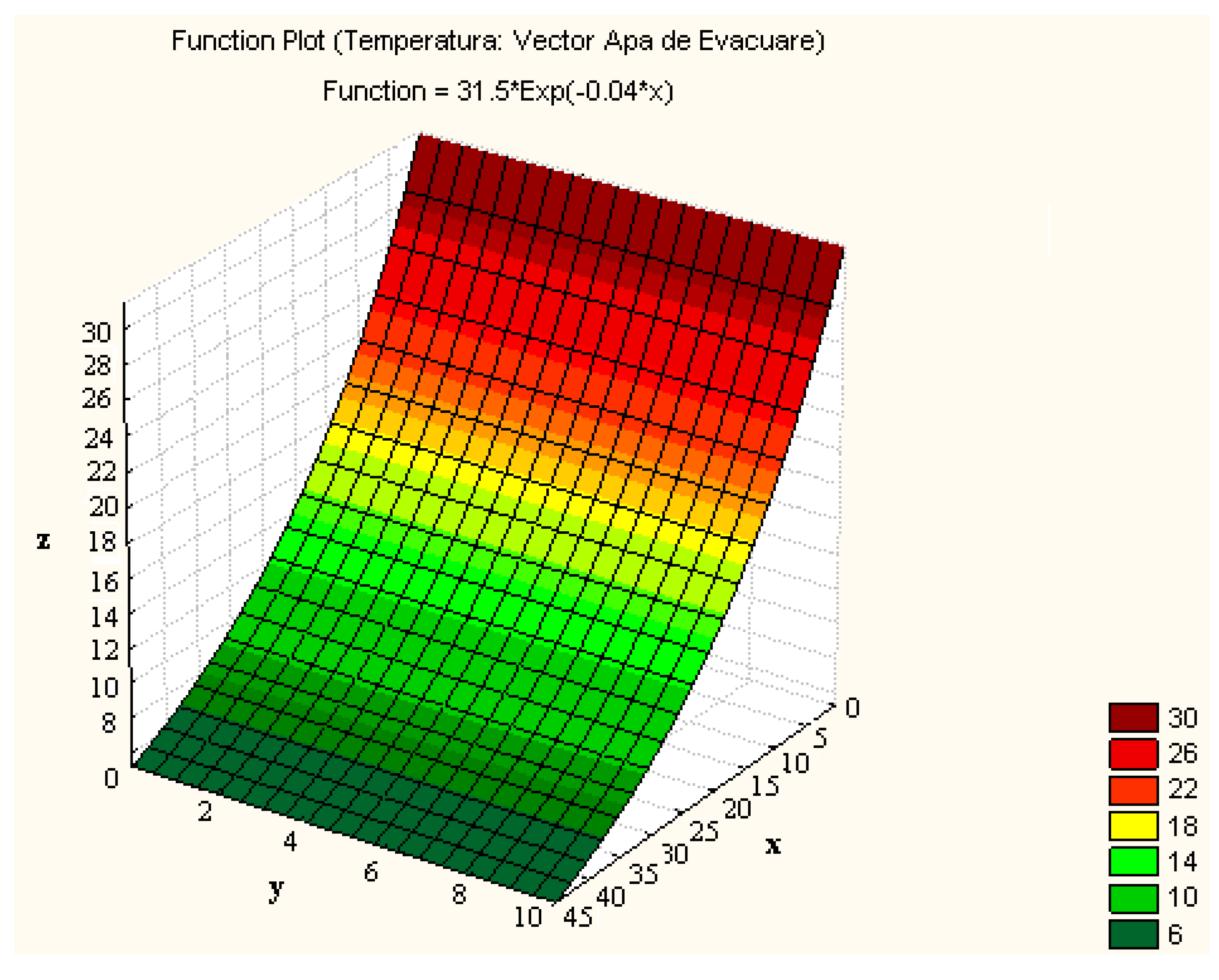
• temperature nomogram, for k = 0.004 (n = 3), as depicted in Figure 8.

Figure 6. Water temperature nomogram for k = 0.001 (n = 3).

Figure 6. Water temperature nomogram for k = 0.001 (n = 3).

Figure 7. Water temperature nomogram for k = 0.003 (n = 3).

Figure 7. Water temperature nomogram for k = 0.003 (n = 3).

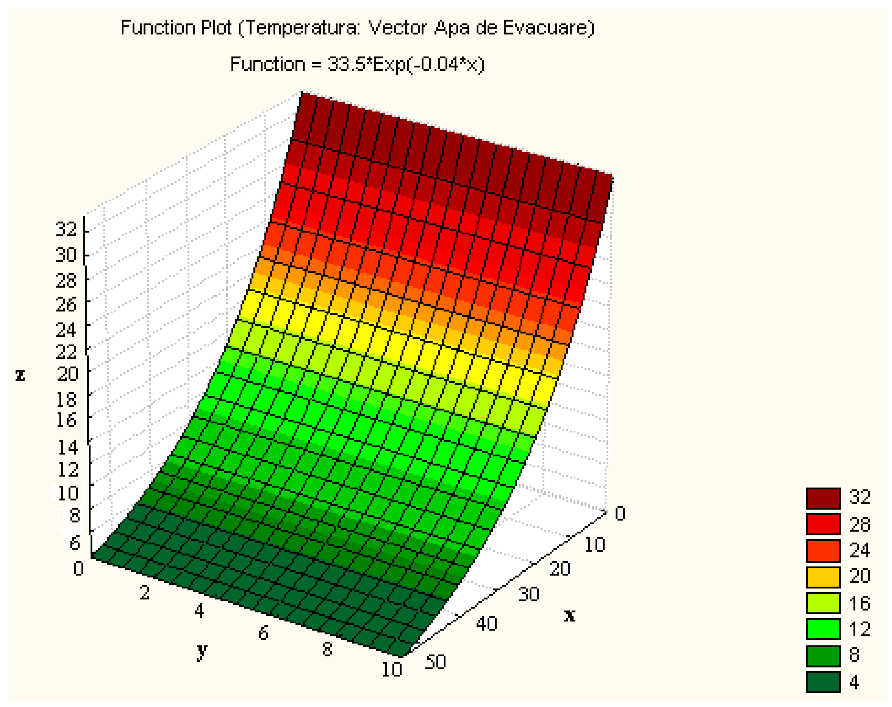
Figure 8. Water temperature nomogram for k = 0.004 (n = 3).

Figure 8. Water temperature nomogram for k = 0.004 (n = 3).

Note in Figure 6, Figure 7 and Figure 8 that the simulations have two variables:

• variable x, which represents the distance from the river outlet point of warm wastewater to the river section where the residual heating is calculated;
• variable y, denoted by k and representing the climate correction factor, with values ranging between 0.001 and 0.01.

The mathematical pattern response to the simulation is represented by the multivariable function z denoted by Δt (river water residual heating at x kilometers from the warm water discharging outlet). The red colour indicates high values of temperature, obtained in the wastewater outlet.

It is emphasized in the mathematical model that the parameter Δt_m represents the maximum heating of river water after mixing with the warm water outlet.

3.5. Experimental Validation of EDF Methodology Results on Thermoelectric Units of 330 MW of Rovinari Power Stations

Under the above mentioned conditions, for an acceptable evaluation of the mathematical pattern described by the EDF formula, it is necessary to join the simulations with experimental tests. For the experimental validation of the EDF model, on Jiu River have been performed recordings both for natural thermal load (JIU STN) on the upstream river and for the Rovinari thermal load (JIU STR) on river downstream. These data were obtained with the support of the Rovinari Power Plant staff. 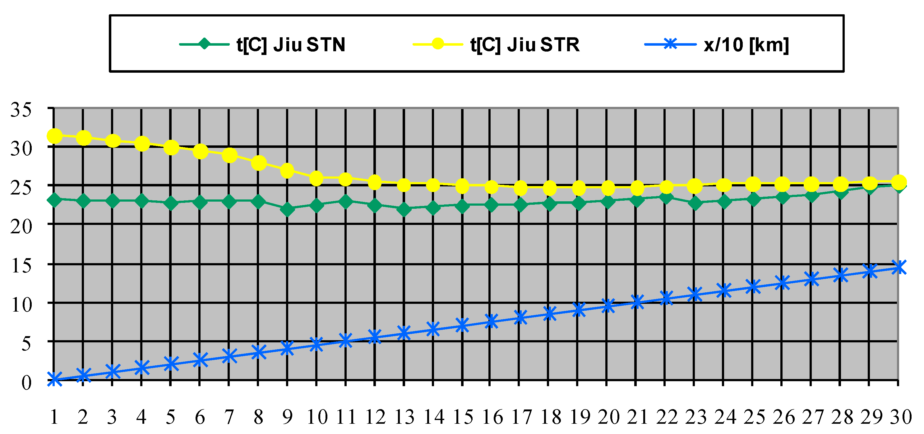Table 2 and Figure 9 show the temperature evolution along the river length. In Table 2, we indicate with red bold font the river water temperature at the wastewater outlet of the Rovinari power plant.

Table 2. Temperature t and distance x data series for Jiu River STN and Jiu River STR.

t [C]	t [C]	x	Reading
Jiu River STN	Jiu River STR	[km]	Number
23.2	31.5	0.0	1
23.1	31.2	0.5	2
23.1	30.8	1.0	3
23.1	30.5	1.5	4
22.8	30.0	2.0	5
22.9	29.5	2.5	6
23.0	29.0	3.0	7
23.0	28.0	3.5	8
22.0	27.0	4.0	9
22.5	26.0	4.5	10
23.0	25.9	5.0	11
22.5	25.5	5.5	12
22.0	25.1	6.0	13
22.2	25.1	6.5	14
22.4	25.0	7.0	15
22.6	24.9	7.5	16
22.6	24.8	8.0	17
22.7	24.8	8.5	18
22.8	24.7	9.0	19
23.0	24.7	9.5	20
23.2	24.8	10.0	21
23.6	24.9	10.5	22
22.8	25.0	11.0	23
23.0	25.1	11.5	24
23.3	25.2	12.0	25
23.6	25.2	12.5	26
23.8	25.3	13.0	27
24.2	25.3	13.5	28
24.8	25.4	14.0	29
25.0	25.5	14.5	30

Table 2. Temperature t and distance x data series for Jiu River STN and Jiu River STR.

t [C]	t [C]	x	Reading
Jiu River STN	Jiu River STR	[km]	Number
23.2	31.5	0.0	1
23.1	31.2	0.5	2
23.1	30.8	1.0	3
23.1	30.5	1.5	4
22.8	30.0	2.0	5
22.9	29.5	2.5	6
23.0	29.0	3.0	7
23.0	28.0	3.5	8
22.0	27.0	4.0	9
22.5	26.0	4.5	10
23.0	25.9	5.0	11
22.5	25.5	5.5	12
22.0	25.1	6.0	13
22.2	25.1	6.5	14
22.4	25.0	7.0	15
22.6	24.9	7.5	16
22.6	24.8	8.0	17
22.7	24.8	8.5	18
22.8	24.7	9.0	19
23.0	24.7	9.5	20
23.2	24.8	10.0	21
23.6	24.9	10.5	22
22.8	25.0	11.0	23
23.0	25.1	11.5	24
23.3	25.2	12.0	25
23.6	25.2	12.5	26
23.8	25.3	13.0	27
24.2	25.3	13.5	28
24.8	25.4	14.0	29
25.0	25.5	14.5	30

Normally, the medium river flow rate at the Rovinari site is roughly 47 m³/s [23,24,25]. The operation of three thermoelectric units in open circuit of the Rovinari power plant relies on this river flow, under the stability conditions for the relevant environmental parameters.

The measurement conditions assume the following:

(1)

Maintaining in operation three thermoelectric units of 330 MW in Rovinari for 5 h (4 h before measurement and 1 h during measuring).

(2)

Positioning a human observer with a measuring instrument (precision digital thermometer) along the riverbed and in the mainstream of the river, at intervals of 5 km.

(3)

Establishing the trigger timing of the readings, chosen to be 10 AM, since according to legislation [21], this is the most appropriate time from the viewpoint of heat exchange between Jiu River and the environmental surroundings.

(4)

Performing the 11 temperature readings, over a period of 50 min, at intervals of 5 min.

Figure 9. Diagram of t and x data series for Jiu River STN and Jiu River STR.

Figure 9. Diagram of t and x data series for Jiu River STN and Jiu River STR.

An AMD multiprocessor computer system with Microsoft Office—Version 7.0 software is used for data acquisition and processing.

The experimental validation of the EDF pattern for the wastewater thermal pollutant vector in this case study is shown in Figure 9, which shows data for temperature t [°C] and distance x [km] on River Jiu, for the natural thermal load (Jiu River STN) and for the Rovinari thermal load (Jiu River STR).

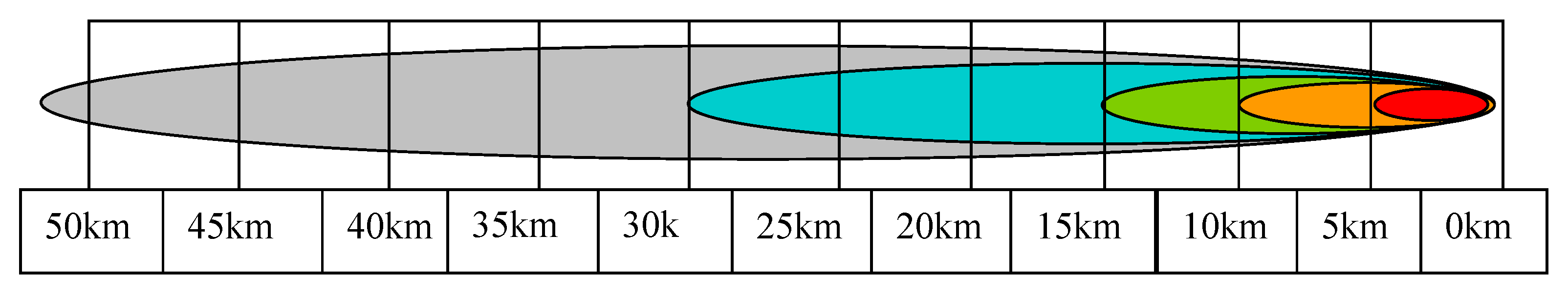
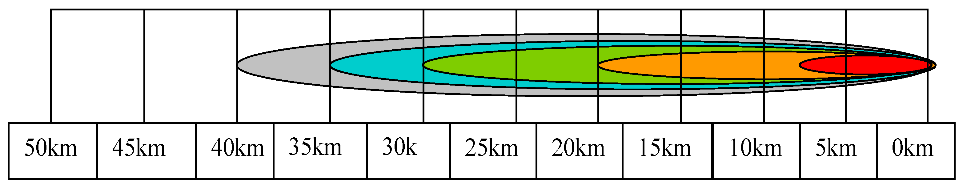
In Table 3 and Figure 10, the isothermal curves Iso₃₁, Iso₃₀, Iso₂₉, Iso₂₈, Iso₂₇ are depicted.

Table 3. Data of isothermal curves Iso₃₁, Iso₃₀, Iso₂₉, Iso₂₈, Iso₂₇.

No.	Isothermal Curve	Iso = Isothermal Indicator	Δtm [°C] = Outlet Water Temperature	k [km−1] = Correction Factor
1	Iso31	31	31.5	0.004
2	Iso30	30	31.5	0.004
3	Iso29	29	31.5	0.004
4	Iso28	28	31.5	0.004
5	Iso27	27	31.5	0.004

Table 3. Data of isothermal curves Iso₃₁, Iso₃₀, Iso₂₉, Iso₂₈, Iso₂₇.

No.	Isothermal Curve	Iso = Isothermal Indicator	Δtm [°C] = Outlet Water Temperature	k [km−1] = Correction Factor
1	Iso31	31	31.5	0.004
2	Iso30	30	31.5	0.004
3	Iso29	29	31.5	0.004
4	Iso28	28	31.5	0.004
5	Iso27	27	31.5	0.004

Figure 10. Isothermal curves: Iso₃₁, Iso₃₀, Iso₂₉, Iso₂₈, Iso₂₇.

Figure 10. Isothermal curves: Iso₃₁, Iso₃₀, Iso₂₉, Iso₂₈, Iso₂₇.

The colours in Table 3 correlate with the colours in Figure 10, which describe the distances on the isothermal curves.

Accordingly, it can be observed that:

• the limit x = 7.5 km for the isothermal curve Iso₃₁ = 31 °C;
• the limit x = 20 km for the isothermal curve Iso₃₀ = 30 °C;
• the limit x = 30 km for the isothermal curve Iso₂₉ = 29 °C;
• the limit x = 35 km for the isothermal curve Iso₂₈ = 28 °C;
• the limit x = 40 km for the isothermal curve Iso₂₇ = 27 °C.

Consequently:

• for k = 0.003 km⁻¹, Δt_max = 31.5 °C, n = 3, P_inst/unit = 330 MW, P_inst = 990 MW, the maximum relative error is ε_rel ≤ 5.85%;
• for k = 0.004 km⁻¹, Δt_max = 31.5 °C, n = 3, P_inst/unit = 330 MW, P_inst = 990 MW, the maximum relative error is ε_rel ≤ 3.66%;
• for k = 0.005 km⁻¹, Δt_max = 31.5 °C, n = 3, P_inst/unit = 330 MW, P_inst = 990 MW, the maximum relative error is ε_rel ≤ 6.51%;
• the optimum of the mathematical model according to relative error, under the conditions Δt_max= 31.5 °C, n = 3, P_inst/unit = 330 MW and P_inst = 990 MW, is given by k = 0.004 km⁻¹.

3.6. EDF Methodology Applied to Thermoelectric Units of 330 MW of Rovinari and Turceni Power Stations in Simultaneous Operation

Now, this case study takes into consideration the continuous operation of the thermoelectric power plant of Rovinari with a power corresponding to three energetic units (n = 3) of 330 MW (resulting in a total power of 990 MW, which represents 75% of the total installed power) plus the continuous operation of the coal-fired power plant of Turceni with a power corresponding to three energetic units (n = 3) of 330 MW (resulting the total power of 990 MW, which represents 50% of the total installed power) [26,27,28].

Figure 11. Water temperature nomogram for k = 0.004 (n = 6).

Figure 11. Water temperature nomogram for k = 0.004 (n = 6).

The wastewater thermal pollutant vector investigation aims to assess the correct evolution of temperature, on the basis of the EDF Methodology.

Note in this case that the outlets allow the discharge of wastewater provided by three thermoelectric units of 330 MW from the Rovinari power plant and three thermoelectric units of 330 MW from the Turceni power plant.

Following the same procedure as before, the simulation process of the EDF pattern for the wastewater pollution vector involves four types of recording on a 45 km river length, namely:

• temperature nomogram, k = 0.004 (n = 6), depicted by Figure 11, as an example;
• temperature nomogram, k = 0.0054 (n = 6);
• temperature nomogram, k = 0.006 (n = 6).

3.7. Experimental Validation of EDF Methodology Results on Thermoelectric Units of 330 MW of Rovinari and Turceni Power Stations in Simultaneous Operation

To provide experimental validation of the EDF model, in Jiu River, readings are taken [30,31,32] both for natural thermal load (JIU STN) in the upstream river and for the Rovinari and Turceni thermal loads (JIU STRT) in the downstream river for Turceni.

Normally, the medium river flow rate at the Rovinari site is roughly 47 m³/s, and at the Turceni site is roughly 54.5 m³/s. Operation of three thermoelectric units, in open circuit of the Rovinari and Turceni power plants relies on these river flow rates, under the stability conditions for the relevant environmental parameters.

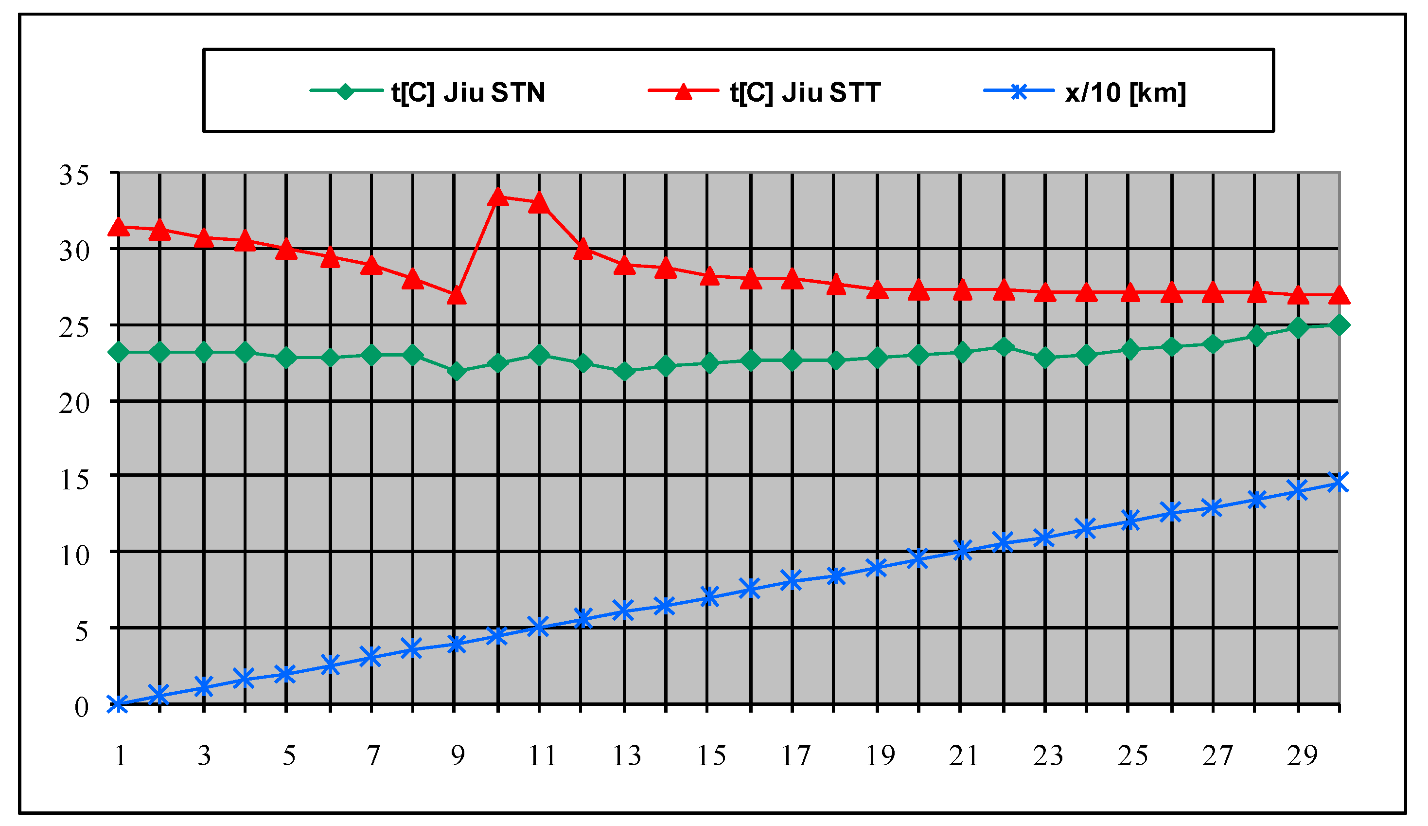
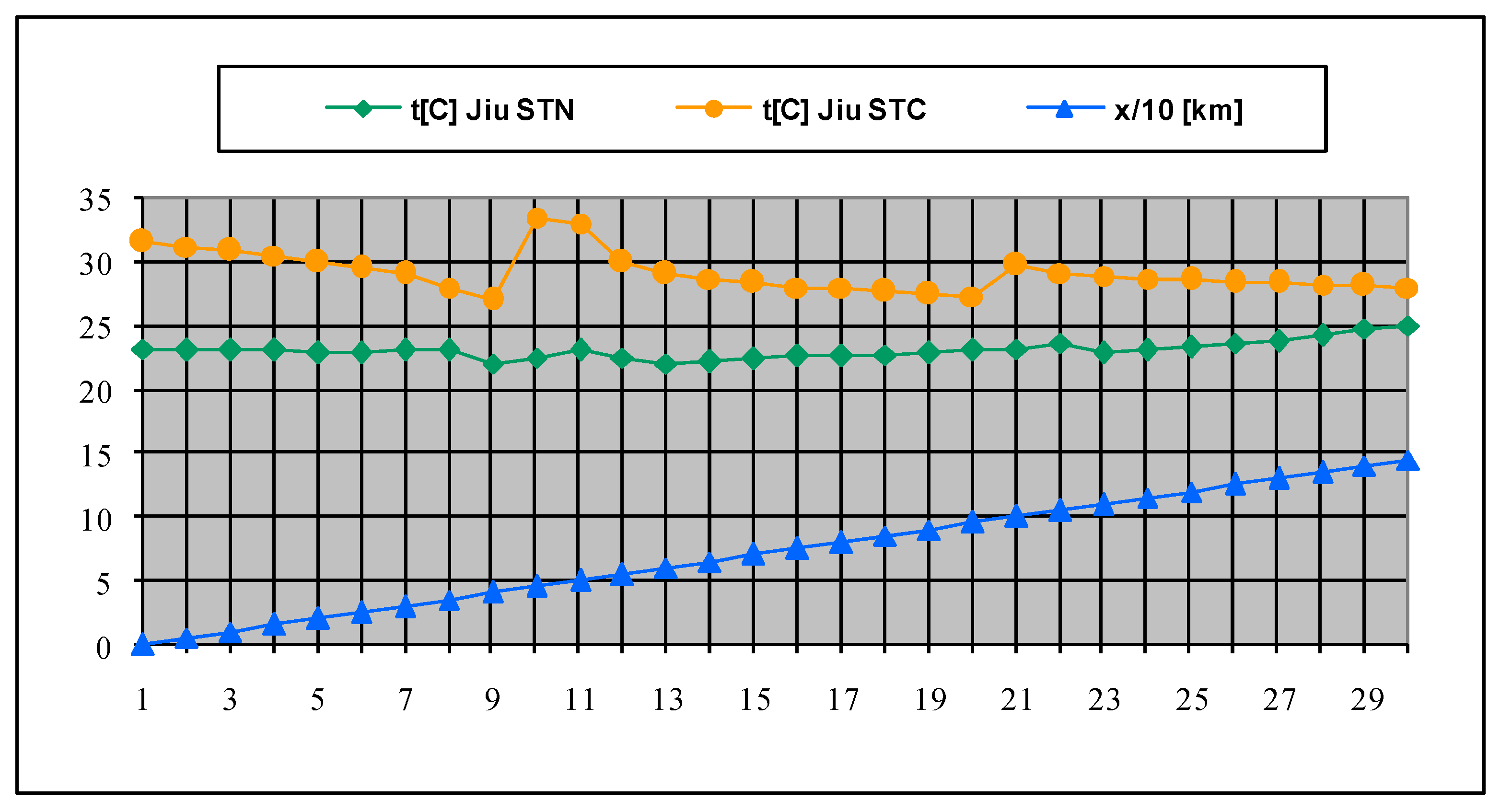
Under the same measurement conditions as before, the experimental validation of the EDF pattern for the wastewater thermal pollutant vector in this case study is shown in Table 4 and Figure 12, which depict the temperature t [°C] and distance x [km] on River Jiu for natural thermal load (Jiu River STN) and for the Rovinari and Turceni thermal loads (Jiu River STRT). In Table 4, we indicate with red bold font the river water temperature points at the wastewater outlets of the Rovinari and Turceni power plants. 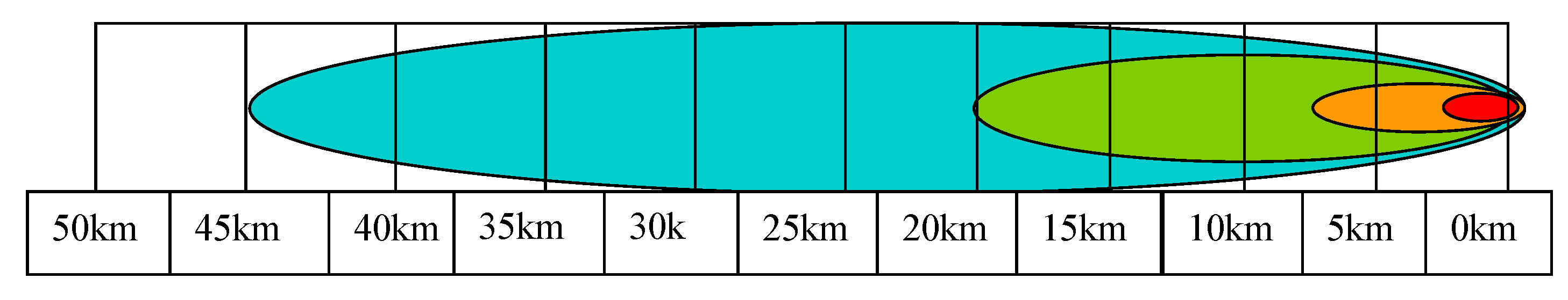In Figure 13, the isothermal curves Iso₃₃, Iso₃₀, Iso₂₉, Iso₂₈, Iso₂₇ are depicted.

Figure 12. Diagram of t and x data series for Jiu River STN and Jiu River STRT.

Figure 12. Diagram of t and x data series for Jiu River STN and Jiu River STRT.

Figure 13. Isothermal curves: Iso₃₃, Iso₃₀, Iso₂₉, Iso₂₈, Iso₂₇.

Figure 13. Isothermal curves: Iso₃₃, Iso₃₀, Iso₂₉, Iso₂₈, Iso₂₇.

Table 4. Temperature t and distance x data series for Jiu River STN and Jiu River STRT.

t [C]	t [C]	x/10	Reading
Jiu STN	Jiu STRT	[km]	Number
23.2	31.5	0.0	1
23.1	31.2	0.5	2
23.1	30.8	1.0	3
23.1	30.5	1.5	4
22.8	30.0	2.0	5
22.9	29.5	2.5	6
23.0	29.0	3.0	7
23.0	28.0	3.5	8
22.0	27.0	4.0	9
22.5	33.5	4.5	10
23.0	33.0	5.0	11
22.5	30.0	5.5	12
22.0	29.0	6.0	13
22.2	28.7	6.5	14
22.4	28.3	7.0	15
22.6	28.0	7.5	16
22.6	28.0	8.0	17
22.7	27.7	8.5	18
22.8	27.4	9,0	19
23.0	27.3	9.5	20
23.2	27.3	10.0	21
23.6	27.3	10.5	22
22.8	27.2	11.0	23
23.0	27.2	11.5	24
23.3	27.2	12.0	25
23.6	27.1	12.5	26
23.8	27.1	13.0	27
24.2	27.1	13.5	28
24.8	27.0	14.0	29
25.0	27.0	14.5	30

Table 4. Temperature t and distance x data series for Jiu River STN and Jiu River STRT.

t [C]	t [C]	x/10	Reading
Jiu STN	Jiu STRT	[km]	Number
23.2	31.5	0.0	1
23.1	31.2	0.5	2
23.1	30.8	1.0	3
23.1	30.5	1.5	4
22.8	30.0	2.0	5
22.9	29.5	2.5	6
23.0	29.0	3.0	7
23.0	28.0	3.5	8
22.0	27.0	4.0	9
22.5	33.5	4.5	10
23.0	33.0	5.0	11
22.5	30.0	5.5	12
22.0	29.0	6.0	13
22.2	28.7	6.5	14
22.4	28.3	7.0	15
22.6	28.0	7.5	16
22.6	28.0	8.0	17
22.7	27.7	8.5	18
22.8	27.4	9,0	19
23.0	27.3	9.5	20
23.2	27.3	10.0	21
23.6	27.3	10.5	22
22.8	27.2	11.0	23
23.0	27.2	11.5	24
23.3	27.2	12.0	25
23.6	27.1	12.5	26
23.8	27.1	13.0	27
24.2	27.1	13.5	28
24.8	27.0	14.0	29
25.0	27.0	14.5	30

According to the data depicted above, it can be observed that:

• the limit x = 5 km for the isothermal curve Iso₃₃ = 33 °C;
• the limit x = 10 km for the isothermal curve Iso₃₀ = 30 °C;
• the limit x = 15 km for the isothermal curve Iso₂₉ = 29 °C;
• the limit x = 30 km for the isothermal curve Iso₂₈ = 28 °C;
• the limit x = 52.5 km for the isothermal curve Iso₂₇ = 27 °C.

Consequently:

• for k = 0.004 km⁻¹, Δt_max = 31.5 °C, n = 6, P_inst/unit = 330 MW, P_inst = 1980 MW, the maximum relative error is ε_rel ≤ 8.79%;
• for k = 0.0054 km⁻¹, Δt_max = 31.5 °C, n = 6, P_inst/unit = 330 MW, P_inst = 1980 MW, the maximum relative error is ε_rel ≤ 6.53%;
• for k = 0.006 km⁻¹, Δt_max = 31.5 °C, n = 6, P_inst/unit = 330 MW, P_inst = 1980 MW, the maximum relative error is ε_rel ≤ 9.09%.
• the optimum of the mathematical model according to relative error, under the conditions Δt_max = 31.5 °C, n = 6, P_inst/unit = 330 MW, P_inst = 1980 MW, is given by k = 0.0054 km⁻¹.

3.8. EDF Methodology Applied to Thermoelectric Units of 330 MW of Rovinari, Turceni and Craiova Power Stations in Simultaneous Operation

The third situation in this case study considers the continuous, simultaneous operation of three coal-fired power plants which are connected in a cascade manner, from the cooling system viewpoint, since they are supplying freshwater from and discharged wastewater in the Jiu River. This case study is performed under the following conditions:

• the Rovinari power plant operates with three units of 330 MW (capacity utilization of 75% of the installed power);
• the Turceni power plant operates with three units of 330 MW (capacity utilization of 50% of the installed power);
• the Craiova power plant operates with three units of 330 MW (capacity utilization of 100% of the installed power);
• the total installed power is 2970 MW;
• the outlets of these power plants allow the discharge of wastewater provided by the nine thermoelectric blocks of 330 MW, comprised of three units from each power plant;
• temperature assessment is based on the EDF methodology.

Following the same procedure, the simulation process of the EDF pattern for the wastewater pollution vector involves four types of recordings on a 45 km river length, namely:

• temperature nomogram, k = 0.001 (n = 9), depicted by Figure 14, as an example;
• temperature nomogram, k = 0.002 (n = 9);
• temperature nomogram, k = 0.003 (n = 9).

Figure 14. Water temperature nomogram for k = 0.001 (n = 9).

Figure 14. Water temperature nomogram for k = 0.001 (n = 9).

3.9. Experimental Validation of EDF Methodology Results of Thermoelectric Units of 330 MW of Rovinari, Turceni and Craiova Power Stations in Simultaneous Operation

To provide experimental validation of the EDF model, on Jiu River readings are taken both for the natural thermal load (JIU STN) on the river upstream, and for the Rovinari and Turceni and Craiova thermal loads (JIU STRTC) on the downstream river in Craiova [29,30,31,32].

Normally, the medium river flow at the Rovinari site is roughly 47 m³/s, while at the Turceni site it is roughly 54.5 m³/s and at the Craiova site it is roughly 80 m³/s.

The experimental validation of the EDF pattern for the wastewater pollutant vector in this case study is illustrated in Table 5 and Figure 15. That diagram depicts the temperature t [°C] and distance x [km] on River Jiu, for the natural thermal load (Jiu River STN) and for the Rovinari + Turceni + Craiova thermal loads (Jiu River STRTC). In Table 5, we indicate with red bold fonts the river water temperature points at the wastewater outlets of the Rovinari, Turceni and Craiova power plants. In Figure 16, the isothermal curves Iso_29.5, Iso₂₉, Iso_28.5, Iso₂₈ are shown.

Table 5. Temperature t and distance x data series for Jiu River STN and Jiu River STRTC.

t [C]	t [C]	x/10	Reading
Jiu STN	Jiu STRTC	[km]	Number
23.2	31.5	0.0	1
23.1	31.2	0.5	2
23.1	30.8	1.0	3
23.1	30.5	1.5	4
22.8	30.0	2.0	5
22.9	29.5	2.5	6
23.0	29.0	3.0	7
23.0	28.0	3.5	8
22.0	27.0	4.0	9
22.5	33.5	4.5	10
23.0	33.0	5.0	11
22.5	30.0	5.5	12
22.0	29.0	6.0	13
22.2	28.7	6.5	14
22.4	28.3	7.0	15
22.6	28.0	7,5	16
22.6	28.0	8.0	17
22.7	27.7	8.5	18
22.8	27.4	9.0	19
23.0	27.3	9.5	20
23.2	29.7	10.0	21
23.6	29.1	10.5	22
22.8	28.9	11.0	23
23.0	28.7	11,5	24
23.3	28.5	12.0	25
23,6	28.4	12.5	26
23.8	28.3	13.0	27
24.2	28.2	13.5	28
24,8	28.1	14.0	29
25.0	28.0	14.5	30

Table 5. Temperature t and distance x data series for Jiu River STN and Jiu River STRTC.

t [C]	t [C]	x/10	Reading
Jiu STN	Jiu STRTC	[km]	Number
23.2	31.5	0.0	1
23.1	31.2	0.5	2
23.1	30.8	1.0	3
23.1	30.5	1.5	4
22.8	30.0	2.0	5
22.9	29.5	2.5	6
23.0	29.0	3.0	7
23.0	28.0	3.5	8
22.0	27.0	4.0	9
22.5	33.5	4.5	10
23.0	33.0	5.0	11
22.5	30.0	5.5	12
22.0	29.0	6.0	13
22.2	28.7	6.5	14
22.4	28.3	7.0	15
22.6	28.0	7,5	16
22.6	28.0	8.0	17
22.7	27.7	8.5	18
22.8	27.4	9.0	19
23.0	27.3	9.5	20
23.2	29.7	10.0	21
23.6	29.1	10.5	22
22.8	28.9	11.0	23
23.0	28.7	11,5	24
23.3	28.5	12.0	25
23,6	28.4	12.5	26
23.8	28.3	13.0	27
24.2	28.2	13.5	28
24,8	28.1	14.0	29
25.0	28.0	14.5	30

Figure 15. Diagram of t and x data series for Jiu River STN and Jiu River STRTC.

Figure 15. Diagram of t and x data series for Jiu River STN and Jiu River STRTC.

Figure 16. Isothermal curves: Iso_29.5, Iso₂₉, Iso_28.5, Iso₂₈.

Figure 16. Isothermal curves: Iso_29.5, Iso₂₉, Iso_28.5, Iso₂₈.

Accordingly, it can be observed that:

• the limit x = 2.5 km for the isothermal curve Iso_29.5 = 29.5 °C;
• the limit x = 7.5 km for the isothermal curve Iso₂₉ = 29 °C;
• the limit x = 20 km for the isothermal curve Iso_28.5 = 28.5 °C;
• the limit x = 45 km for the isothermal curve Iso₂₈ = 28 °C.

Consequently:

• for k = 0.001 km⁻¹, Δt_max = 29.7 °C, n = 9, P_inst/unit = 330 MW, P_inst = 2970 MW, the maximum relative error is ε_rel ≤ 2.15%;
• for k = 0.002 km⁻¹, Δt_max = 29.7 °C, n = 9, P_inst/unit = 330 MW, P_inst = 2970 MW, the maximum relative error is ε_rel ≤ 3.06%;
• for k = 0.003 km⁻¹, Δt_max = 29.7 °C, n = 9, P_inst/unit = 330 MW, P_inst = 2970 MW, the maximum relative error is ε_rel ≤ 7.32%;
• the optimum of the mathematical model according to relative error, under the conditions Δt_max = 31.5 °C, n = 9, P_inst/unit = 330 MW, P_inst = 2970 MW, is given by k = 0.001 km⁻¹.

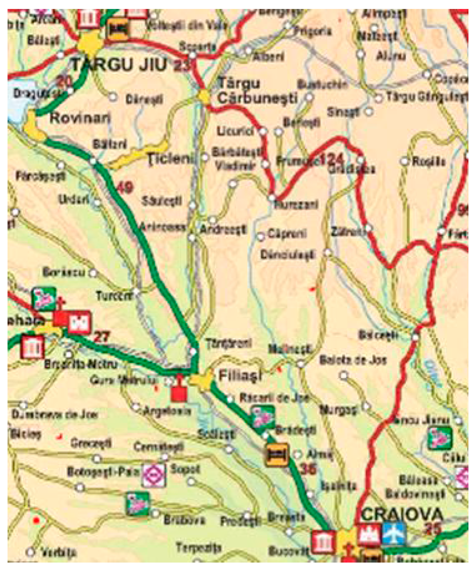
Note that the temperature decrease in the Jiu River water downstream of the wastewater outlets of the Rovinari, Turceni and Craiova power plants, respectively, is determined by the increase of Jiu River water flow due to its affluent rivers. These included the Jilt River (after the Rovinari power plant), the Gilort River and Motru River (after the Turceni power plant) and the Amaradia River (after the Craiova power plant), and can be seen in the map of the Jiu River in Figure 17.

Figure 17. Map of Jiu River.

Figure 17. Map of Jiu River.

4. Conclusions

The thermal pollution caused by three thermoelectric power plants located along a river has been successfully evaluated. Thermoelectric power plants are one of the main causes of thermal pollution. Such plants pump water directly from rivers, lakes or the ocean, to cool the turbine condensers. During the process, which usually involves once-through cooling, the water becomes warmer than the source water, so that the wastewater is returned to its source at temperatures significantly higher than the freshwater that originally entered the electric generation station. Discharging the warmer water to a river or lake can cause a significant environmental impact in terms of downstream thermal pollution, and wildlife can be affected.

In the present analysis, with three thermoelectric units of 330 MW operating in each of the Rovinari and Turceni power plants, and assuming an average river flow rate of 47 m³/s at the Rovinari site and 54.5 m³/s at the Turceni site, the effect of wastewater discharging in the Jiu River is found to be marginally acceptable.

Simultaneous operation of the thermoelectric units, in open circuit, (meaning, supplying fresh water from the river and discharging wastewater in the river, without using the cooling towers of the power plant) of the Rovinari, Turceni and Craiova power stations relies on the Jiu River flow, under the stability conditions for relevant environmental parameters. In an undeveloped regime of the river system, the flow of the Jiu River does not ensure the functioning in open circuit at the installed power of this chain of three coal-fired power plants connected in a cascade manner (from the cooling system viewpoint) along the Jiu River. If the coal-fired power plants of Rovinari and Turceni operate in open circuit (meaning without recirculation of the water in the cooling system of the power plant) at full capacity (with four and six thermoelectric units, respectively), then the environmental impact caused by wastewater thermal pollution, concerning aquatic ecosystems, can be significant. In these conditions, the operation of tower cooling systems in these power stations may prove necessary.

The EDF mathematic model of temperature evolution within the water of the Jiu River downstream from the outlet of the warm water pollutant vector allows an acceptable evaluation in terms of errors, for river lengths of 10–50 km.

For an acceptable evaluation, it is necessary to combine the simulation results (based on EDF mathematical pattern) with experimental tests for wastewater pollutant vector.

It would be useful to assess overall projections of the wastewater thermal pollutant vector, for both small and large distances.

Another environmental concern is related to abnormal weather conditions, such as arid summer or strong winter frost. Then, either the electrical capability of the coal-fired power plant (operating with a once-through cooling system) would decrease, or the aquatic ecosystems would be affected by the operation of the thermoelectric units. Then, from the viewpoint of environmental stewardship, a closed-cycle cooling system would be the Best Available Technology (BAT) for the thermoelectric power plants for reducing or avoiding adverse environmental impacts.

Within the framework of industrial ecology, as a sustainable policy of the thermoelectric power plants, it is also highlighted that the heat losses of the thermal wastewater of a power plant cooling system can be reduced by using the waste heat for heating local homes and/or greenhouses and/or industries.