3.1. Concept of a Collar Option Model for Hedging Change Order Risk
An option is a security that gives the owner the right to buy or sell an asset—subject to certain conditions—within a specified period of time [
20]. An option is a right, not an obligation, to take an action in the future. In financial markets, the most common types of options are call options and put options. A call option gives the owner the right to buy a stock at a predetermined exercise price on a specified maturity date. A put option can be viewed as the opposite of a call option: a put option gives its owner the right to sell the stock at a fixed exercise price [
21]. A collar option is more complex than a put option or a call option: it is a combination of a call option and a put option [
22]. A popular type of collar is the zero-cost collar. Typically, the proceeds from the sale of a call option are used to offset the cost of the put, eliminating the cost of the hedging instrument. The put insures the holder against any downward movement in the stock price below the strike price. Any movement above the strike price of the call is lost profit [
8].
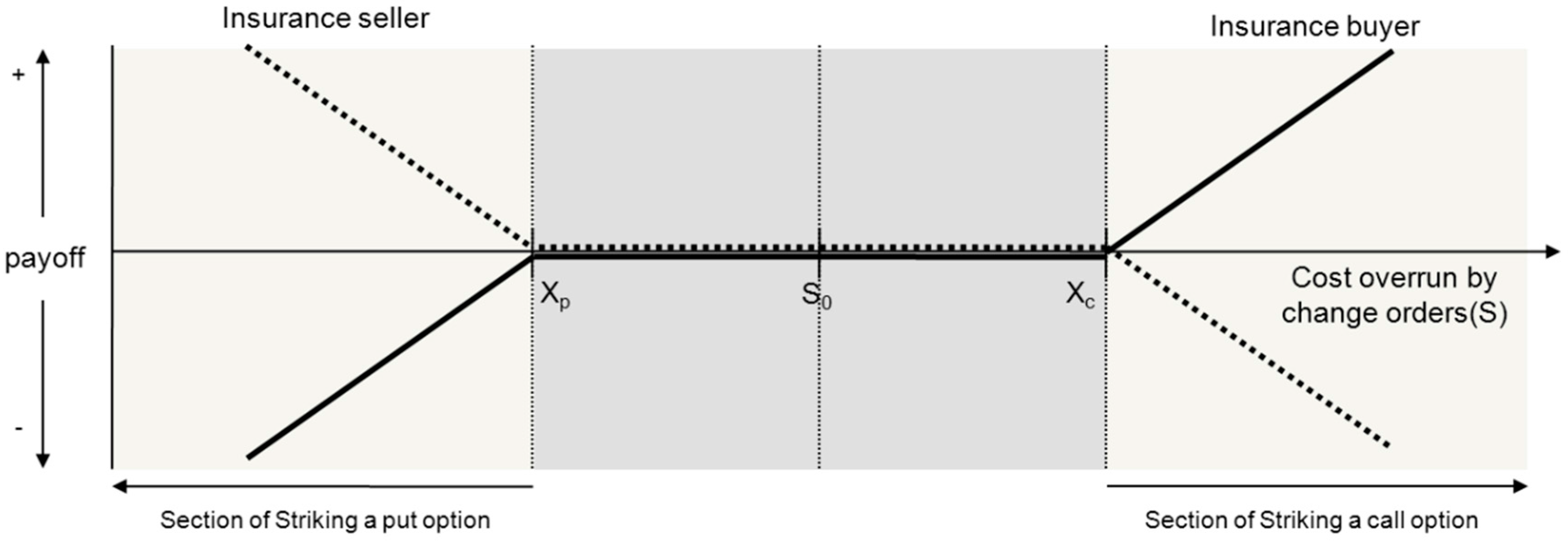
As shown in
Figure 1, the collar option model, which is a way of managing the cost overrun caused by change orders, consists of the insurance buyer’s section of striking a call option according to the increase in cost overrun and the insurance seller’s section of striking a put option according to the decrease in cost overrun. If
S0 is the current expected loss due to the cost overrun at present (
t = 0),
S0 is within the range of the strike price (
Xp) of the put option and the strike price (
Xc) of the call option.
Figure 1.
Concept of material contract model based on collar option.
Figure 1.
Concept of material contract model based on collar option.
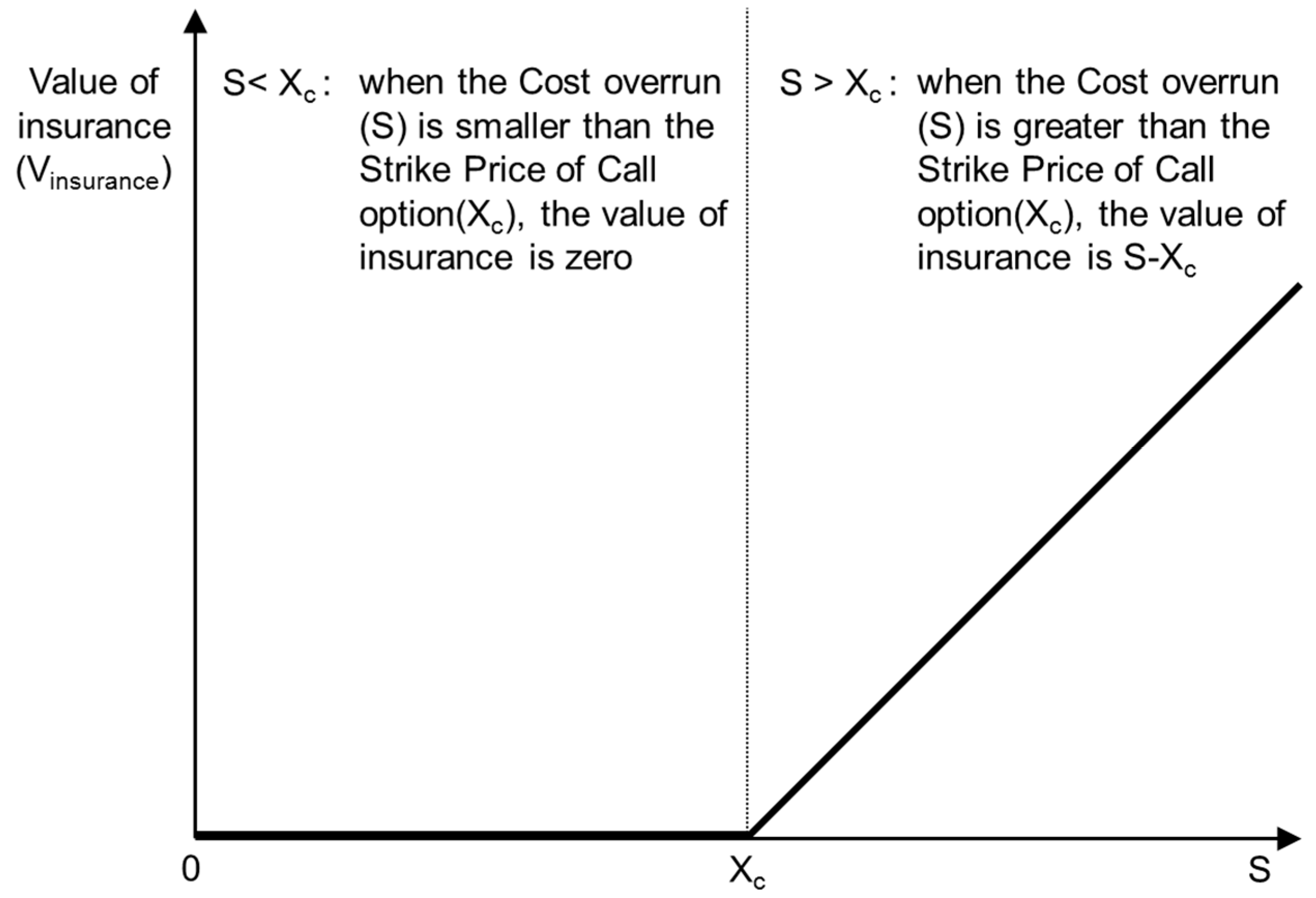
When the actual cost overrun caused by change orders exceeds the estimate, and
S exceeds
Xc, the insurance buyer exercises the call option, realizing the call option value shown in
Figure 2. Therefore,
Xc of the call option indicates the maximum permissible limit of the cost overrun caused by change orders in the corresponding project. In other words, the insurance becomes meaningless when the cost overrun is lower than
Xc;
i.e., the value of the insurance becomes zero. However, when the cost overrun exceeds
Xc, the insurance creates value because a hedge on the cost overrun can be placed through the insurance. In this case, the insurance seller’s side incurs a loss that is proportionate to the avoidance of the cost overrun caused by change orders placed through the insurance by the insurance buyer.
Figure 2.
Value of insurance depending on the increase in cost overrun.
Figure 2.
Value of insurance depending on the increase in cost overrun.
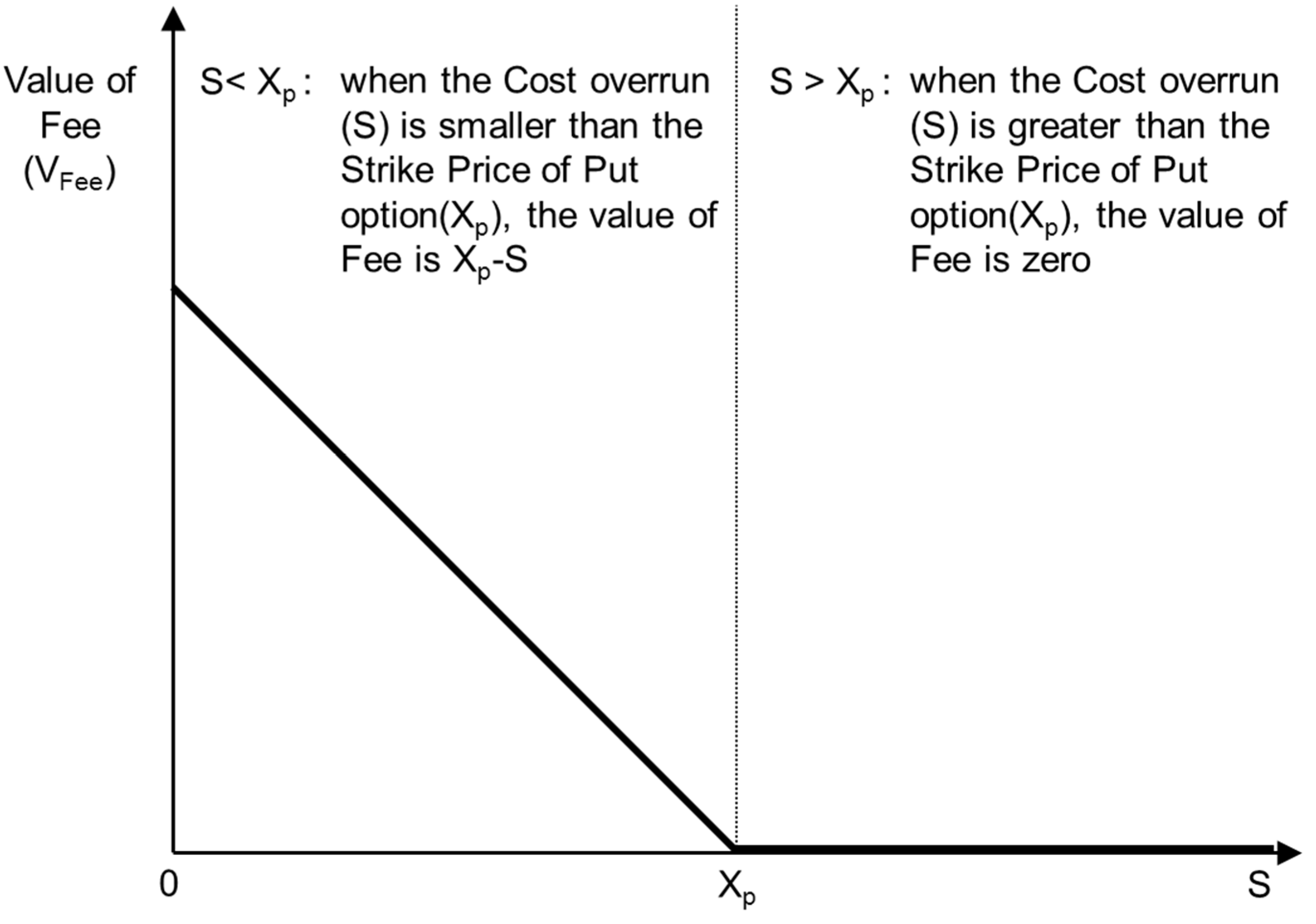
If the actual cost overrun caused by change orders is lower than expected, and
S is below
Xp, the insurance seller exercises the put option, realizing the put option value shown in
Figure 3. Therefore,
Xp of the put option indicates the starting point from which the insurance seller can secure a fee for providing insurance without baseline cost. In other words, when the cost overrun is lower than
Xp, the potential net profit margin of the insurance buyer is restored to the insurance seller.
Figure 3.
Value of fee depending on the decrease in cost overrun.
Figure 3.
Value of fee depending on the decrease in cost overrun.
In summary, the insurance premium is not fixed. When the cost overrun caused by change orders is lower than Xp, the insurance buyer pays the difference between the Xp value and the cost overrun as the insurance premium to the insurance seller. Therefore, the insurance premium varies according to changes in the cost overrun caused by change orders.
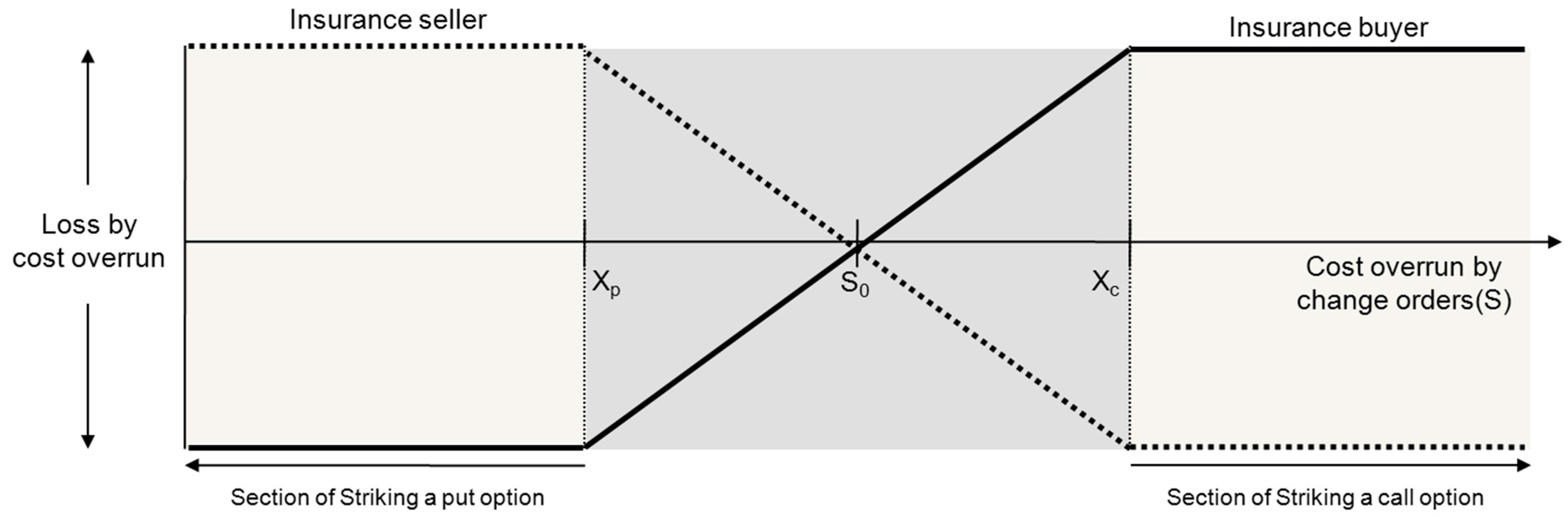
Ultimately, when the collar option model is applied, the loss that could occur because of the cost overrun caused by change orders can be controlled within a set range, as shown in
Figure 4.
Figure 4.
Range of loss caused by cost overrun when the collar option model is applied.
Figure 4.
Range of loss caused by cost overrun when the collar option model is applied.
To complete the collar option model, Xc and Xp must be selected so that the value of the call option and the put option are identical based on S0, the current expected loss because of cost overrun. In general, the expected loss of a construction project is estimated based on past data, using which a contingency is projected. That is, a contingency can be used to respond to a cost overrun that is lower than the expected loss. Thus, insurance has value when the cost overrun exceeds the expected loss. Therefore, in order to conduct an empirical analysis, this study estimates the expected loss caused by change orders. This study defines the expected loss as Xc. The value of the call and put options are identical. Therefore, the value of the insurance is calculated using Xc in order to produce Xp, the strike price of the put option.
3.2. Binomial Lattice Model for Calculating Option Value
Cox
et al. [
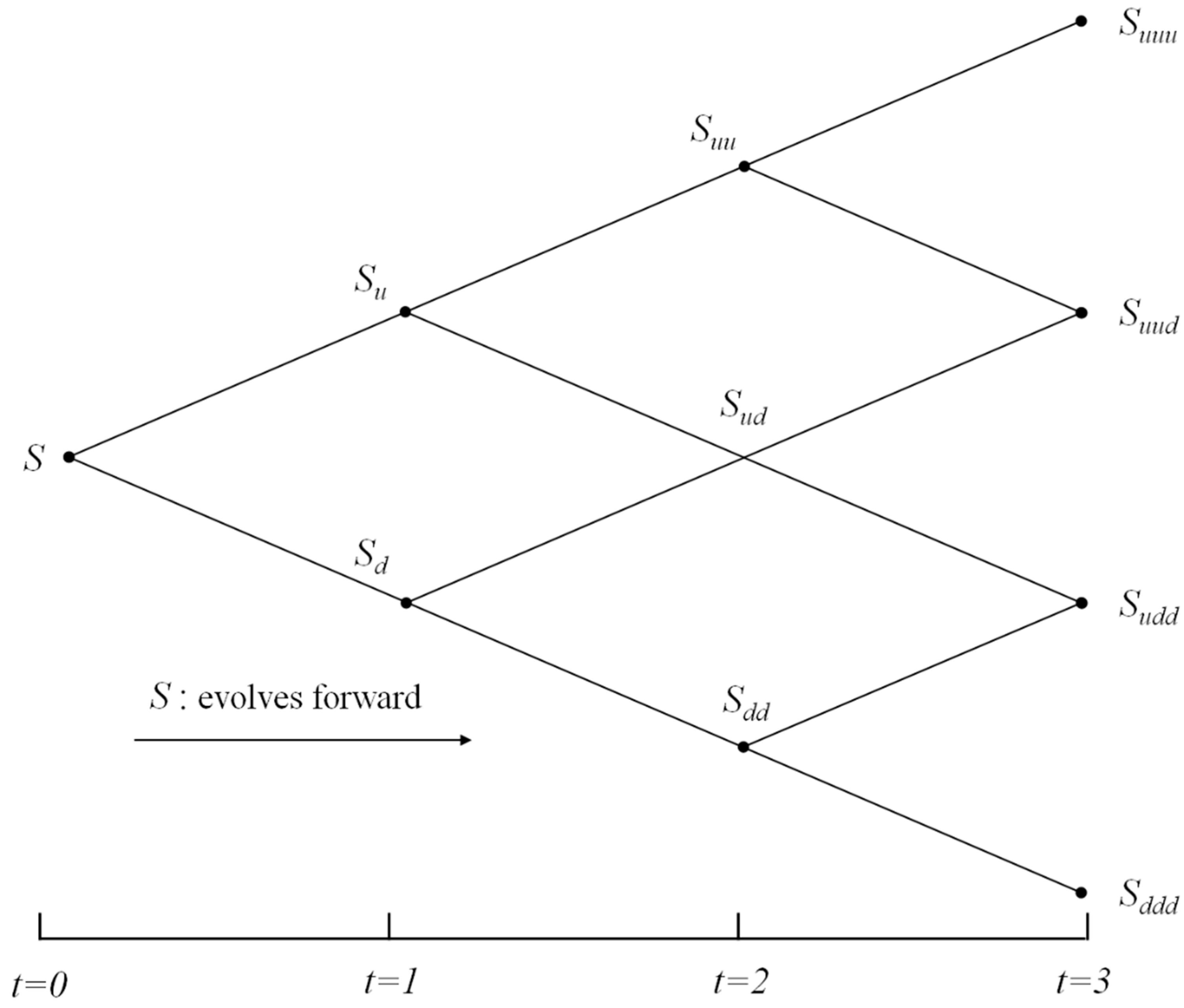
22] propose the binomial lattice model as a method for evaluating the option value under the assumption that the underlying asset fluctuates according to a binomial distribution. Binomial lattice models can solve complex and realistic option pricing problems. The binomial lattice model employs a two-stage calculation process. The first step is the creation of a binomial tree of distribution for the underlying asset, as shown in
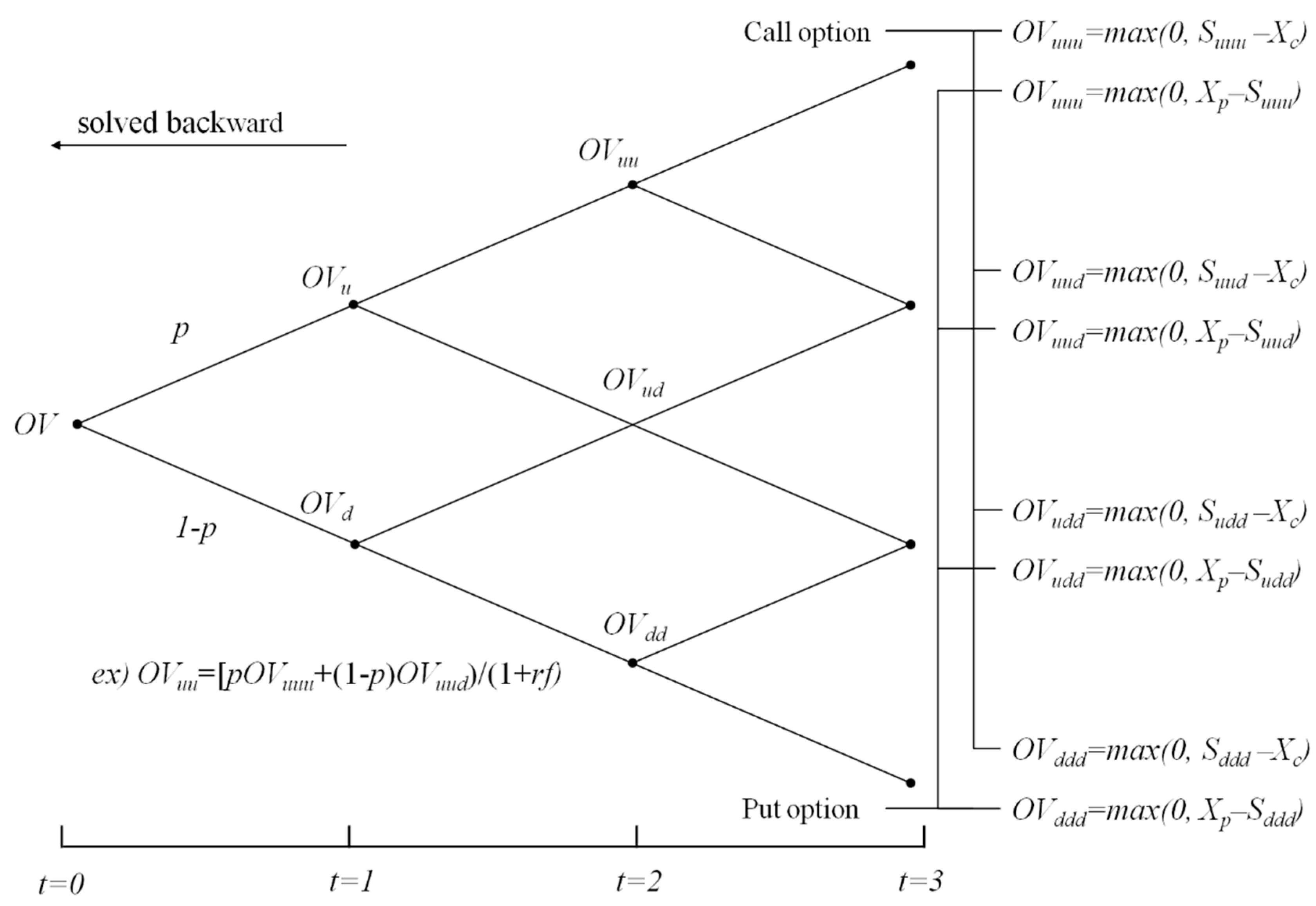
Figure 5. The second step is the creation of a binomial tree for calculating the option value, as shown in
Figure 6 [
23].
Figure 5.
Binomial tree of S’s distribution.
Figure 5.
Binomial tree of S’s distribution.
Figure 6.
Binomial tree for solving option value.
Figure 6.
Binomial tree for solving option value.
First, the underlying asset (
S) must be determined in the binomial tree. As shown in
Figure 1, this study assumes that the changes in option value are caused by the changes in cost overrun. Therefore, the current value of the cost overrun that is expected to occur because of change orders is modeled as the underlying asset (
S). As shown in
Figure 5, the binomial tree—with the underlying asset (
S) progressing through a forward process—models a case in which the cost overrun changes with time according to future uncertainty. The binomial tree in
Figure 5 operates by calculating the probability of increase (
u) and the probability of decrease (
d) repeatedly for the underlying asset (
S). The increase and decrease probabilities are calculated by default based on the volatility of the underlying asset. However, when the maximum and minimum values can be confirmed at the final point, the following equations can be used for the calculation [
24].
t = construction period (monthly)
= the maximum value of cost overrun that can occur during the construction period t
= the minimum value of cost overrun that can occur during the construction period t
The option value is calculated according to the backward process in
Figure 6, which is based on the binomial tree that is created through the forward process in
Figure 5. As shown in
Figure 6, the value of the call option or put option is calculated using the equation at the end of the binomial process. Equation (3) is an example of the correlation between the node at t–1 and the two nodes at t. In other words, Equation (3) indicates that the OV
uu node is obtained by calculating the expected value using the OV
uuu node, OV
uud node, and risk-neutral probabilities (
p) and discounting it using the risk-free rate.
Finally, the option value (OV node) at
t = 0 can be calculated by applying this equation to other nodes. The risk-neutral probabilities (
p) are calculated according to Equation (4). In this paper,
rfmonth is the monthly risk-free rate for which the three-year government bond interest rate is utilized.
This study uses the binomial lattice model to produce the call option value and calculate the initial insurance value. Subsequently, this model is used to produce the strike price of an identically-valued put option in order to derive the point at which profit is generated for the insurance seller.


