2. A Brief Survey of the Empirics of Regional Income Convergence
The literature on regional income convergence presents a variety of empirical approaches. Following the seminal contribution by Baumol [
11] later refined by Barro and Sala-i-Martin [
3], a large number of empirical studies has made use of growth regressions to see whether poor regions tend to grow faster than rich ones, thereby implying regional income convergence [
12,
13,
14,
15,
16,
17]. Among others, Carlino and Mills [
12] provide evidence for per capita income convergence for US regions over the period from 1929 to 1990 after allowing for a structural break in 1946. Tsionas [
17] employs both β- and σ-convergence tests, thereby concluding against the convergence of per capita incomes over the period 1977 to 1996. Choi [
14] applies multiple panel data techniques to state per capita output over the period from 1929 to 2001 and finds that convergence has proceeded among geographically neighboring states rather than among distant states. More recently, Mello [
16] finds that relative income shocks for the US states are persistent but eventually die out, supporting the stochastic convergence hypothesis.
The results of Rey and Montouri [
18] represent the first detailed evidence on the role of spatial effects in a regional income convergence study. Although their study reconsiders the question of income convergence from a spatial econometric perspective, it should be noted that they use states as their observational units in the analysis of regional convergence. States might be the most relevant units of policy-making; however, the high degree of spatial aggregation might mask the existence of different growth trajectories below the state level. With respect to growth empirics, the treatment of space in the analysis of regional economic convergence has only recently begun to attract attention. Ertur
et al. [
19], Dall’erba
et al. [
20], and Ramajo
et al. [
6] investigated the role of spatial effects in the analysis of economic convergence processes among NUTS (Nomenclature of Units for Territorial Statistics) level-2 regions in the EU countries. More recently, several empirical studies find increasing polarization in per capita income across regions and explain this effect as primarily the result of the formation of geographical clusters across regions within countries [
21,
22,
23,
24,
25]. In light of these findings, a clear need exists to develop a spatially explicit analytical model for the analysis of regional economic convergence.
Most of the empirical work on regional income convergence has been carried out using cross-sectional regressions that relate the initial per capita income level for a group of regional economies to their subsequent per capita income growth rates. Although earlier studies were based on cross-sectional estimations, resorting to panel estimations enables us to take potential omitted variable bias into account [
26,
27,
28]. The panel data approach makes it possible to account for unobservable cross-section specific characteristics such as the initial level of technology, taking potential omitted variable bias problem into account by allowing for technological differences across regions in the form of individual effects [
4,
9,
10]. Atems [
26] examines the dynamic relationship between income inequality and economic growth using US county-level data and finds a significant negative relationship between inequality and growth across the 3109 counties of the US. Recently, the growth regression has been extended to consider the role of spatial effects in the panel data analysis [
27,
29]. Using the dynamic spatial dependence model for panel data, Atems [
27] examines the spatial dynamics of income inequality and economic growth for the 3109 counties of the US over the period from 1970 to 2007. Consequently, there is need to specify a panel data model that adequately captures the spatial dynamics of regional income convergence.
It should be noted that the issue of which spatial units are most appropriate for the analysis of regional income convergence within a country has received little attention despite the fact that geography has played an important role in the regional income convergence process [
30]. Due primarily to data availability, administratively defined regions, such as US states and NUTS level-2 regions in the EU countries, are commonly used in the empirical analysis of regional income convergence [
8,
18,
19,
31,
32]. Whether these spatial units of analysis are suitable for analyzing regional income convergence is questionable because they are neither economically homogeneous entities nor self-contained with respect to labor markets [
30,
33,
34,
35]. Indeed, spatial processes occur within the boundaries of geographic areas characterized by functional linkages and dependencies [
33,
36,
37].
From a spatial econometric point of view, the use of administratively defined regions as spatial units of analysis may induce nuisance spatial dependence, which may result from a mismatch between the geographic boundaries of the economic processes and the boundaries of the observational units [
38]. As noted by Magrini [
30], the use of functionally defined regions could be useful as a strategy for minimizing nuisance spatial dependence. From a theoretical perspective that spatial processes occur within the boundaries of geographic areas characterized by functional linkages and dependencies, spatial units that are not only more disaggregated than states but also functional rather than administrative are likely to be more accurate than those used in inter-state convergence studies [
39]. As clearly shown by Martin [
35], more appropriate spatial units of analysis would be the economic areas in the contiguous US states, as defined by the Bureau of Economic Analysis (BEA). As far as we are aware, however, few empirical studies have been conducted using these spatial units that are functionally meaningful in terms of the economic processes with which to generate regional income convergence.
In light of these considerations, this article aims to investigate the process of regional income convergence process over the period 1969 to 2009 using data for 177 economic areas in the conterminous US states, as defined by BEA as of November 2004. BEA’s economic area is defined as a functional area which comprises one or more economic nodes—metropolitan or micropolitan statistical areas that serve as regional centers of economic activity—and the surrounding counties that are economically related to the nodes [
40]. These economic areas represent the relevant regional markets for labor, products and information. The main factor used in determining the economic relationships among counties is labor commuting patterns that delineate local labor markets, so each economic area includes, as far as possible, the place of work and the place of residence of its labor force. Data on per capita income for economic areas are drawn from the Regional Economic Information System (REIS) of BEA. All of the per capita income data are expressed in 2005 chain-weighted dollars.
3. Exploratory Spatial Data Analysis
In the first step of our analysis, we examine the potential presence of spatial dependence in per capita income for 177 economic areas by using exploratory spatial data analysis (ESDA) techniques. Spatial dependence, often also referred to as spatial autocorrelation, can be considered to be the existence of a functional relationship between what happens in a region and what happens in its neighboring regions [
38]. Positive spatial autocorrelation occurs when similar values for a variable are spatially clustered together, whereas negative spatial autocorrelation appears when dissimilar values are clustered in space.
By using Moran’s
I statistics, we test for global spatial autocorrelation in initial per capita income. The
I statistic is expressed as follows:
where
n is the number of economic areas,
wij is the element in a spatial weights matrix
W = [
wij], designating economic areas as neighbors when they share a common border (
i.e., the elements
wij is 1 if economic areas
i and
j share a common border and 0 otherwise),
xi is the natural logarithm of per capita income in the economic area
i (measured as a deviation from the mean value), and
s0 is a normalizing factor equal to the sum of the elements of the weights matrix,
i.e.,
[
38]. The value of the
I statistic ranges from −1 for negative spatial autocorrelation to 1 for positive spatial autocorrelation. Over the entire economic areas, if similar values are more likely than dissimilar values between neighbors, the
I statistic tends to be positive, and
vice versa.
The statistical significance of the
I statistic is calculated by applying a randomization, given non-normality for distributions of per capita income.
Table 1 presents the results of Moran’s
I test on regional per capita income, which is performed for each of the eight cross-sections with 177 economic areas, which comprise the full panel of data. The
I statistic for the 1969 per capita income is 0.541, indicating that the distribution of initial per capita income is spatially clustered as the statistic is significant with
p < 0.001. Although the magnitude of the spatial autocorrelation seems to weaken over the period, the spatial autocorrelation is still highly significant in every year. This result reveals that there is very strong evidence of positive spatial dependence in the distribution of the initial regional per capita income. A similar result is found for the growth rate of per capita income from 1969 to 2009, yielding the
I statistic of 0.610 with
p < 0.001. These results suggest that the regional income observations are spatially related and therefore should not be assumed to be independent observations.
Table 1.
Spatial autocorrelation of per capita income and income growth, 1969–2009.
Table 1.
Spatial autocorrelation of per capita income and income growth, 1969–2009.
| Variable | Moran’s I | Variable | Moran’s I |
|---|
| ln (y69) | 0.5415 | ln (y74/y69) | 0.4452 |
| ln (y74) | 0.5165 | ln (y79/y74) | 0.3543 |
| ln (y79) | 0.4402 | ln (y84/y79) | 0.4926 |
| ln (y84) | 0.3478 | ln (y89/y84) | 0.7166 |
| ln (y89) | 0.3925 | ln (y94/y89) | 0.5470 |
| ln (y94) | 0.2679 | ln (y99/y94) | 0.1263 |
| ln (y99) | 0.2381 | ln (y04/y99) | 0.3825 |
| ln (y04) | 0.2428 | ln (y09/y04) | 0.4973 |
| ln (y09) | 0.2511 | ln (y09/y69) | 0.6104 |
From a more disaggregated view of the nature of spatial autocorrelation, the Moran scatterplot is employed to capture the local structure of spatial association. The Moran scatterplot decomposes global spatial association into the four different quadrants, which correspond to the four types of local spatial association between an economic area and its neighbors: (i) HH: high-high association (a high per capita income area surrounded by high per capita income neighbors); (ii) LL: low-low association (a low per capita income area surrounded by low per capita income neighbors); (iii) HL: high-low association (a high per capita income area surrounded by low per capita income neighbors); (iv) LH: low-high association (a low per capita income area surrounded by high per capita income neighbors). Quadrants HH and LL represent positive spatial association indicating spatial clustering of similar values while quadrants HL and LH refer to negative spatial association.
As shown in
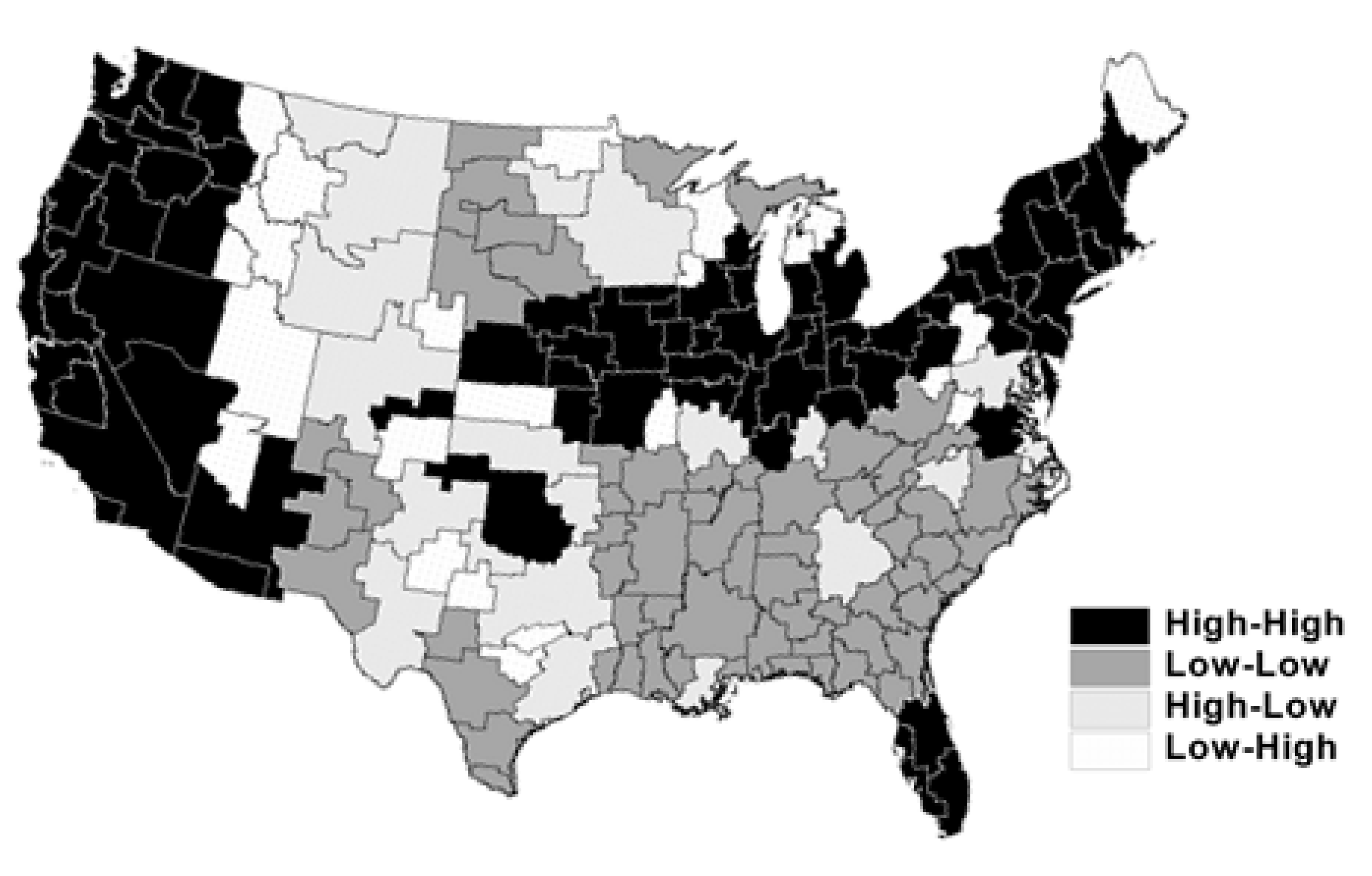
Figure 1, the Moran scatterplot reveals the predominance of HH and LL clustering types of per capita income in the initial year, 1969. Approximately 76% of economic areas fall in either HH or LL quadrants of the scatterplot. In conjunction with the Moran scatterplot, the Moran scatterplot map provides a visual impression on the presence of spatial heterogeneity in the form of spatial clusters of rich and poor regions. For the per capita income levels in 1969, the economic areas in the northeastern and western regions tend to cluster in HH form, while those in the southern regions tend to cluster in LL form (
Figure 2). These results suggest that the convergence process, if it exists, could be different between the two regions constituted by HH and LL clustering spatial regimes.
Figure 1.
Moran scatterplot for log per capita income, 1969.
Figure 1.
Moran scatterplot for log per capita income, 1969.
Figure 2.
Moran scatterplot map for log per capita income, 1969.
Figure 2.
Moran scatterplot map for log per capita income, 1969.
4. Spatial Dependence in the Panel Data Convergence Model
One of the major advantages of the panel data approach to convergence is that it can correct the omitted variable bias problem of the cross-section convergence regression by allowing for technological differences across economic areas in the form of individual effects [
28]. The traditional β-convergence model can be reformulated in the panel data context as follows:
where
i is an index for the cross-sectional dimension (spatial units), with
i = 1,…,
n, and
t is an index for the time dimension (time periods), with
t = 1,…,
T. Using customary notation,
yi,t represents the per capita income at time
t for economic area
i, α
i is the constant term parameter, μ
i is the spatial specific fixed effect, φ
t is the time-period specific effect, and
uit is an independent and identically distributed error term for
i and
t with zero mean and constant variance. The parameter β is of particular interest, because it can be seen as a test of the catching up. A negative estimate for β supports the convergence hypothesis since such an estimate would suggest that the growth rates in per capita income over the period are negatively related with initial per capita income levels. Spatial specific effects control for all time-invariant technological differences across economic areas whose omission could bias the estimates in a typical cross-sectional study, while time-period specific effects control for all spatial-invariant variables whose omission could bias the estimates in a typical time-series study [
41]. In general, the spatial fixed effects model is favored when the regression analysis is applied to a precise set of regions; by contrast, the random effects model is an appropriate specification if a certain number of individuals are randomly drawn from a large population of reference [
41]. Because our data set consists of the observations of the same 177 economic areas (
n = 177), we estimate the fixed effects panel data model.
As is commonly recognized, regional income growth and convergence are fundamentally long-run phenomena. The switch from a single cross-section to a panel framework is made possible by dividing the entire period into several shorter time spans. This is the most common approach to using five-year time intervals rather than a year-by-year specification, because short-run variations in income growth rates are inevitably influenced by business cycle fluctuations [
9,
28,
29,
42]. In line with these motivations, we use five-year growth rates rather than a year-by-year specification. Considering the entire period from 1969 to 2009, we have eight five-year time spans (
T = 8) for each economic area: 1969–1974, 1974–1979, 1979–1984, 1984–1989, 1989–1994, 1994–1999, 1999–2004, and 2004–2009. Thus, the number of observations used in the model estimation is:
nT = 177 × 8 = 1416.
The concept of traditional β-convergence treats regions as “isolated islands”. It does not capture the fact that one region’s economic destiny is dependent on those of other regions. Indeed, the evolution of each region is closely related to the evolution of, at least, neighboring regions. From a theoretical point of view, the inclusion of spatial dependence in regional income convergence models has been motivated by Armstrong [
43], Rey and Montouri [
18], and López-Bazo
et al. [
44]. In this context of spatial dependence, the distribution of regional per capita income is unlikely to be spatially independent and random. The traditional fixed effects convergence model can be reformulated in the spatial dependence context as follows:
where ρ is the spatial autoregressive coefficient and
wij is an element of an
n ×
n spatial weights matrix
Wn such that
wij = 1 if economic areas
i and
j share a common border and zero otherwise. The spatial weights matrix is row-standardized such that the elements in each row sum to one. For a particular economic area, the resulting spatial lagged dependent variable can be considered to be a spatially weighted average of all other neighboring economic areas’ per capita income growth. For this fixed effects spatial lag model, the spatial autoregressive coefficient captures the spatial interaction effect, indicating the extent to which the growth rate of per capita income in a particular economic area is affected by the growth rate of its neighboring economic areas.
As explained in detail by Abreu
et al. [
33] and Arbia
et al. [
9], the estimated coefficient of initial per capita income in the spatial lag model includes only the direct marginal effect of an increase in the initial per capita income, excluding all indirect and induced effects, while in the standard model of Equation (2) this coefficient represents the total marginal effect of an increase in the initial per capita income. In stacked matrix form, Equation (3) can be written as:
where
g is an
nT × 1 vector of per capita income growth over each time period,
y is an
nT × 1 vector of log per capita income levels in the initial year over each time period,
ι is an
nT × 1 vector of ones associated with the constant term parameter α, β is the unknown parameter in the analysis of convergence, ρ is the spatial autoregressive parameter, μ is an
nT × 1 vector of spatial specific fixed effects, φ is an
nT × 1 vector of time-period specific fixed effects, and
u is an
nT × 1 vector of independent and identically distributed error terms for
i and
t with zero mean and constant variance.
The spatial weights matrix WnT for the panel dimension is a non-negative nT × nT block-diagonal matrix of known constants describing the arrangement of the spatial units in the sample. More specifically, we can express this WnT matrix as the Kronecker product of a T × T identity matrix and an n × n spatial weights matrix IT ⊗ Wn, where the elements of wij of Wn reflect the relative degree of the connection of spatial unit j to i. The elements of the block-diagonal submatrices of WnT specify the spatial dependence structure among the economic areas. Each block represents a group of spatial units that interact with each other but not with observations in other groups. Because of the block structure, economic areas interact with each other within the same period, but not with economic areas in other periods. We assume that the block-diagonal submatrix Wn is constant over time and that the panel is balanced. The diagonal elements of the block-diagonal submatrices of WnT are assumed to be zero, since no spatial unit can be its own neighbor. Each block-diagonal submatrix is also row-standardized to have row-sums of unity such that the resulting nT × 1 vector of the spatial lagged dependent variable WnTg will be equal to the spatially weighted average of the growth rates of per capita income of all other neighboring economic areas.
Equation (4) can be rewritten in reduced form as follows:
where
represents the spatial multiplier matrix. The spatial multiplier effect can be decomposed as follows:
The first term on the right-hand side is the direct effects on the diagonal, which represents the effects on the per capita income growth of a marginal change in the initial per capita income of economic area
i. The second term is the indirect effects in the off-diagonal for the neighbors of economic area
i, which represents spillovers of the direct effects of the first-order neighbors of economic area
i. The third and higher-order terms capture spatial spillovers induced by the direct and indirect changes in the first and second terms. As a consequence, the indirect effects are spillovers of the direct effects of the first-order neighboring economic areas, while the induced effects are spatial spillovers induced by the direct and indirect effects of the higher-order neighboring economic areas [
9,
33,
45,
46].
An alternative way to incorporate spatial dependence effects is to reformulate the traditional fixed effects convergence specification into the following model:
with
where λ is the spatial autocorrelation coefficient and ε
it is assumed to be normally distributed independent of the explanatory variable with zero mean and constant variance. This specification is called the fixed effects spatial error model, which is relevant when the spatial dependence works through the error process in that the errors from different economic areas may display spatial autocorrelation. Spatial error dependence may be interpreted as a “nuisance” in that it reflects spatial autocorrelation in measurement errors or in variables that are otherwise not crucial to the model. For this fixed effects spatial error model, a random shock in a particular economic area will not only affect the growth rate in that economic area but will also impact the growth rates of other economic areas. The estimated coefficient of initial per capita income in the spatial error model includes its total marginal effect, while in the spatial lag model, it captures only the direct marginal effect of an increase in the initial per capita income excluding indirect and induced effects [
9,
33,
45,
46].
A limitation of spatial lag and error models is that the dependent variable is influenced by independent variables in neighboring locations as well. If the non-spatial model is rejected (on the basis of the Lagrange multiplier (LM) tests) in favor of the spatial lag model or the spatial error model, we should consider the spatial Durbin model, which include both endogenous and exogenous spatial interaction effects. This model extends the spatial lag model with spatially lagged explanatory variables. The spatial Durbin model can be written as follows:
where γ is the spatial cross-regressive parameter. This model could be estimated with or without the implied parameter restrictions [
46,
47]. Model specification tests are usually conducted to determine which mode is appropriate for the empirical study.
In the first column of
Table 2, the ordinary least squares (OLS) estimates of the traditional non-spatial model are presented. As evidenced in a large number of Monte Carlo simulation experiments [
48], the joint use of the LM tests for spatial lag dependence and spatial error dependence provides the best guidance for model specification. If the LM-lag is significant while the LM-error is not, then it is likely that a spatial lag dependence model is the correct specification. If on the other hand the LM-error model is significant while the LM-lag is not, then the spatial error dependence model is the correct specification. However, when both LM test statistics have high values indicating significant spatial dependence, the one with the higher robust LM test statistic tends to indicate the correct specification. In this model, the robust LM tests for spatial dependence show that there is an indication of misspecification in the form of spatial error dependence.
According to the LM test results for spatial dependence in the model, the OLS estimates suffer from a misspecification due to omitted spatial dependence. The spatial econometric literature has shown that OLS estimation is inappropriate for models incorporating spatial effects [
38,
46]; therefore, we estimate the spatial dependence models by the method of maximum likelihood (ML) [
38,
49]. The results of the ML estimation of the spatial dependence models are shown in columns 2–4 of
Table 2. As shown in columns 2 and 3 of
Table 2, explicitly taking the spatial dependence into account results in a slower estimated annual rate of convergence than that based on the OLS estimate. The implied convergence rate
θ is calculated using
, where
t is the number of years in the period. Using data on per capita incomes in the 48 contiguous US states over the period 1929 to 2011, Breuer
et al. [
31] find an implied convergence rate of 1.75% per year based on the estimates from the traditional cross-sectional model for the 48 US states.
Table 2 indicates that the implied annual rate of convergence over the period associated with the spatial cross-sectional model ranges from 0.08% to 0.16%, which is much lower than the values typically found for the 48 contiguous US states.
Table 2.
Estimation results for the spatial dependence models without fixed effects.
Table 2.
Estimation results for the spatial dependence models without fixed effects.
| Variable | (1) Non-Spatial Model | (2) Spatial Lag Model | (3) Spatial Error Model | (4) Spatial Durbin Model |
|---|
| Constant | 0.998 (0.000) | 0.331 (0.000) | 0.707 (0.000) | 0.281 (0.000) |
| Init. per capita inc. (β) | −0.090 (0.000) | −0.031 (0.000) | −0.061 (0.000) | −0.050 (0.000) |
| Spatial lag (ρ) | | 0.741 (0.000) | | 0.749 (0.000) |
| Spatial error (λ) | | | 0.746 (0.000) | |
| Spatial cross-regr. (γ) | | | | 0.024 (0.008) |
| Convergence rate (%) | 0.236 | 0.079 | 0.157 | 0.128 |
| LM-lag | 1075.010 (0.000) | | | |
| Robust LM-lag | 7.800 (0.005) | | | |
| LM-error | 1123.062 (0.000) | | | |
| Robust LM-error | 55.852 (0.000) | | | |
| R-sq | 0.178 | | | 0.584 |
| Corr-sq | | 0.173 | 0.178 | 0.178 |
| LIK | 2097.700 | 2478.943 | 2477.868 | 2482.350 |
| Observations | 1416 | 1416 | 1416 | 1416 |
The econometrics of panel data models with spatial effects is an active area of research, as evidenced by the growing number of papers on the topic [
46,
50]. However, none of the standard econometric packages include built-in facilities to carry out spatial panel econometrics. In this regard, Elhorst [
51] provides Matlab routines on his website (
http://www.regroningen.nl/elhorst) for the fixed effects and random effects spatial lag model, as well as the fixed effects and random effects spatial error model. We take the Matlab routines to estimate spatial panel data models. Of these models, the spatial lag model, the spatial error model, and the spatial Durbin model are extended to include spatial and time-period fixed effects.
Table 3 presents the estimated results for the fixed effects spatial panel data models to take potential omitted variable bias into account. The estimation of spatial panel data models has been extensively discussed in Elhorst [
47,
50] and Lee and Yu [
52]. Elhorst [
47,
50] reviews the issues that arise in the estimation of spatial panel data models and presents the ML estimators of the spatial panel data models. Of these, the spatial lag model, the spatial error model, and the spatial Durbin model are extended to include spatial and time-period fixed effects. The results of the ML estimation of the spatial panel data models are shown in columns 2–4 of
Table 3. Column 1 of
Table 3 reports the estimation results of the spatial and time-period fixed effect non-spatial model of Equation (2), and the test results to determine whether the spatial lag model or the spatial error model is more appropriate. The fixed-effects convergence model is conditional in that it considers the potential omitted variable bias problem. It does this by allowing for all time-invariant technological differences across economic areas and all spatial-invariant variables in the process of regional income convergence. The value of the estimated coefficient of initial per capita income shows the presence of convergence over the period.
Table 3.
Estimation results for the spatial panel data models with fixed effects.
Table 3.
Estimation results for the spatial panel data models with fixed effects.
| Variable | (1) Spatial and Time-Period Fixed Effects Non-Spatial Model | (2) Spatial and Time-Period Fixed Effects Spatial Lag Model | (3) Spatial and Time-Period Fixed Effects Spatial Error Model | (4) Spatial and Time-Period Fixed Effects Spatial Durbin Model |
|---|
| Init. per capita inc. (β) | −0.475 (0.000) | −0.340 (0.000) | −0.506 (0.000) | −0.511 (0.000) |
| Spatial lag (ρ) | | 0.633 (0.000) | | 0.689 (0.000) |
| Spatial error (λ) | | | 0.711 (0.000) | |
| Spatial cross-regr. (γ) | | | | 0.373 (0.000) |
| Convergence rate (%) | 1.611 | 1.039 | 1.763 | 1.788 |
| LM-lag | 623.252 (0.000) | | | |
| Robust LM-lag | 2.949 (0.000) | | | |
| LM-error | 812.811 (0.000) | | | |
| Robust LM-error | 192.507 (0.000) | | | |
| R-sq | 0.236 | | | |
| Corr-sq | | 0.185 | 0.236 | 0.238 |
| LIK | 2448.300 | 2679.239 | 2731.071 | 2731.318 |
| Wald test-spatial lag | | | | 98.360 (0.000) |
| LR test-spatial lag | | | | 104.159 (0.000) |
| Wald test-spatial error | | | | 0.565 (0.452) |
| LR test-spatial error | | | | 0.495 (0.482) |
| Observations | 1416 | 1416 | 1416 | 1416 |
For the base model in column 1 of
Table 3, specification tests for spatial dependence are carried out using the LM tests for spatial error dependence and spatial lag dependence. According to the decision rule evidenced in a large number of Monte Carlo simulation experiments [
48], the robust LM tests for spatial dependence show that there is a strong indication of misspecification in the form of spatial error dependence in the spatial and time-period fixed effects non-spatial model. This suggests that the spatial and time-period fixed effects spatial error model should be considered for the appropriate specification. To investigate whether or not the fixed effects are jointly significant, we performed a likelihood ratio (LR) test, which is based on the log-likelihood function value of the model. The null hypothesis that the spatial fixed effects are jointly insignificant is rejected (400.518, with 177 degrees of freedom,
p < 0.01). Similarly, the null hypothesis that the time-period fixed effects are jointly insignificant is rejected (583.668, with eight degrees of freedom,
p < 0.01). These results imply that the spatial and time-period fixed effects model should be considered for the appropriate specification.
The estimated results for the spatial and time-period fixed effects models with spatial effects are presented in columns 2 and 3 of
Table 3. We find that the estimated coefficient of the initial per capita income is negative and statistically significant, confirming the hypothesis of regional income convergence over the period under consideration. Compared to the estimation result of the fixed effects non-spatial model, the absolute value of the estimated coefficient of the initial per capita income decreases in the fixed effects spatial lag model and increases in the fixed effects spatial error model. We now consider the spatial and time-period fixed effects spatial Durbin model of regional income convergence. Its results are reported in column 4 of
Table 3. Compared to the estimation results of the fixed effects spatial lag and error models, the absolute value of the estimated coefficient of the initial per capita income is higher in the fixed effects spatial Durbin model. We find that the estimated coefficient of the initial per capita income is negative and statistically significant, confirming the hypothesis of regional income convergence over the period under consideration. The associated annual convergence rate over the period is 1.79%. The inclusion of both endogenous and exogenous spatial interaction effects leads to an increase in the magnitude of the absolute value of the estimated coefficient of the initial per capita income.
The spatial Durbin model can be used to test the hypotheses
H0: γ = 0 and
H0: γ + ρβ = 0. To test the null hypothesis that the fixed effects spatial Durbin model can be simplified to the spatial error model,
i.e.,
H0: γ + ρβ = 0, we performed a Wald or likelihood ratio (LR) test. The test results imply that the fixed effects spatial Durbin model can be simplified to the fixed effects spatial error model, while the null hypothesis for the fixed effects spatial lag model
H0: γ = 0 is rejected in favor of the fixed effects spatial Durbin model. These results imply that the fixed effects spatial error model best describes the data, if the robust LM tests also pointed to the spatial error model. As shown in column 3 of
Table 3, the estimated coefficient of the initial per capita income is negative and statistically significant, confirming the hypothesis of regional income convergence over the period. The associated annual convergence rate over the period is 1.76%. The inclusion of the spatial error autocorrelation leads to an increase in the magnitude of the absolute value of the estimated coefficient of the initial per capita income. This finding confirms that economic areas are open to a range of socioeconomic flows and exhibit spatial proximity in convergence.
The convergence speed is lower in the fixed effects spatial lag model than it is in the fixed effects spatial error model, as is the case in the results of Abreu
et al. [
33] and Arbia
et al. [
9], This is because the estimated coefficient of initial per capita income in the spatial lag model captures only the direct marginal effect of an increase in the initial per capita income, while in the spatial error model it represents its total marginal effect including all indirect and induced effects. This result implies that the growth rate in a specific economic area will be not only directly affected by an exogenous shock introduced into that economic area but, through the spatial multiplier effect, also more impacted by both indirect effects of the first-order neighboring economic areas and induced effects of the higher-order neighboring economic areas [
9,
33].


