Parametric Assessment of Water Use Vulnerability Variations Using SWAT and Fuzzy TOPSIS Coupled with Entropy

Abstract

This study assessed the water use vulnerability to include the uncertainty of the weighting values of evaluation criteria and the annual variations of performance values using fuzzy TOPSIS coupled with the Shannon entropy method. This procedure was applied to 12 major basins covering about 88% territory of South Korea. Hydrological components were simulated using Soil and Water Assessment Tool (SWAT) of which parameters were optimally calibrated using SWAT-CUP model. The 15 indicators including hydrological and anthropogenic factors were selected, based on three aspects of climate exposure, sensitivity and adaptive capacity. Their weighting values were objectively quantified using the Entropy method. All performance values of 12 basins obtained from statistic Korea and SWAT simulation were normalized with the consideration of the annual variations from 1991 to 2014 using triangular fuzzy numbers (TFNs). Then, Fuzzy Technique for Order of Preference by Similarity to Ideal Solution (TOPSIS) technique was used to quantify the water use vulnerability and rank 12 basins as follows: A12 (Hyeongsan River) > A6 (Seomjin River) > A5 (Youngsan River) > A8 (Mangyung River) > A2 (Ansung River) > A9 (Dongjin River) > A10 (Nakdong River) > A3 (Geum River) > A4 (Sapgyo River) > A11 (Taehwa River) > A7 (Tamjin River) > A1 (Han River). This framework can be used to determine the spatial priority for sustainable water resources plan and applied to derive the climate change vulnerability on sustainable water resources.

1. Introduction

Ensuring sufficient water supply is essential for the survival and sustenance of human and ecosystems [1]. However, the recent climate variation has severely affected the hydrological cycle. The IPCC report concluded that it is highly likely that “the negative impacts of climate change on freshwater systems outweigh its benefits” with runoff declining in most streams and river [2]. Therefore, insufficient water availability for essential ecosystem functions and services can lead to ecosystem degradation with consequent impacts on overall water scarcity and human well-being [3].

Many hydrological models had been used to quantify the water scarcity amount for a long time. Recently, the rainfall runoff models coupled with GIS program were often developed and applied to sustainable water resources vulnerability. Among them, the SWAT (Soil and Water Assessment Tool) [4] has been frequently used to simulate the spatially coarse daily runoff by combining the high resolution Digital Elevation Model (DEM) with landuse and soil maps. SWAT is a physically based hydrologic model to predict the impact of land management practices on water, sediment, and agricultural chemical yields. Moreover, SWAT-CUP (Calibration and Uncertainty Procedures) was developed by [5] to optimally calibrate SWAT’s parameters and reduce the uncertainty of parameter selection. This provides a decision-making framework that incorporates a semi-automated approach (SUFI-2) which uses an automated optimization procedure capable of performing sensitivity, calibration, validation and uncertainty analysis with the improved model runtime efficiency [6,7].

However, these models to analyze the water cycle also have high uncertainty when the water use vulnerability for the real area is identified although they can provide all confidential water cycle data for the ungauged area and the missed time periods. In addition, water use vulnerability is closely related to anthropogenic factors such as water demand and loss as well as natural water of a river. What was worse, all values of water demand, loss and availability have high variations in all considered years. Vulnerability framework to solve high uncertainty and variation problems has been used. Thus, vulnerability in association with decision-making problems has been the focus of few studies [8,9,10,11,12,13].

Therefore, this study used the water use vulnerability framework to include the uncertainty of the weighting values to evaluation criteria and of annual variations of performance values using fuzzy TOPSIS coupled with the entropy method. This procedure was applied to 12 major basins covering 88% territory of South Korea. The 15 indicators including hydrological and anthropogenic factors were selected, based on three aspects of climate exposure, sensitivity and adaptive capacity. Their weighting values were objectively quantified using the entropy method. All performance values of 12 basins were normalized with the consideration of the annual variations from 1991 to 2014 using triangular fuzzy numbers (TFNs). Then, Fuzzy Technique for Order of Preference by Similarity to Ideal Solution (TOPSIS) technique was used to quantify the water use vulnerability. In the end, this result is compared to the rankings of several traditional water use availability approaches.

2. Methodology

2.1. Procedure

In general, vulnerability is the degree to which a system is susceptible to, or unable to cope with the adverse effects of environmental changes [14]. This study used the IPCC-based vulnerability framework among various conceptual frameworks and selected evaluation indicators to assess vulnerability according to adaptive capacity, sensitivity and climate exposure. The vulnerability of any system at any scale reflects the exposure and sensitivity of that system to hazardous conditions and the ability, capacity, or resilience of the system to cope, adapt, or recover from the effects of those conditions. Adaptive capacity is the ability of a system to evolve to accommodate environmental hazards or policy changes, and to expand the range of variability with which it can cope. Sensitivity is the degree to which a system is modified or affected by perturbations. Climate exposure refers to a vast variety of climate-related stimuli such as a rise in sea level, temperature changes, precipitation changes, heat waves, heavy rainstorms, and climatic droughts [15].

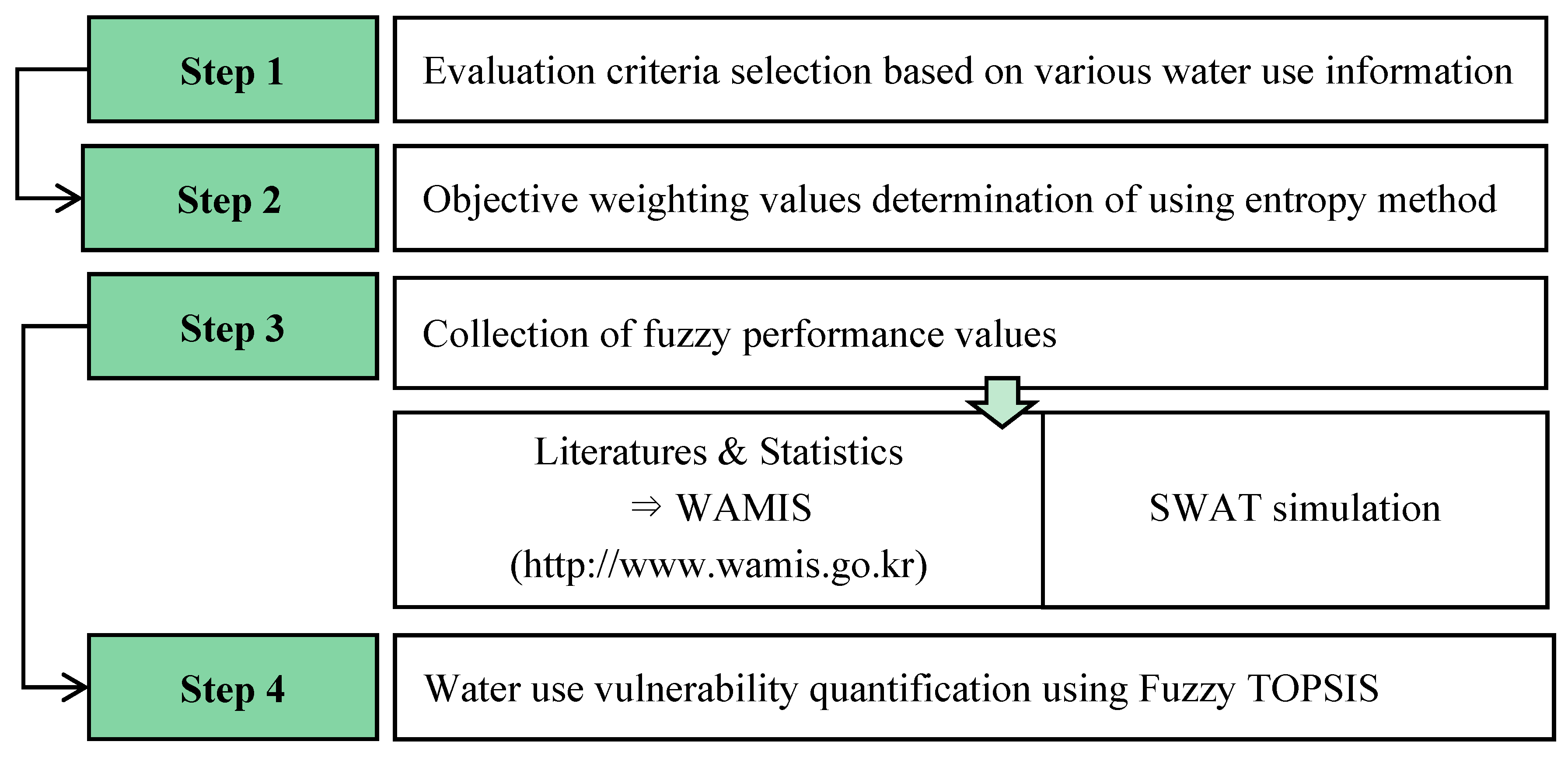
Using the IPCC vulnerability framework, the procedure used in this study consists of four steps as shown in Figure 1. The first step is to determine the evaluation criteria along with three aspects of climate exposure, sensitivity and adaptive capacity. The second step is to derive the objective weighting values using the Shannon entropy method. The third step is to collect fuzzy performance values obtained from Water Management Information System (WAMIS) and results of SWAT simulation. The final step is to quantify the water use vulnerability using Fuzzy TOPSIS coupled with entropy weights and rank all study basins.

Figure 1. Procedure for water use vulnerability assessment used in this study.

Figure 1. Procedure for water use vulnerability assessment used in this study.

2.2. Hydrological Model

The ArcView Interface of SWAT 2000 (AVSWAT2000) is a river basin model developed by the U.S. Department of Agriculture (USDA) Agricultural Research Service of Backland Research Center in Texas. SWAT can predict the impact of land management practices on water, sediment yield and non-point source pollution in large, complex watersheds [16]. The present study focuses solely on the hydrological component of the model.

The SWAT model uses many physical algorithms to estimate runoff. Using data such as precipitation, soil properties, topography, and land cover, the model calculates the runoff using the SCS curve number method [6]. According to land use map and soil data, SWAT can divide the watershed into Hydrologic Response Units (HRUs). The entire basin is divided into many smaller sub-basins by selecting points on the stream network that act as each individual outlet. The response of each HRU in terms of water, sediment, nutrient, and pesticide transformations is determined individually, and then aggregated at the sub-basin level. The discharges are routed to the associated reach and to the catchment outlet through the channel network [7]. The hydrological component of SWAT is based on the following water balance equation [17]:

$$S{W}_t=S{W}_0+{\displaystyle \sum }_{i=1}^t(R_i-Q_{surf}-E{T}_i-W_{seep}-Q_{gw})$$

(1)

where $S{W}_t$ is the final soil water content (mm), $S{W}_0$ is the initial soil water content on day i (mm), t is the time (days), $R_i$ is the amount of precipitation on day i (mm), $Q_{surf}$ is the amount of surface runoff on day i (mm), $E{T}_i$ is the amount of evapotranspiration on day i (mm), $W_{seep}$ is the amount of water entering the vadose zone from the soil profile on day i (mm), and $Q_{gw}$ is the amount of return flow on day i (mm).

2.3. Calibration and Uncertainty Analysis

The objectives of SWAT-CUP are: (1) to integrate various calibration/uncertainty analysis procedures for SWAT in one user interface; (2) to make the calibrating procedure easy to use for students and professional users; (3) to make the learning of the programs easier for the beginners; (4) to provide a faster way to do the time consuming calibration operations and standardize calibration steps; and (5) to add extra functionalities to calibration operations such as creating graphs of calibrated results, data comparison, etc. The program is written in C# programming platform. The SWAT-CUP to calibrate parameters has 5 programs, consisting of Sequential Uncertainty Fitting ver. 2 (SUFI-2), Generalized Likelihood Uncertainty Estimation (GLUE), Parameter Solution (ParaSol), Particle Swarm Optimization (PSO), and Markov Chain Monte Carlo (MCMC).

2.4. Fuzzy TOPSIS Coupled with Entropy

This study used fuzzy TOPSIS technique to quantify vulnerability in South Korea. This method was extended from TOPSIS to solve decision-making problems with uncertain data [18,19]. A fuzzy set has been introduced by [20] for handling uncertainty inherent in decision-making process. Fuzzy TOPSIS uses linguistic variables and fuzzy numbers, as opposed to crisp, to aggregate the subjective assessment of decision maker about various problems and validity of alternative candidate versus selection evaluation criteria to obtain the final scores-fuzzy validity indices. In this sense fuzzy set theory is certainly one of the theories which can be used to model the specific types of uncertainty under specific types of circumstances. It might then compete with other theories, but it might also be the most appropriate way to describe this phenomenon for well-specified situations [21]. A fuzzy set is a general form of a crisp set. A TFN belongs to the closed interval 0 and 1, which 1 addresses full membership and 0 expresses non-membership. It is often convenient to work with TFNs because they are relatively simple to compute and are useful in representing and processing information in a fuzzy environment [22]. A TFN, ${\tilde{X}}_{ij}$, can be defined by a triplet $(l, m, u)$. The membership function ${\tilde{X}}_{ij}$ is defined as:

$${\tilde{X}}_{ij}(x)=\{\begin{array}{c}0, x\le l\\ \begin{array}{c}\frac{x-l}{m-l}, l\le x\le m\\ \begin{array}{c}\frac{u-x}{u-m}, m\le x\le u\\ 0, \text{otherwise}\end{array}\end{array}\end{array}$$

(2)

The TOPSIS method was initiated for solving a multiple attribute decision making problem with no articulation of preference information [23]. The TOPSIS is based on the concept that the positive ideal solution (PIS) has the best level for all attributes considered, whereas the negative ideal solution (NIS) is the one with all the worst attribute values. A TOPSIS solution is defined as the alternative which is simultaneously farthest from the negative ideal solution and closest to the positive ideal solution.

Step 1. To consider fuzziness, as opposed to crisp data, values in $D$ (the performance matrix) and $W$ are presented as follow [24,25]:

$$\tilde{D}=[{\tilde{X}}_{ij}], \tilde{W}=[{\tilde{W}}_{ij}]$$

(3)

where ${\tilde{X}}_{ij}$ represents the fuzzy rating of basins $A_j$ with respect to criterion $C_i$, and ${\tilde{W}}_i$ is the fuzzy weight for criterion $C_i$.

In the absence of a reliable probability distribution function, an intuitively easy, effective, and commonly used approach to account for the uncertainty of the value of an unknown parameter is a TFN, ${\tilde{X}}_{ij}=(l, m, u)$. Therefore, the fuzzy performance matrix is formed by arraying columns of basins with rows of criteria, as shown below.

$$\tilde{D}=\left[\begin{array}{ccc}{\tilde{X}}_{11}& \cdots & {\tilde{X}}_{1n}\\ ⋮& \ddots & ⋮\\ {\tilde{X}}_{m1}& \cdots & {\tilde{X}}_{mn}\end{array}\right]$$

(4)

Step 2. The performance matrix should be normalized to convert the values into a common dimensionless unit for the comparison. The normalized performance ${\tilde{x}}_{ij}$ can be obtained using the following transformation formula. When the evaluation indicators are benefit criteria, normalization of the decision matrix can be expressed as Equation (5). Otherwise, the evaluation indicators are cost criteria, the calculations for normalization are as Equation (6):

$$\tilde{r}=(\frac{l}{c_i^{+}},\frac{m}{c_i^{+}},\frac{u}{c_i^{+}})$$

(5)

$$\tilde{r}=(\frac{a_i^{-}}{u},\frac{a_i^{-}}{m},\frac{a_i^{-}}{l})$$

(6)

where $c_i^{+}={\max }_j{c}_{ij}$, $a_i^{-}={\min }_j{a}_{ij}$, and ${\tilde{r}}_{ij}$ represents the normalized performance of $A_j$ with respect to attribute $C_j$.

The matrix form of ${\tilde{r}}_{ij}$ is given as follows:

$$\tilde{r}=[{\tilde{r}}_{ij}]$$

(7)

Step 3. This method provides objective weights with which to solve the uncertainty because it uses only the objective information.

To apply the entropy method suggested [26], this study constructed an original indicator value matrix:

$$\tilde{D}={(X_{ij})}_{m\times n}$$

(8)

where m and n represent the basins and the evaluating indicators, respectively. Because the evaluating indicators have different units, a normalization method is required to integrate the evaluation index. A standardized normalization matrix can be obtained as follows:

$$r_{ij}=\frac{X_{ij}}{{{\displaystyle \sum }}_{i=1}^m{X}_{ij}}$$

(9)

where $i=1,2,\cdots ,m$, $j=1,2,\cdots ,n$.

The uncertainty and entropy are smaller if a relatively large amount of information is available and vice versa [27]. The entropy is defined as follows:

$$r_{ij}=\frac{X_{ij}}{{{\displaystyle \sum }}_{i=1}^m{X}_{ij}}$$

(9)

$$H_i=-k{{\displaystyle \sum }}_{j=1}^n{f}_{ij} \text{log}{f}_{ij}$$

(10)

where $k=\frac{1}{\text{log}m}$ and $f_{ij}=\frac{r_{ij}}{{{\displaystyle \sum }}_{j=1}^n{r}_{ij}}$ when $f_{ij}=0, f_{ij}=\text{log}{f}_{ij}=0$.

Finally, the entropy weight of the i-th evaluating indicator is determined as

$${\tilde{W}}_i=\frac{1-H_i}{{{\displaystyle \sum }}_{i=1}^m(1-H_i)}$$

(11)

where $0\le {\tilde{W}}_i\le 1, {\displaystyle \sum }_i^m{\tilde{W}}_i=1$.

Step 4. By multiplying the performance matrix, ${\tilde{r}}_{ij}$, by its associated weights, $\tilde{W}$, the weighted performance matrix, $\tilde{V}$, is obtained as:

$$\tilde{V}=\tilde{r}\otimes \tilde{W}$$

(12)

Step 5. Calculating the distances of alternative $A_j$ to the ideal and anti-ideal alternatives, the fuzzy ideal weight distance is defined as follows:

$$d_j^{+}={[{{\displaystyle \sum }}_{i=1}^m{(d({\tilde{r}}_{ij}^{\tilde{w}},{\tilde{r}}_{ij}^{{+}^{\tilde{w}}}))}^q]}^{\raisebox{1ex}{$1$}\!\left/ \!\raisebox{-1ex}{$q$}\right.}$$

(13)

$$d_j^{-}={[{{\displaystyle \sum }}_{i=1}^m{(d({\tilde{r}}_{ij}^{\tilde{w}},{\tilde{r}}_{ij}^{{-}^{\tilde{w}}}))}^q]}^{\raisebox{1ex}{$1$}\!\left/ \!\raisebox{-1ex}{$q$}\right.}$$

(14)

where ${\tilde{R}}^w=[{\tilde{r}}_{ij}^w]$ is the weighted performance value of alternative $A_j$ with regard to criterion $C_i$.

Step 6. The ref. [28] proposed a multi-objective fuzzy pattern recognition model to provide the global evaluation for every alternative with respect to all criteria. According to the maximum principle of membership degree, one can select the desired alternative from n available alternatives. Then, the optimum membership degree of each alternative is defined as:

$$C^{*}=\frac{{(d_j^{-})}^2}{{(d_j^{+})}^2+{(d_j^{-})}^2}$$

(15)

3. Descriptions of Study Regions

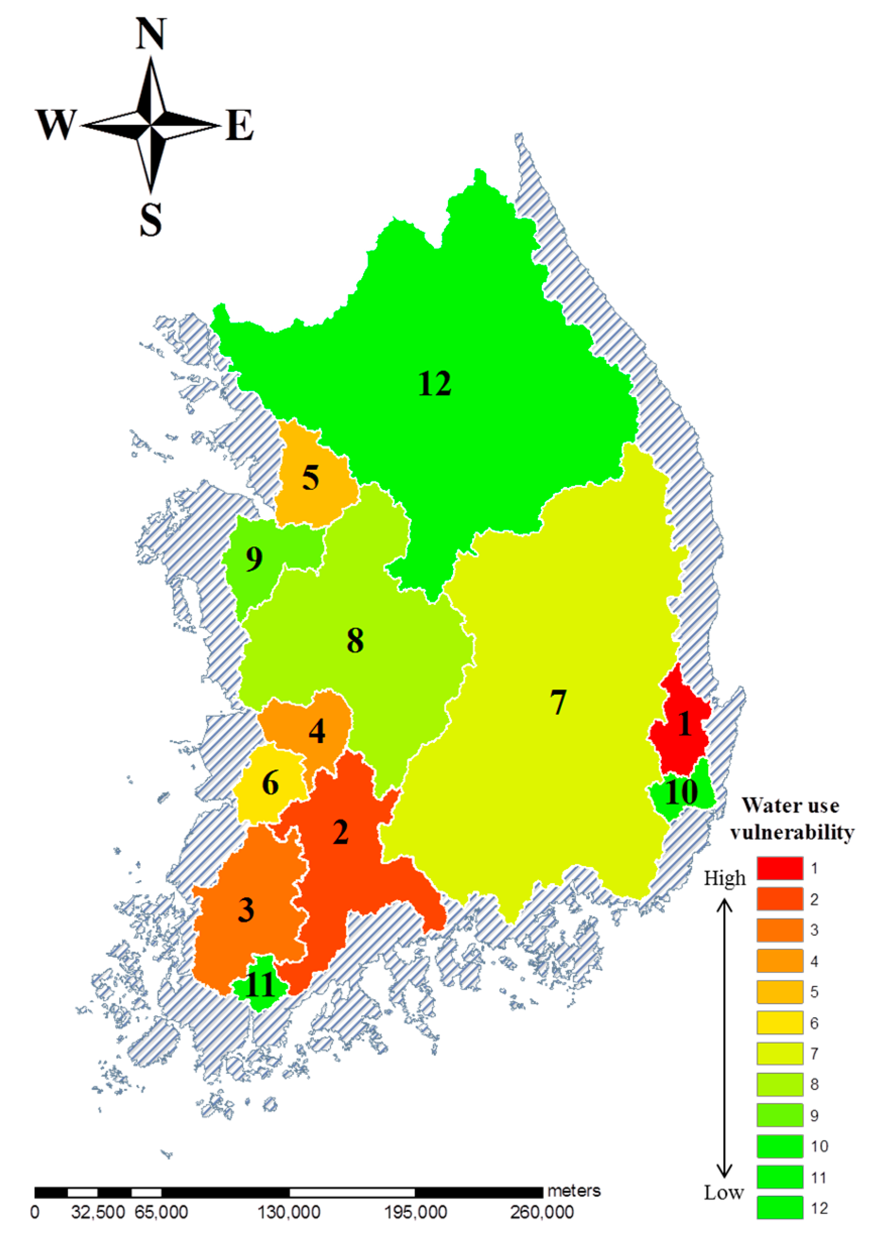
This study was applied to 12 major basins covering 88% territory of South Korea. They are all connected to three oceans adjacent to Korea peninsula. The study area and the characteristics of 12 basins are presented in Figure 2 and Table 1. 12 basins can be divided into two groups according to their areas, A1, A3, A5, A6, and A10 are five large river basins and the other seven (A2, A4, A7, A8, A9, A11, and A12) are medium-sized.

South Korea has a population of almost 51 million. About 68% of total population in South Korea resides in the study region. Especially, about 36% and 12% reside in the Han River basin (A1) and the Nakdong River basin (A10) while the smallest people reside in A7. There are six basins (A1, A2, A3, A5, A8, and A10) over one million residents.

Each basin contains a number of sub-basins as shown in the final column of Table 1. They were determined based on their DEMs and tributaries. This division was used to the SWAT formulation.

Figure 2. Description of the study area.

Figure 2. Description of the study area.

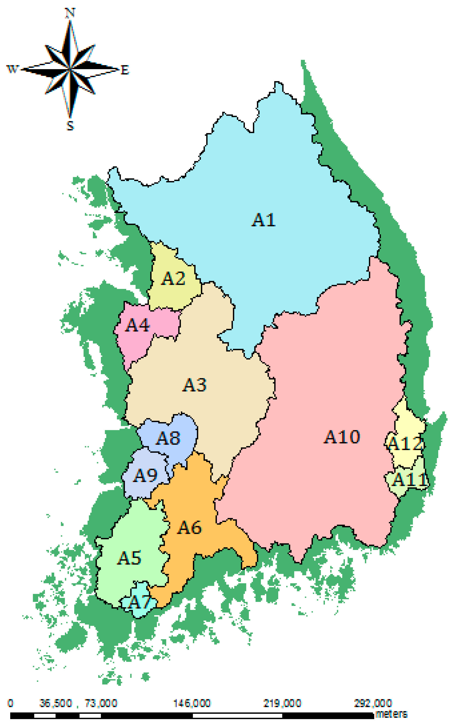
Table 1. Basin information of the study basins.

Name of Basin	Symbol	Basin Area (km2)	Population (Persons)	Population Density (Persons/km2)	Number of Sub-Basins
Han River	A1	34,428.10	18,366,766	533.5	17
Ansung River	A2	1658.66	1,834,349	1105.9	18
Geum River	A3	9914.02	3,060,877	308.7	14
Sapgyo River	A4	1668.39	638,312	382.6	16
Youngsan River	A5	3469.58	1,725,070	497.2	8
Seomjin River	A6	4914.32	319,614	65.0	9
Tamjin River	A7	505.52	42,161	83.4	4
Mangyung River	A8	1405.60	1,105,822	786.7	13
Dongjin River	A9	1117.53	240,685	215.4	8
Nakdong River	A10	23,690.32	6,417,380	270.9	22
Taehwa River	A11	660.86	725,310	1097.5	6
Hyeongsan River	A12	1139.99	382,497	335.5	9
Total		87,572.89	34,858,843	398.1	144

Table 1. Basin information of the study basins.

Name of Basin	Symbol	Basin Area (km2)	Population (Persons)	Population Density (Persons/km2)	Number of Sub-Basins
Han River	A1	34,428.10	18,366,766	533.5	17
Ansung River	A2	1658.66	1,834,349	1105.9	18
Geum River	A3	9914.02	3,060,877	308.7	14
Sapgyo River	A4	1668.39	638,312	382.6	16
Youngsan River	A5	3469.58	1,725,070	497.2	8
Seomjin River	A6	4914.32	319,614	65.0	9
Tamjin River	A7	505.52	42,161	83.4	4
Mangyung River	A8	1405.60	1,105,822	786.7	13
Dongjin River	A9	1117.53	240,685	215.4	8
Nakdong River	A10	23,690.32	6,417,380	270.9	22
Taehwa River	A11	660.86	725,310	1097.5	6
Hyeongsan River	A12	1139.99	382,497	335.5	9
Total		87,572.89	34,858,843	398.1	144

4. Hydrological Analysis

4.1. SWAT Formulation

The required data to build SWAT model consists of spatial and meteorological data. The spatial data includes DEM, and land use and soil maps. The meteorological data contains daily precipitation (mm), maximum and minimum temperatures (°C), solar radiation (MJ/m³day), average wind speed (m/s) and relative humidity (%) at the station of each basin, in addition to discharges at the gauges to calibrate and validate. A 30 m × 30 m DEM and 1:25,000 land use and soil maps were obtained from National Geographic Information Institute (NGII) of Ministry of Land, Infrastructure, and Transport (MOLIT) and Ministry of Environment (ME) and meteorological data from 1991 to 2014 was acquired from Korea Meteorological Administration (KMA).

4.2. Parameter Optimization Using SWAT-CUP

This study used the SUFI-2 algorithm in order to optimize parameters related to runoff. The 18 model parameters having their own physical and conceptual meanings were considered to the calibration as listed in Table 2. The SWAT hydrological parameters which are critical for the model performance are CN2, ALPHA_BF, GW_DELAY, GWQMN, GW_REVAP, REVAPMN, RCHRG_DP, ESCO, OV_N, SLSUBBSN, SOL_K, SOL_AWC, CH_N2, CH_K2, ALHPA_BNK, SMFMX, SMTMP and SFTMP. The ranges for parameter optimization used maximum and minimum values suggested by Absolute_SWAT_Values in SWAT-CUP model.

Table 2. Descriptions of selected parameters for SWAT calibration and validation [6].

Name of Parameter	Definition	Parameter Range
		Min	Max
r_CN2.mgt	SCS runoff curve number f	0	98
v_ALPHA_BF.gw	Baseflow alpha factor (days)	0	1
v_GW_DELAY.gw	Groundwater delay (days)	0	500
v_GWQMN.gw	Threshold depth of water in the shallow aquifer required for return flow to occur (mm)	0	5000
v_GW_REVAP.gw	Groundwater “revap” coefficient	0.02	0.2
v_REVAPMN.gw	Threshold depth of water in the shallow aquifer for “revap” to occur (mm)	0	500
v_RCHRG_DP.gw	Deep aquifer percolation fraction	0	1
v_ESCO.hru	Soil evaporation compensation factor	0	1
v_OV_N.hru	Manning’s “n” value for overland flow	0.01	30
v_SLSUBBSN.hru	Average slope length (m)	10	150
r_SOL_K.sol	Saturated hydraulic conductivity (mm/hr)	0	2000
r_SOL_AWC.sol	Available water capacity of the soil layer	0	1
v_CH_N2.rte	Manning’s “n” value for the main channel	−0.01	0.3
v_CH_K2.rte	Effective hydraulic conductivity in main channel alluvium (mm/hr)	−0.01	500
v_ALHPA_BNK.rte	Baseflow alpha factor for bank storage	0	1
v_SMFMX.bsn	Maximum melt rate for snow during year (occurs on summer solstice) (mm/day-°C)	0	20
v_SMTMP.bsn	Snow melt base temperature (°C)	−20	20
v_SFTMP.bsn	Snowfall temperature (°C)	−20	20

Table 2. Descriptions of selected parameters for SWAT calibration and validation [6].

Name of Parameter	Definition	Parameter Range
		Min	Max
r_CN2.mgt	SCS runoff curve number f	0	98
v_ALPHA_BF.gw	Baseflow alpha factor (days)	0	1
v_GW_DELAY.gw	Groundwater delay (days)	0	500
v_GWQMN.gw	Threshold depth of water in the shallow aquifer required for return flow to occur (mm)	0	5000
v_GW_REVAP.gw	Groundwater “revap” coefficient	0.02	0.2
v_REVAPMN.gw	Threshold depth of water in the shallow aquifer for “revap” to occur (mm)	0	500
v_RCHRG_DP.gw	Deep aquifer percolation fraction	0	1
v_ESCO.hru	Soil evaporation compensation factor	0	1
v_OV_N.hru	Manning’s “n” value for overland flow	0.01	30
v_SLSUBBSN.hru	Average slope length (m)	10	150
r_SOL_K.sol	Saturated hydraulic conductivity (mm/hr)	0	2000
r_SOL_AWC.sol	Available water capacity of the soil layer	0	1
v_CH_N2.rte	Manning’s “n” value for the main channel	−0.01	0.3
v_CH_K2.rte	Effective hydraulic conductivity in main channel alluvium (mm/hr)	−0.01	500
v_ALHPA_BNK.rte	Baseflow alpha factor for bank storage	0	1
v_SMFMX.bsn	Maximum melt rate for snow during year (occurs on summer solstice) (mm/day-°C)	0	20
v_SMTMP.bsn	Snow melt base temperature (°C)	−20	20
v_SFTMP.bsn	Snowfall temperature (°C)	−20	20

SWAT-CUP model includes sensitivity analysis of selected parameters for the calibration. The different results of the sensitivity analysis indicated that ALPHA_BNK was the most sensitive parameter for runoff in Ansung River, Geum River, Sapgyo River, Youngsan River, Seomjin River, Tamjin River, Mangyung River and Hyeongsan River. SLSUBBSN has been found to be the most sensitive parameter in Nakdong River and Dongjin River. CN2 and OV_N were sensitive for runoff in Han River and Taehwa River.

This study used two performance measures in order to evaluate how well data of optimized parameters fit: NSE and R² which is explained as follows:

The Nash-Sutcliffe coefficient (NSE) developed by [29] was used for the objective function and calculated as:

$$\text{NSE}=1-\frac{{{\displaystyle \sum }}_{t=1}^T{(q_{t, obs}-q_{t, sim})}^2}{{{\displaystyle \sum }}_{t=1}^T{(q_{t, obs}-\overline{q_{obs}})}^2}$$

(16)

where $q_{t, obs}$ and $q_{t, sim}$ are the observed and the simulated discharge, respectively, at time t, and $\overline{q_{obs}}$ is the averaged observed discharge.

The R² is the coefficient of determination and can be calculated using the Equation (15).

$$R^2=\frac{{[{{\displaystyle \sum }}_{t=1}^T(q_{t, obs}-\overline{q_{obs}})(q_{t, sim}-\overline{q_{sim}})]}^2}{{{\displaystyle \sum }}_{t=1}^T{(q_{t, obs}-\overline{q_{obs}})}^2{{\displaystyle \sum }}_{t=1}^T{(q_{t, sim}-\overline{q_{sim}})}^2}$$

(17)

where $q_{t, obs}$ and $q_{t, sim}$ are the observed and the simulated discharge, respectively, at time t, and $\overline{q_{obs}}$ and $\overline{q_{sim}}$ are the averages.

The NSE and R² can range from 0 to 1, where 0 indicates no correspondence and 1 correspond to a perfect match between the simulations and the observations. The ref. [30] suggested that model performance can be evaluated as “satisfactory” if NSE > 0.50. This study showed that the performance values are presented in Table 3. NSE values for the calibration and validation ranged from 0.51 to 0.92 and R² values ranged from 0.61 to 0.97. Discharge data is not enough to calibrate in the remaining basins. Therefore, based on sensitivity analysis, paramters of Ansung River and Sapgyo River used those of Tamjin River. Parameters of Youngsan River were applied in Geum River and Seomjin River.

Table 3. SWAT model performances in calibration and validation.

Watershed	Calibration		Validation
	Event		Event
	NSE	R2	NSE	R2
Han River	1 2009/01/01~2009/12/31		2014/01/01~2014/12/31
	0.81	0.85	0.51	0.62
Youngsan River	2008/01/01~2010/12/31		2013/01/01~2014/12/31
	0.83	0.91	0.81	0.90
Tamjin River	2009/01~2011/12		2012/01~2012/12
	0.64	0.78	0.53	0.78
Mangyung River	2010/01~2010/12		2014/01~2014/12
	0.79	0.88	0.76	0.79
Dongjin River	2008/01~2008/12		2011/01~2011/12
	0.55	0.61	0.51	0.63
Nakdong River	2011/01/01~2011/12/31		2014/01/01~2014/12/31
	0.81	0.89	0.53	0.87
Taehwa River	2012/01~2012/12		2014/01~2014/12
	0.51	0.76	0.89	0.91
Hyeongsan River	2009/01~2009/12		2014/01~2014/12
	0.88	0.93	0.92	0.97

Table 3. SWAT model performances in calibration and validation.

Watershed	Calibration		Validation
	Event		Event
	NSE	R2	NSE	R2
Han River	1 2009/01/01~2009/12/31		2014/01/01~2014/12/31
	0.81	0.85	0.51	0.62
Youngsan River	2008/01/01~2010/12/31		2013/01/01~2014/12/31
	0.83	0.91	0.81	0.90
Tamjin River	2009/01~2011/12		2012/01~2012/12
	0.64	0.78	0.53	0.78
Mangyung River	2010/01~2010/12		2014/01~2014/12
	0.79	0.88	0.76	0.79
Dongjin River	2008/01~2008/12		2011/01~2011/12
	0.55	0.61	0.51	0.63
Nakdong River	2011/01/01~2011/12/31		2014/01/01~2014/12/31
	0.81	0.89	0.53	0.87
Taehwa River	2012/01~2012/12		2014/01~2014/12
	0.51	0.76	0.89	0.91
Hyeongsan River	2009/01~2009/12		2014/01~2014/12
	0.88	0.93	0.92	0.97

4.3. Runoff Simulation

Runoffs for 12 basins were simulated using the optimized parameters. This study derived total runoffs and runoff depths of 12 study basins as shown in Figure 3. The values were averaged from 1991 to 2014.

The annual average runoffs of 12 basins could be arranged according to the amount as follows: A1 (229.36 m³/s), A10 (210.32 m³/s), A3 (91.11 m³/s), A6 (56.19 m³/s), A5 (47.18 m³/s), A12 (13.17 m³/s), A2 (12.05 m³/s), A8 (11.90 m³/s), A4 (9.78 m³/s), A9 (5.94 m³/s), A7 (4.39 m³/s), and A11 (3.90 m³/s). In case of runoff, A1 was the maximum whereas A11 was the minimum among 12 basins.

Additionally, annual runoff depths were calculated because total runoffs are highly influenced by basin area. The ranking was determined as follows: A6 (1188.32 mm), A7 (1131.14 mm), A11 (1084.85 mm), A10 (1040.58 mm), A2 (1030.48 mm), A5 (1015.35 mm), A3 (1004.41 mm), A8 (991.54 mm), A9 (940.62 mm), A4 (930.43 mm), A12 (926.84 mm), and A1 (675.78 mm). A6 was the maximum due to large precipitation and high runoff ratios. For runoff depth, the amount order is totally different from that of total runoffs.

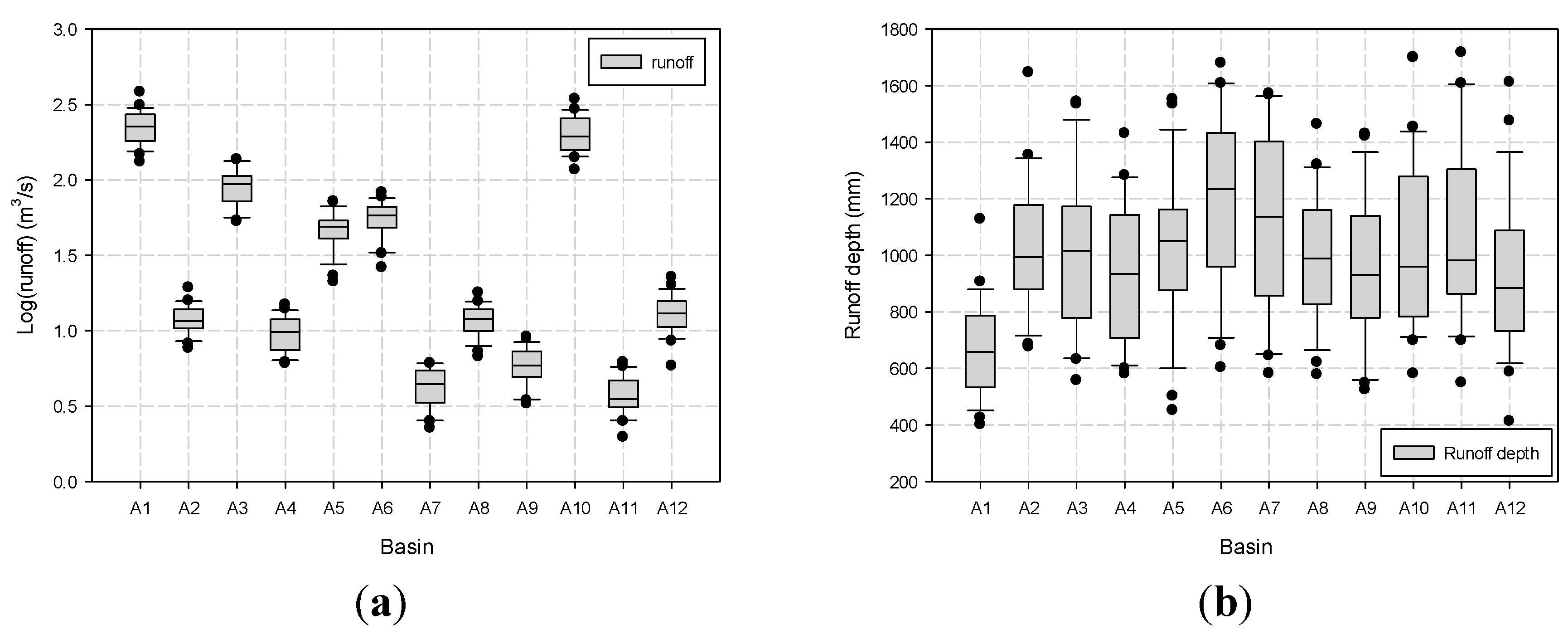
To find the variations of total runoffs and runoff depth, the Box-plot was drawn using 24-year data as shown in Figure 4. Total runoffs of large basins such as A1 and A10 have high variations. Runoff depths of A1 showed the smallest minimum runoffs while A6 and A7 showed the highest mean. A1, A5, and A12 showed the smallest minimum while A2, A6, A10 and A11 showed the highest maximum.

Figure 3. Simulated total runoff and runoff depth of the study regions. (a) Runoff (m³/s); (b) Runoff depth (mm).

Figure 3. Simulated total runoff and runoff depth of the study regions. (a) Runoff (m³/s); (b) Runoff depth (mm).

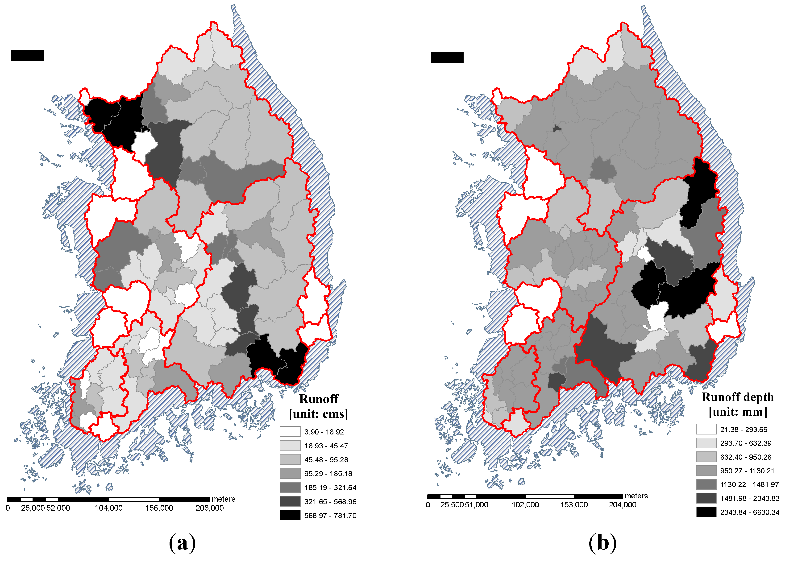
Figure 4. Box-Plots of total runoffs and runoff depths (1991-2014). (a) Runoff (cms); (b) Runoff depth (mm).

Figure 4. Box-Plots of total runoffs and runoff depths (1991-2014). (a) Runoff (cms); (b) Runoff depth (mm).

5. Results

5.1. Determination of Indicators and Derivation of Their Objective Weighting Values

Water use vulnerability can be assessed in various ways including social, economic, and hydrological factors from 1991 to 2014. Therefore, it can be also approached by anthropogenic factors such as water demand as well as natural water availability of a river and water loss of a watershed. Three experts consisting two civil servants and a professor selected 15 evaluation criteria to account for climate exposure, sensitivity and adaptive capacity as shown in Table 4.

Table 4. Evaluation sub-indices and indicators for water use vulnerability and their TFNs of weighting values.

Criteria	Evaluation Sub-Index	TFNs of Weighting Value			Evaluation Indicator	TFNs of Weighting VALUE
		Lower Bound	A model (Typical) Value	Upper Bound		Lower Bound	A Model (Typical) Value	Upper Bound
Adaptive capacity	Social/Economic	0.055	0.088	0.316	Water supply distribution ratio (%)	0.004	0.029	0.044
					Groundwater development density (Number of groundwater development/km2)	0.197	0.257	0.388
					Number of civil servants related to sewage treatment (persons)	0.145	0.173	0.230
					Reservoir capacity of dam (km3)	0.185	0.324	0.328
					Number of dams in basin (Number of dams/km2)	0.153	0.269	0.272
Sensitivity	Water availability	0.294	0.477	0.530	Population density (people/km2)	0.088	0.097	0.117
					Household water consumption per watershed area (103 m3/s/km2)	0.078	0.080	0.083
					Industrial water usage per watershed area (103 m3/s/km2)	0.198	0.338	0.368
					Agriculture water usage per watershed area (103 m3/s/km2)	0.031	0.032	0.043
					Water supply per capita (m3/day/people)	0.002	0.003	0.003
Climate exposure	Hydrology (loss)	0.084	0.108	0.150	Evapotranspiration (mm)	0.754	0.764	0.794
					Percolation (mm)	0.206	0.236	0.246
	Hydrology (supply)	0.240	0.327	0.330	Runoff per area (m3/s/km2)	0.045	0.071	0.078
					Runoff per capita (m3/s/people)	0.915	0.922	0.941
					Water yield (mm)	0.007	0.007	0.014

Table 4. Evaluation sub-indices and indicators for water use vulnerability and their TFNs of weighting values.

Criteria	Evaluation Sub-Index	TFNs of Weighting Value			Evaluation Indicator	TFNs of Weighting VALUE
		Lower Bound	A model (Typical) Value	Upper Bound		Lower Bound	A Model (Typical) Value	Upper Bound
Adaptive capacity	Social/Economic	0.055	0.088	0.316	Water supply distribution ratio (%)	0.004	0.029	0.044
					Groundwater development density (Number of groundwater development/km2)	0.197	0.257	0.388
					Number of civil servants related to sewage treatment (persons)	0.145	0.173	0.230
					Reservoir capacity of dam (km3)	0.185	0.324	0.328
					Number of dams in basin (Number of dams/km2)	0.153	0.269	0.272
Sensitivity	Water availability	0.294	0.477	0.530	Population density (people/km2)	0.088	0.097	0.117
					Household water consumption per watershed area (103 m3/s/km2)	0.078	0.080	0.083
					Industrial water usage per watershed area (103 m3/s/km2)	0.198	0.338	0.368
					Agriculture water usage per watershed area (103 m3/s/km2)	0.031	0.032	0.043
					Water supply per capita (m3/day/people)	0.002	0.003	0.003
Climate exposure	Hydrology (loss)	0.084	0.108	0.150	Evapotranspiration (mm)	0.754	0.764	0.794
					Percolation (mm)	0.206	0.236	0.246
	Hydrology (supply)	0.240	0.327	0.330	Runoff per area (m3/s/km2)	0.045	0.071	0.078
					Runoff per capita (m3/s/people)	0.915	0.922	0.941
					Water yield (mm)	0.007	0.007	0.014

Water supply distribution ratio, groundwater development density, number of civil servants, reservoir capacity of dam and dam density affecting the positive impacts on adaptive capacity were selected and checked their data availability. In addition, population density, household water consumption, industrial and agriculture water usages per unit area and water supply capita were chosen to the evaluation criteria for sensitivity. Climate exposure criteria can be determined from the results of SWAT simulation such as evapotranspiration and percolation as water loss and runoff depth, runoff per capita and water yield as water supply.

The relative importance on each indicator can be diversely derived depending on decision makers. Therefore, Shannon’s entropy method was used to determine the objective weighing values. Then, this study derived the fuzzified-entropy weights as shown in Table 4. The lower bounds of entropy-based weights for water availability were considerably higher than the others. In the weights of model values and upper bounds, indicators for water availability had also higher weights than the others. The indicators, such as industrial water usage per area, evapotranspiration, and runoff per capita have the highest weights in all TFNs. Their indicators were the most influential to the each index. Especially, runoff per capita is the highest weights in all bounds.

5.2. Fuzzification of Input Data

Datasets of social/economic and water availability were obtained from WAMIS [31] operated by MLTMA and the hydrology data were acquired from SWAT simulation. Because all data of 12 basins have 24 annual values from 1991 to 2014, this study used TFNs to reduce the uncertainty on the annual variations.

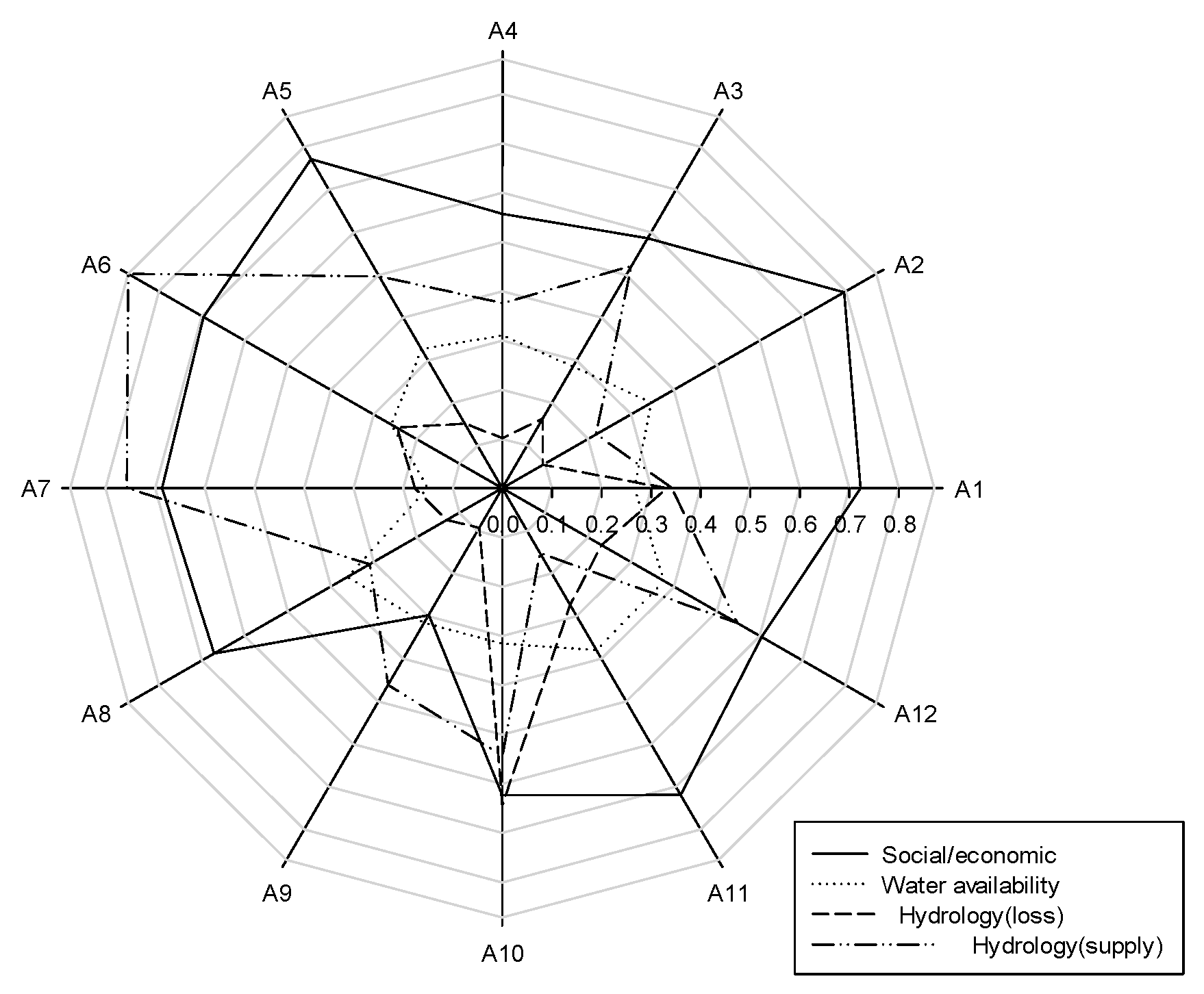
As stated section 2.4, the normalized performance matrix was constructed to convert the values into the dimensionless form for the calculation. This study used two normalization methods of “benefit-type” and “cost-type” according to the data characteristics. As shown Figure 5, the normalized decision matrix is fuzzified using TFNs. Figure 6 showed the influence of each sub-index was calculated. It presents the influential degrees for social/economic, water availability, water loss and water supply, respectively. As a result, water loss has less influential than the others. Especially, A6 and A11 and A12 were largely impacted in evaluation indicators belonging to water supply and availability indicators. Then the normalized fuzzy decision matrix was combined with the entropy weights using Equation (11).

Figure 5. TFNs of performance values of 12 basins for four evaluation sub-indices. (a) Social/economic index; (b) Water availability index; (c) Hydrology (loss) index; (d) Hydrology (supply) index.

Figure 5. TFNs of performance values of 12 basins for four evaluation sub-indices. (a) Social/economic index; (b) Water availability index; (c) Hydrology (loss) index; (d) Hydrology (supply) index.

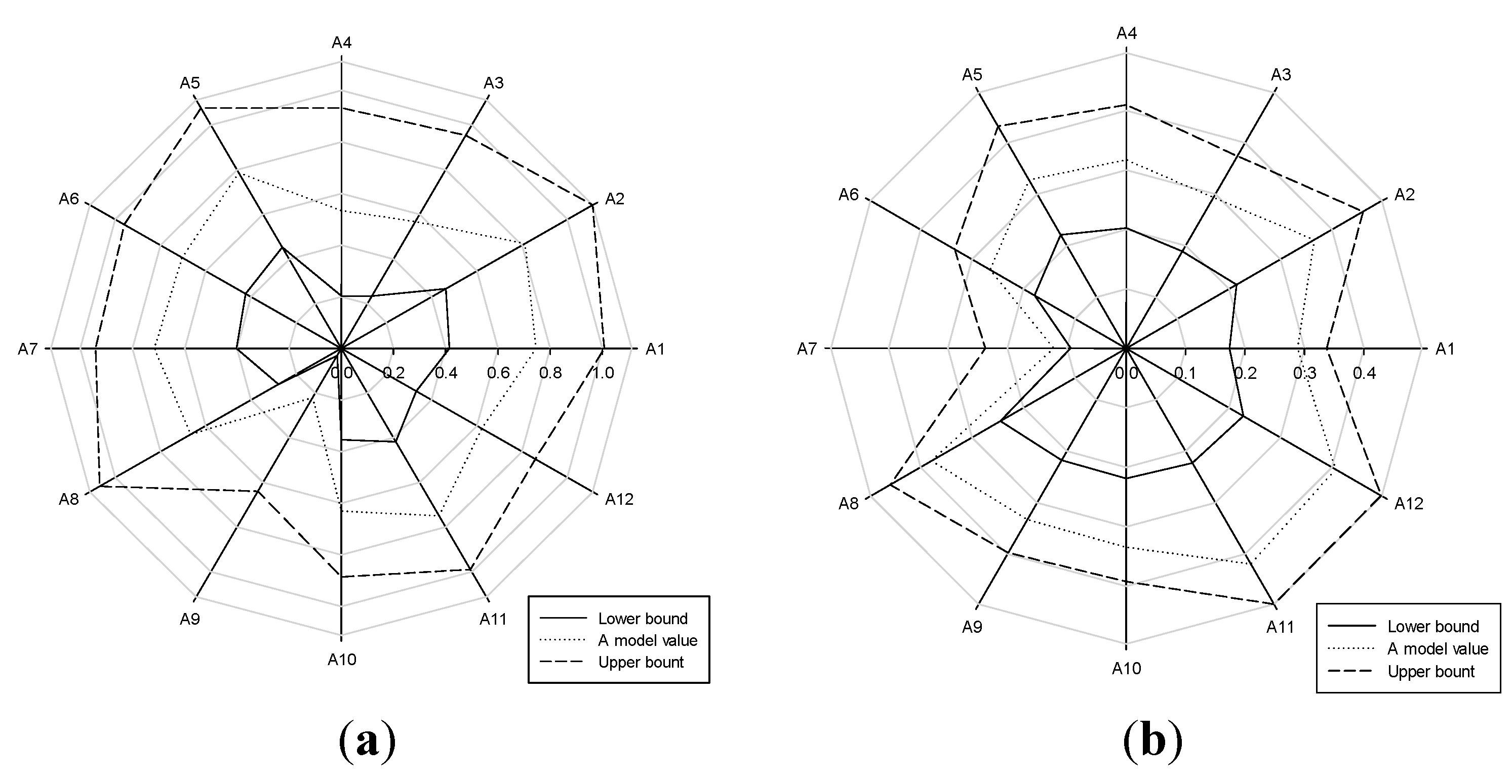
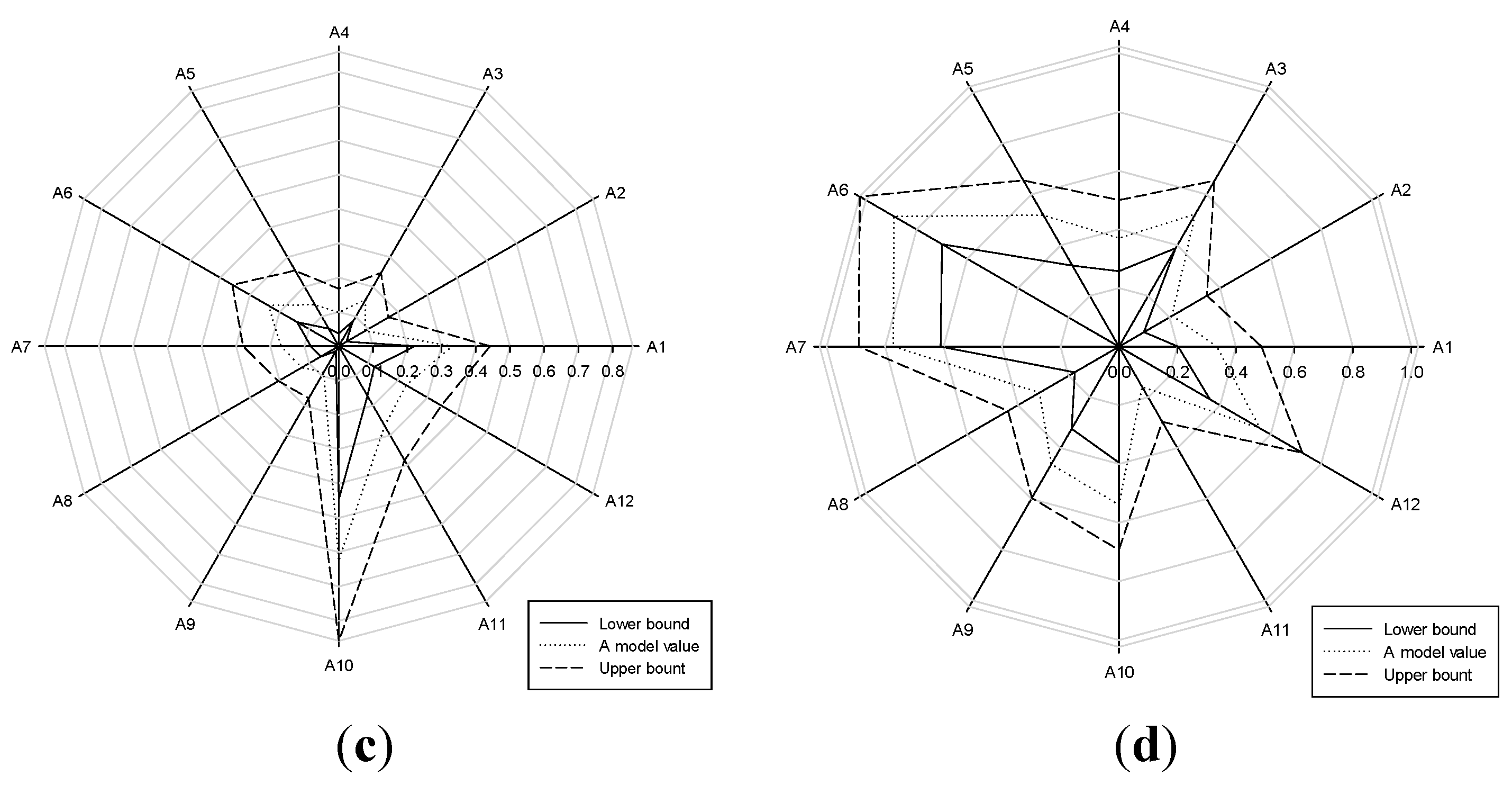
Figure 6. TFNs of performance values of 12 basins.

Figure 6. TFNs of performance values of 12 basins.

5.3. Water Use Vulnerability Assessment of South Korea

To apply the fuzzy TOPSIS method, fuzzy positive ideal solution (FPIS) and fuzzy negative ideal solution (FNIS) of all study basins were calculated as shown in Table 5. All relative closeness as shown in Table 6, were derived by combining FPIS and FNIS with all performance TFNs as presented in equation. (13). As a result, the ranking of water use vulnerability is as follows: A12 (Hyeongsan River) > A6 (Seomjin River) > A5 (Youngsan River) > A8 (Mangyung River) > A2 (Ansung River) > A9 (Dongjin River) > A10 (Nakdong River) > A3 (Geum River) > A4 (Sapgyo River) > A11 (Taehwa River) > A7 (Tamjin River) > A1 (Han River). They are summarized in a graphical form as shown in Figure 7. A12 was the most vulnerable and A6 and A5 were the next most vulnerable among 12 basins whereas A1 is the most anti-vulnerable (or stable).

Table 5. Values of FPIS and FNIS in this study.

FPIS/FNIS	Social/Economics	Water Availability	Hydrology (Loss)	Hydrology (Supply)
A*	0.0016	0.0553	0.0016	0.0004
A−	0.3159	0.5305	0.1502	0.3298

Table 5. Values of FPIS and FNIS in this study.

FPIS/FNIS	Social/Economics	Water Availability	Hydrology (Loss)	Hydrology (Supply)
A*	0.0016	0.0553	0.0016	0.0004
A−	0.3159	0.5305	0.1502	0.3298

Table 6. Relative closeness and rankings of 12 basins.

Symbol	d+	d−	C*	Ranking
A1	0.51	0.90	0.36	12
A2	0.62	0.86	0.42	5
A3	0.58	0.84	0.41	8
A4	0.58	0.86	0.40	9
A5	0.64	0.81	0.44	3
A6	0.65	0.78	0.45	2
A7	0.53	0.88	0.37	11
A8	0.62	0.84	0.42	4
A9	0.60	0.84	0.42	6
A10	0.58	0.83	0.41	7
A11	0.58	0.89	0.39	10
A12	0.67	0.79	0.46	1

Table 6. Relative closeness and rankings of 12 basins.

Symbol	d+	d−	C*	Ranking
A1	0.51	0.90	0.36	12
A2	0.62	0.86	0.42	5
A3	0.58	0.84	0.41	8
A4	0.58	0.86	0.40	9
A5	0.64	0.81	0.44	3
A6	0.65	0.78	0.45	2
A7	0.53	0.88	0.37	11
A8	0.62	0.84	0.42	4
A9	0.60	0.84	0.42	6
A10	0.58	0.83	0.41	7
A11	0.58	0.89	0.39	10
A12	0.67	0.79	0.46	1

Figure 7. Summary of water use vulnerability ranking.

Figure 7. Summary of water use vulnerability ranking.

5.4. Comparative Analysis of Water Use Vulnerability

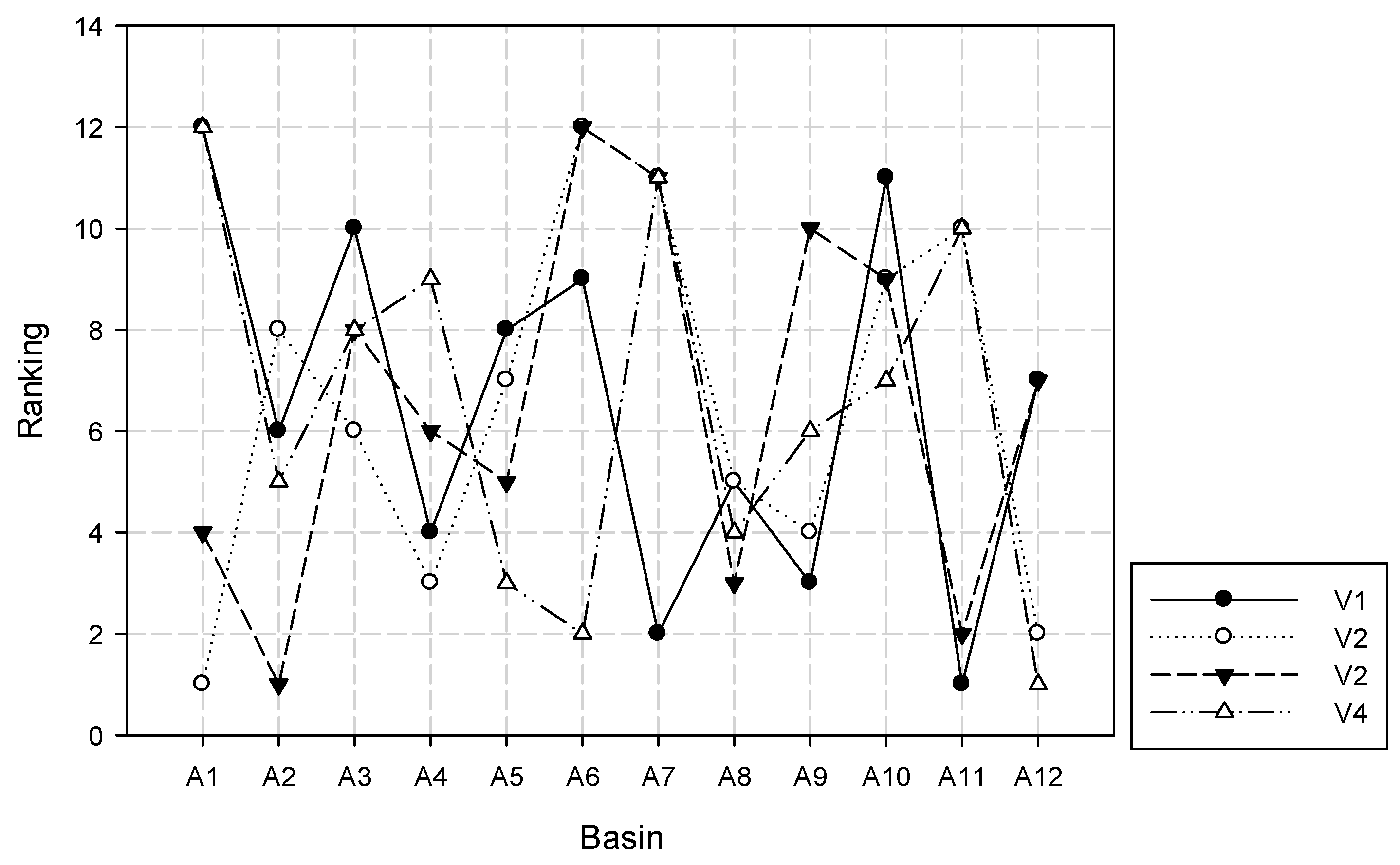
This study compared the water use vulnerability ranking (V4) to those from total runoff (V1), runoff depth (V2) and runoff per capita (V3) as shown in Figure 8. As a result, four rankings are clearly different. It is concluded that A1 is not vulnerable in total runoff while runoff depth and runoff per capita of A1 are very low. Also, A6 is not vulnerable in runoff depth and per capita whereas this is vulnerable in the water use vulnerability assessment. In other words, A1 and A7 show the opposite trend of high vulnerability. In terms of runoff, A4, A8 and A11 are relatively vulnerable than other basins. On the other hand, those three basins showed low vulnerability in water use vulnerability. Also, A6 and A5 showed very high vulnerability but are anti-vulnerable in terms of V1, V2 and V3.

Figure 8. Comparison of water use vulnerability rankings.

Figure 8. Comparison of water use vulnerability rankings.

To find the quantitative associations between rankings, the Spearman rank correlation coefficients were calculated in this study as shown in Table 7. The value of R always lies between −1 and +1, with these two extremes indicating a perfect association between the parameters. Here, the plus sign indicates identical rankings and the minus sign indicates reverse rankings. R= −1 represents perfect disagreement between the ranks. When R is close to zero, there is no association between the rankings of the alternatives [32]. As described in the above, the correlations are very low. Therefore, it can be certainly stated that any single-indicator values cannot determine the water use vulnerability of large areas. Furthermore, it should be required to consider the annual variations using TFNs. It can reduce the uncertainty inherent in quantifying water use vulnerability.

Table 7. Spearman ranking correlations among results of four methods.

	Runoff	Runoff Depth	Runoff per Capita	Vulnerability Using Fuzzy Topsis
Runoff	1	−0.203	0.112	−0.147
Runoff depth	-	1	0.287	−0.035
Runoff per capita	-	-	1	−0.098
Vulnerability using fuzzy TOPSIS	-	-	-	1

Table 7. Spearman ranking correlations among results of four methods.

	Runoff	Runoff Depth	Runoff per Capita	Vulnerability Using Fuzzy Topsis
Runoff	1	−0.203	0.112	−0.147
Runoff depth	-	1	0.287	−0.035
Runoff per capita	-	-	1	−0.098
Vulnerability using fuzzy TOPSIS	-	-	-	1

6. Conclusions

This study used the objective framework to assess the water use vulnerability using fuzzy TOPSIS coupled with the Shannon entropy method. It was applied to the 12 major basins covering 88% area of South Korea. SWAT model was applied to simulate the hydrological components and SWAT-CUP was used to calibrate and validate SWAT’s parameters. In terms of climate exposure, sensitivity and adaptive capacity, 15 indicators for water use vulnerability were proposed by three experts and their relative importance are objectively determined using the entropy method.

As a result, the ranking of water use vulnerability is derived as follows: A12 (Hyeongsan River) > A6 (Seomjin River) > A5 (Youngsan River) > A8 (Mangyung River) > A2 (Ansung River) > A9 (Dongjin River) > A10 (Nakdong River) > A3 (Geum River) > A4 (Sapgyo River) > A11 (Taehwa River) > A7 (Tamjin River) > A1 (Han River). Also, it was compared to the three rankings obtained from total runoff, runoff depth, and runoff per capita. Then, the Spearman rank correlations among four results showed very low values between any rankings. Therefore, it can be certainly stated that any single-indicator values cannot decide the water use vulnerability of large areas. Furthermore, it should be required to consider the annual variations using TFNs. It can reduce the uncertainty inherent in quantifying water use vulnerability.

In the future, this study will be utilized in the sustainable water resources management and also used to the climate change vulnerability assessment for the Korea peninsula.

References

- Oki, T.; Kanae, S. Global hydrological cycles and world water resources. Science 2006, 5790, 1068–1072. [Google Scholar] [CrossRef] [PubMed]
- IPCC. Contribution of Working Group II to the Fourth Assessment Report of the Intergovernmental Panel on Climate Change; Parry, M.L., Canziani, O.F., Palutikof, J.P., van der Linden, P.J., Hanson, C.E., Eds.; Cambridge University Press: Cambridge, UK, 2007. [Google Scholar]
- Falkenmark, M. Freshwater as shared between society and ecosystems: From divided approaches to integrated challenges. Philos. T. Roy. Soc. Lond. 2003, 358, 2037–2049. [Google Scholar] [CrossRef] [PubMed]
- Arnold, J.G.; Srinivasan, R.; Muttiah, R.; Williams, J. Large area hydrologic modeling and assessment part I: Model development1. J. Am. Water Resour. Assoc. 1998, 34, 73–89. [Google Scholar] [CrossRef]
- EAWAG. SWAT-CUP 2012: SWAT Calibration and Uncertainty Programs—A User Manual; Swiss Federal Institute of Aquatic Science and Technology, Eawag: Duebendorf, Switzerland, 2013. [Google Scholar]
- Abbaspour, K.C. User Manual for SWAT-CUP, SWAT Calibration and Uncertainty Analysis Programs; Swiss Federal Institute of Aquatic Science and Technology, Eawag: Duebendorf, Switzerland, 2007; p. 93. [Google Scholar]
- Arnold, J.G.; Moriasi, D.N.; Gassman, P.W.; Abbaspour, K.C.; White, M.J.; Srinivasan, R.; Santhi, C.; Harmel, R.D.; van Griensven, A.; van Liew, M.W.; et al. SWAT: Model use, calibration, and validation. Trans. ASABE 2012, 55, 1494–1508. [Google Scholar] [CrossRef]
- Jun, K.S.; Chung, E.S.; Sung, J.Y.; Lee, K.S. Development of spatial water resources vulnerability index considering climate change impacts. Sci. Total Environ. 2011, 409, 5228–5242. [Google Scholar] [CrossRef] [PubMed]
- Lee, G.M.; Jun, K.S.; Chung, E.S. Integrated multi-criteria flood vulnerability approach using fuzzy TOPSIS and Delphi technique. Nat. Hazards Earth Syst. Sci. 2013, 13, 1293–1312. [Google Scholar] [CrossRef]
- Kim, Y.J.; Chung, E.S. Fuzzy VIKOR approach for assessing the vulnerability of the water supply to climate change and variability in South Korea. Appl. Math. Model. 2013, 37, 9419–9430. [Google Scholar] [CrossRef]
- Kim, Y.J.; Chung, E.S. Assessing climate change vulnerability with group multi-criteria decision making approaches. Clim. Change 2013, 121, 301–315. [Google Scholar] [CrossRef]
- Chung, E.S.; Won, K.J.; Kim, Y.J.; Lee, H.S. Water resources vulnerability characteristics by district’s population size in a changing climate using subjective and objective weights. Sustainability 2014, 6, 6141–6157. [Google Scholar] [CrossRef]
- Lee, G.M.; Jun, K.S.; Chung, E.S. Group decision-making approach for flood vulnerability identification using the fuzzy VIKOR method. Nat. Hazards Earth Syst. Sci. 2015, 15, 863–874. [Google Scholar] [CrossRef]
- IPCC. Climate Change 2001: Impacts, Adaptation Vulnerability. In Contribution of Working Group II to the Third Assessment Report of the Intergovernmental Panel on Climate Change; UNEP/WMO: Geneva, Switzerland, 2001. [Google Scholar]
- Adger, W.N. Vulnerability. Glob. Environ. Change 2006, 16, 268–281. [Google Scholar] [CrossRef]
- Neitsch, S.L.; Arnold, J.G.; Kiniry, J.R.; Srinivasan, R.; Williams, J.R. Soil and Water Assessment Tool, User Manual, Version 2000; Grassland, Soil and Water Research Laboratory: Temple, TX, USA, 2002. [Google Scholar]
- Ghaffari, G.; Keesstra, S.; Ghodousi, J.; Ahmadi, H. SWAT-simulated hydrological impact of land-use change in the Zanjanrood basin, northwest Iran. Hydrol. Proc. 2010, 24, 892–903. [Google Scholar] [CrossRef]
- Chung, E.S.; Kim, Y.J. Development of fuzzy multi-criteria approach to prioritize locations of treated wastewater use considering climate change scenarios. J. Environ. Manag. 2014, 146, 505–516. [Google Scholar] [CrossRef] [PubMed]
- Jun, K.S.; Chung, E.S.; Kim, Y.G.; Kim, Y.J. A fuzzy multi-criteria approach to flood risk vulnerability in South Korea by considering climage change impacts. Expert Syst. Appl. 2013, 40, 1003–1013. [Google Scholar] [CrossRef]
- Zadeh, L.A. Shadows of fuzzy sets. Probl. Transf. Inf. 1966, 2, 37–44. [Google Scholar]
- Zimmermann, H.J. Fuzzy Set Theory-and Its Applications; Springer: Heidelberg, Germany, 2001. [Google Scholar]
- Torlak, G.; Sevkli, M.; Zaim, S. Analyzing business competition by using fuzzy TOPSIS method: An example of Turkish domestic airline industry. Expert Syst. Appl. 2011, 38, 3396–3406. [Google Scholar] [CrossRef]
- Hwang, C.L.; Yoon, K. Multiple Attributes Decision Making Methods and Applications; Springer: Heidelberg, Germany, 1981. [Google Scholar]
- Afshar, A.; Marino, M.A.; Saadatpour, M.; Afsahr, A. Fuzzy TOPSIS multi-criteria decision analysis applied to Karun reservoirs system. Water Resour Manag. 2011, 25, 545–563. [Google Scholar] [CrossRef]
- Chen, C.T. Extensions of the TOPSIS for group decision-making under fuzzy environment. Fuzzy Sets Syst. 2000, 114, 1–9. [Google Scholar] [CrossRef]
- Shannon, C.E. A mathematical theory of communication. Bell Syst. Tech. J. 1948, 27, 379–423. [Google Scholar] [CrossRef]
- Yan, J.; Zhang, T.; Zhang, B.; Wu, B. Application of entropy weight fuzzy comprehensive evaluation in optimal selection of engineering machinery. In Proceedings of the 2008 International Colloquium on Computing, Communication, Control, and Management, Guangzhou, China, 3–4 August 2008; pp. 220–223.
- Zhou, H.C.; Wang, G.L.; Yang, Q. A multi-objective fuzzy recognition model for assessing groundwater vulnerability based on the DRASTIC system. Hydrol. Sci. 1999, 44, 611–618. [Google Scholar]
- Nash, J.E.; Sutcliffe, J.V. River flow forecasting through conceptual models. Part I: A discussion of principles. J. Hydrol. 1970, 10, 282–290. [Google Scholar] [CrossRef]
- Moriasi, D.N.; Arnold, J.G.; van Liew, M.W.; Bingner, R.L.; Harmel, R.D.; Veith, T.L. Model evaluation guidelines for systematic quantification of accuracy in watershed simulations. Trans. ASABE 2007, 50, 885–900. [Google Scholar] [CrossRef]
- WAMIS. Available online: http://wamis.go.kr/eng/ (accessed on 31 August 2015).
- Chung, E.S.; Lee, K.S. Identification of spatial ranking of hydrological vulnerability using multi-criteria decision making techniques: Case study of Korea. Water Resour. Manag. 2009, 23, 2395–2416. [Google Scholar] [CrossRef]
© 2015 by the authors; licensee MDPI, Basel, Switzerland. This article is an open access article distributed under the terms and conditions of the Creative Commons Attribution license (http://creativecommons.org/licenses/by/4.0/).