Probabilistic Cash Flow-Based Optimal Investment Timing Using Two-Color Rainbow Options Valuation for Economic Sustainability Appraisement

Abstract

This research determines the optimal investment timing using real options valuation to support decision-making for economic sustainability assessment. This paper illustrates an option pricing model using the Black-Scholes model applied to a case project to understand the model performance. Applicability of the project to the model requires two Monte Carlo simulations to satisfy a Markov process and a Wiener process. The position of project developers is not only the seller of products, but it is also the buyer of raw materials. Real options valuation can be influenced by the volatility of cash outflow, as well as the volatility of cash inflow. This study suggests two-color rainbow options valuation to overcome this issue, which is demonstrated for a steel plant project. The asymmetric results of the case study show that cash outflow (put option) influences the value of the steel plant project more than cash inflow (call option) does of which the discussion of the results is referred to a sensitivity analysis. The real options valuation method proposed in this study contributes to the literature on applying the new model, taking into consideration that investors maximize project profitability for economic sustainable development.

1. Introduction

Since the U.S. was hit by the Global Financial Crisis in 2008, the world economy has declined; a situation that continues to the present time. According to the Steel Statistical Yearbook, the steel industry has not been immune to this decline, making efficient and accurate project profitability of the upmost importance [1]. In this context, Korean steel companies have been seeking to open new markets through overseas business to ensure their economic sustainability. However, a new steel plant project engenders a large, fixed, and irreversible cost [2]. An investment in a steel plant project should be a very cautious decision. Market imperfections provide an important opportunities to create radical technologies and innovative business models based on sustainable entrepreneurship [3]. Especially, in order to succeed in sustainable entrepreneurship in the unstable market, enterprises should continuously develop. In other words, the development of enterprises is a continual success of investment. In order for investors to continue to invest successfully, it is necessary to predict the risks of investment projects and to identify sustainable investment opportunities. Therefore, it is important to consider the risks and opportunities together to find the optimal investment timing in project decisions due to the economic irreversibility [4,5].

The discounted cash flow (DCF) method is a long-used valuation method for steel plant projects. DCF is a method of measuring the future cash flows of a project by converting the gains into the present value (PV), and is currently the most widely used valuation method for decision making by investors [6]. However, DCF does not systematically reflect uncertainties caused by sudden changes in the environment. If any project cannot presently generate cash flow, but is highly likely to generate cash flow in the future, investors may miss a good opportunity due to DCF not reflecting this future potential inflow. In addition, DCF is limited in that it does not adequately evaluate option values that can flexibly determine investments for investors depending on the situation. A real options valuation (ROV), a method to overcome these shortcomings, is suitable for assessing the value of a project because it can estimate the value of business flexibility due to changes in the environment and consider future uncertainties.

Project developers are both the sellers of products and the buyers of raw materials. In other words, they are sensitive to the volatility of the price of products in terms of the sellers, and are sensitive to the volatility of the price of raw materials in terms of the buyers. Traditional ROV analyzed only one side of the seller or buyer [4,7,8,9,10,11,12,13,14,15,16]. In this paper, a steel plant project, which is a case study, is a large seller of steel products and a large buyer of iron ores and coal. In this case, the cash flow of the project is separated into cash inflow of the sellers and cash outflow of the buyers and applied to the model. Therefore, the major contribution of this study is to present a model that simultaneously considers both the seller of products and buyer of raw materials to solve this issue of the traditional ROV. This study also confirms the suitability of steel plant projects by applying an ROV that suits the characteristics of OPM. Then, the results of the model’s application to a case study of a steel plant project is described to verify that the cash outflow of the project should be considered. A sensitivity analysis is performed to check how differences between the volatilities of cash inflow and cash outflow affect the option value.

2. Literature Review

In economics, an asset price moves in a random walk, assuming an efficient market hypothesis [17]. In the efficient market hypothesis, the PV completely reflects the past record of asset prices, and the market reacts directly to the latest information about the asset. If these hypotheses are met, the asset price is said to follow the Markov process [18]. Over time, the variables that change uncertainly in the continuous time process follow the stochastic process. The process of changing these variables is called the Wiener process, which is a probability process with an annual mean of 0 and an annual variance of 1 [19]. In thermal physics, this process behaves similarly to the motion of a molecule due to the many small impacts from other molecules, and is called Brownian motion. An option provides investors with the right to buy or sell something until maturity at a specific contracted price depending on the type of option (call or put), but investors are not obliged to exercise this right [20]. The underlying assets for options include stocks, stock indices, interest rates, currencies, crude oil, insurance contracts, weather, and even real assets, such as projects. ROV dealing with the value of diverse projects through various option types has been actively researched, as are the following papers. The Black-Scholes model is common in the OPM [21]. The Black-Scholes partial differential equations can be derived using Ito’s lemma. Trigeorgis [22] focused on easily introducing an option to expand, contract, abandon, and defer projects through analysis of comprehensive industrial examples, such as raw material development, rural urban development, alternative business models, flexible production systems, and elsewhere. Lee et al. [23] used ROV as a solution to financial barriers to government guarantees in implementing green building projects. They measured ROV by estimating the value of the government guarantees for risks to uncertainties of that asset value. Lee et al. [24] obtained the ROV for a sequential investment in commercial energy retrofit projects on building performance risks as a case study. They also provided investors with advanced management knowledge of investments in performance risks with more accurate project information by assessing potential risks, barriers, and revenues. Zhao and Tseng [2] studied the ROV for an optimal infrastructure investment in preparation for the expansion of a public parking garage project. They identified the value of improving infrastructure flexibility for infrastructure expansion by applying ROV. Mayer and Kazakidis [25] acquired values for project capacity options and project shutdown options for a mine production system design and applied ROV to the investment decision process. Each type of ROV was only represented by a call or put option depending on the project situation of the ROV.

Studies using ROV to determine the optimal investment timing of projects have steadily developed. Trigeorgis [8] investigated the effects of competition on the optimal timing to start a project through an option pricing model (OPM). The author said that the presence of competitors can speed up a company’s planned investment and the expected preemptive competition is similar to dividends on options. Benaroch and Kauffman [10] analyzed the timing of the deployment of information technology projects and a range of issues associated with the application of ROV to problems in capital budgeting. The authors provided a formal rationale for the validity of the Black-Scholes model in relation to the capital budgeting methods that might be used to evaluate projects, and conducted sensitivity analyses to support verification. Kauffman and Li [12] developed a continuous-time probability model to determine the optimal timing for technologically controlled selection within the ROV framework. They also suggested that technology adopters should postpone their investments until the target technology dominates the market where the probability of achieving a critical mass reaches a threshold. Bøckman et al. [4] presented an ROV for choosing the optimal timing and capacity for small hydropower plants. They presented ROV along with continuous expansion of how to evaluate the small hydropower plant projects affected by uncertain electricity prices and suggested price limits to initiate the project. These studies have been conducted to evaluate the value of technology or business using ROV’s deferring option, and investigate optimal investment timing in various projects.

The abovementioned studies focused on inward project cash flow volatility only and did not consider outward cash flow volatility simultaneously. Odeyinka et al. [15] studied 26 identified significant risk factors for baseline forecasting of construction cost flow, and proposed a predictive mode for risk assessment. Maravas and Pantouvakis [16] conducted a study to calculate activity duration and cost through an uncertain project cash outflow based on the payment methods or the fluctuations in capital requirements. In a construction project, Hwee and Tiong [11] confirmed the influence of cash inflow and outflow on the sensitivity analysis, according to five factors: duration, over/under measurement risk, variation risk, material cost variances, predicted cash inflow, and cash outflow in progress. Kenley and Wilson [7] found that external cash flow is more relevant to the model than internal cash flow when forecasting net cash flows in a construction project. These studies emphasized the importance of predicting cash outflows rather than cash inflows in project implementation. However, they have common limitations. That is, these studies focus on the construction phase of the project, missing the valuation of the entire lifecycle project over several decades. In order to overcome these limitations, this paper performs the estimation and forecasting of cash inflow and cash outflow over several decades. The manufacturing enterprises fundamentally generate cash flows by constructing a factory, buying raw materials, operating a factory, and selling products. Factory construction, raw material purchase, and factory operation cause cash outflow, and product sales lead to cash inflow. In particular, prices of raw materials and products fluctuate with time. Both inward cash flow volatility and outward cash flow volatility are significant concerns in investment decisions. Therefore, this paper presents a model to consider both the volatility of cash inflows and cash outflows. The main component of cash inflow is the project’s revenue, which is the unit price multiplied by the sales volume. These studies considered ROV as a major factor in the volatility of unit prices and/or volatility of sales volumes. However, the volatility of cash outflow can also be a major part of the project’s value depending on the nature of the project.

The main components of cash outflow are capital expenditure (CAPEX) and operating expenditure (OPEX). CAPEX refers mainly to the initial investment cost of the project in a construction period. The volatility of CAPEX was identified through various cases of final project costs that differed from contracted project costs [9]. OPEX refers to the materials, labor, overhead, and other costs required in a business period. In particular, several studies addressed fluctuations in material costs [13,14,26]. Chen [13] conducted a significant study of inter-cluster and intra-cluster responses to the volatility of long-term behavior of raw material prices. Dwyer et al. [14] researched the volatility of various commodity prices, including steel products, on short-term price dynamics for financial investors based on long-term data. Jacks et al. [26] has used historical data since 1700 to analyze the impact of commodity price volatility on poor countries and found that commodity price volatility does not vary with output. Their papers used long-term price estimation and short-term price estimation through the volatility of raw material prices. Their claims focus on raw material prices themselves and need to take advantage of the forecasting part of the project value needed for the company's ongoing development. In this paper, we use the volatility that they claim in the estimation phase and further use the forecasting phase of ROV to evaluate the project value. To overcome the gap in the current literature [4,7,8,9,10,11,12,13,14,15,16] presented within this paper is the optimal investment timing by means of an ROV of two-color rainbow option, which can consider volatilities in both the cash inflow and cash outflow. Rainbow option valuation represents options whose payoff depends on the multiple underlying assets [27]. In other words, the value of the options is determined by the conditions and circumstances of the underlying assets.

3. Optimal Investment Timing for a Project

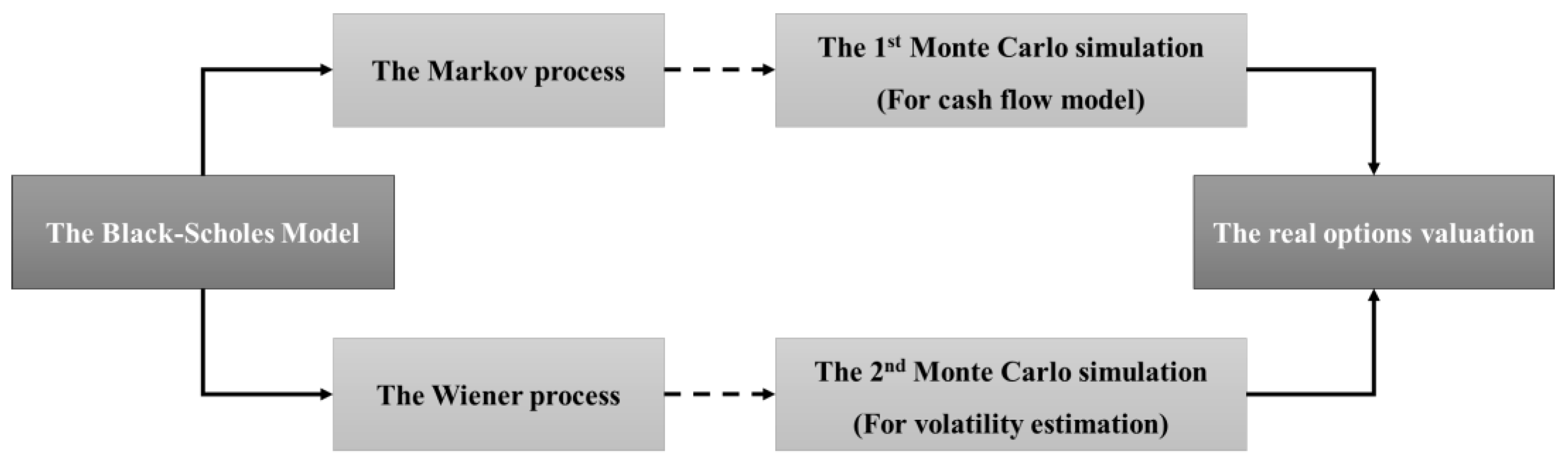
This study analyzes how ROV applies to projects. Applicability of the project to ROV requires two Monte Carlo simulations (MCSs) to satisfy a Markov process and a Wiener process [28]. First, this study proposes a cash flow model using a MCS to satisfy the Markov process in the project. A MCS is a method of iteratively extracting the PV of cash flows at random according to a probability distribution of input data, such as CAPEX, OPEX, and revenue. In practice, project cash flows change continuously over time. Thus, the overall project value can also change continuously. If the distribution of the rate of return on the PV of the cash flows from the second MCS is a standardized normal distribution with a mean of 0 and variance of 1, the Wiener process is also satisfied. Figure 1 illustrates a flow diagram of the conditions for satisfying applicability to a project from the Black-Scholes model to ROV.

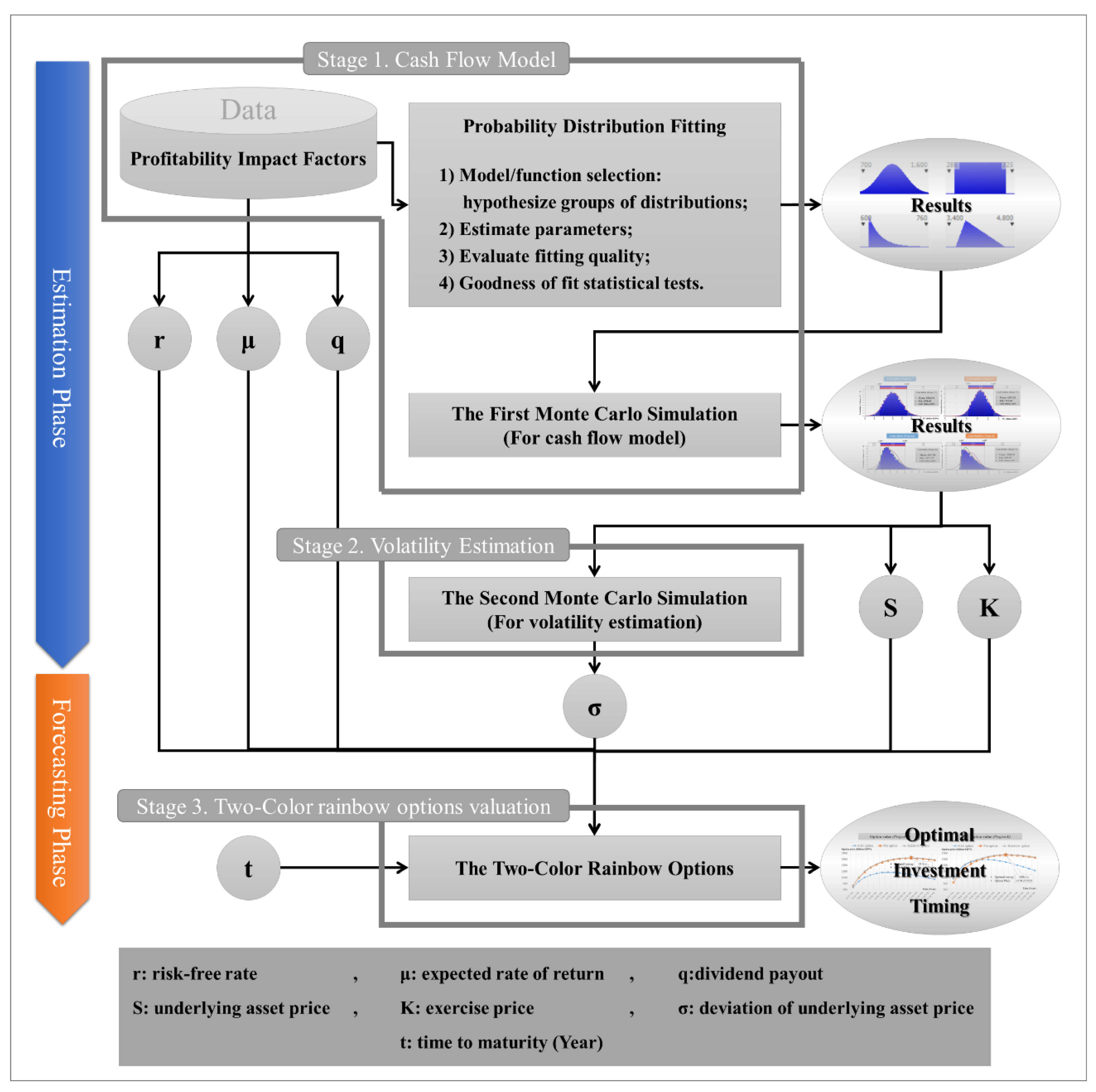
Projects occur in large, heavy industry, and thus require caution in making project investments due to the irreversibility of the investment. This section presents a framework for project investment decisions using ROV of two-color rainbow options, which considers the volatilities of cash inflow and outflow. Figure 2 illustrates the framework of ROV and can be divided into two phases: an estimation phase and a forecasting phase. The estimation phase determines the distribution of the underlying asset price through the historical data of CAPEX, OPEX, and revenue, which affect the ROV. The distribution derived from the estimation phase is used as an important parameter of the ROV. The forecasting phase predicts the project value by deriving the ROV by changing the time to maturity from one year to 20 years later. The forecasting value can be used to determine the optimal investment timing since it represents the project value at that time.

The following describes in detail each of the three stages shown in Figure 2.

3.1. Cash Flow Model

Projects can be used as real assets in an asset price determination through the cash flow model. Therefore, it is necessary to apply a cash flow model appropriate for the characteristics of the project. To construct a cash flow model, the first step is to define the profitability impact factors affecting the project value. This study presents three major factors from components of a pro forma income statement, which provides the following profitability impact factors: CAPEX, OPEX, and revenue.

The net present value (NPV) of the project can be calculated as the PV of cash inflow (revenue) minus the PV of cash outflow (CAPEX and OPEX) using the DCF method. However, the disadvantage of the DCF method is that it does not account for the volatility of profitability impact factors and, therefore, does not adequately reflect the risks in the future. To overcome the weakness of the DCF method, some studies proposed evaluating the value of the cash flow model considering the variability of profitability impact factors using MCS [29,30,31]. The probability distributions of profitability impact factors can be drawn by probability distribution fitting, which can help provide an accurate value forecast for the project. Probability distribution fitting is the fitting of a probability distribution over collected data with repeated measurements of statistical variables, and a procedure for selecting a statistical distribution best suited to a dataset [32]. The authors calculate the probability distribution fitting using the commercial statistical software, @Risk for Excel Version 6.3.1 (Palisade Corporation, Ithaca, NY, USA).

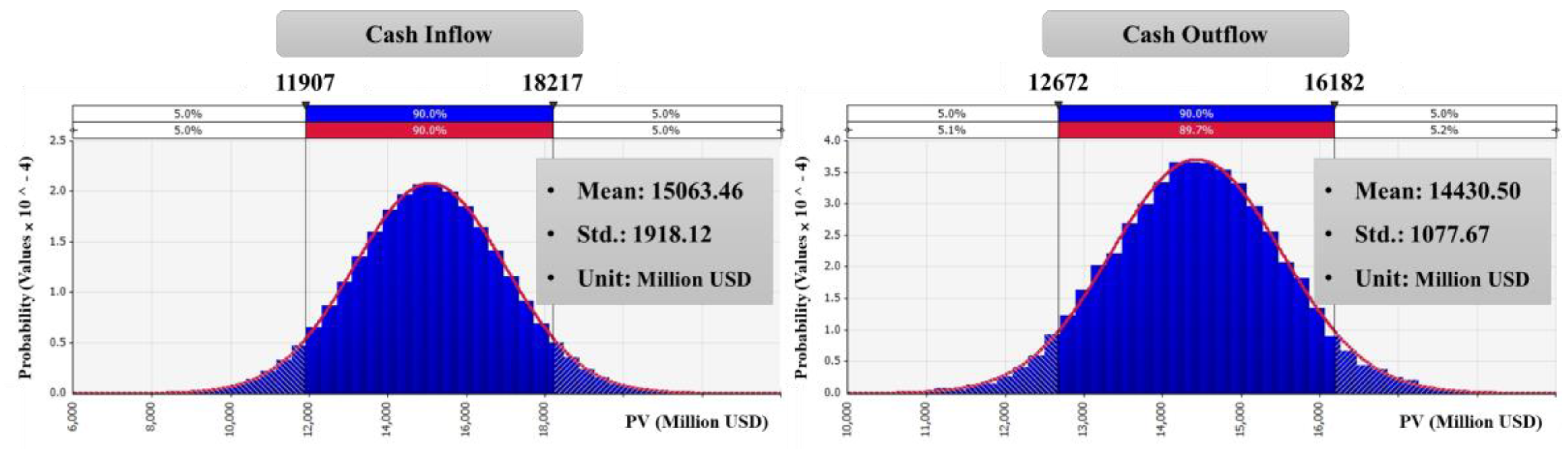
The MCS of the stochastic process extracts the random outputs of the stochastic process. The probability distribution is used as input data to account for the uncertainty of risks. Two MCSs are used to meet separate purposes. The first MCS provides the distribution of the underlying asset and the second MCS yields the volatility of the rate of return for the underlying asset as a variable required for the ROV. The input data for the first MCS is the probability distribution of the profitability impact factors, and the input data for the second MCS is the probability distribution of cash inflow and outflow, which also result from the first MCS.

Table 1. Summary of Monte Carlo simulations for the ROV (source: authors’ design, 2017).

Monte Carlo Simulation	Input Data	Output Data	Object
First MCS	Probability distributions of profitability impact factors	Probability distribution of the present values of cash inflow and outflow	Cash flow model (to satisfy Markov process)
Second MCS	Probability distribution of the present values of cash inflow and outflow	Probability distribution of the cash inflow and outflow converted into a standardized normal distribution	Volatility estimation (to satisfy Wiener process)

summarizes the process of the two MCSs.

3.2. Volatility Estimation

The purpose of the second MCS is to simulate the volatility of the rate of return on the underlying asset. This is obtained by converting the first MCS outputs to the PV and uses them as inputs for the second MCS. Using the probability distribution of the underlying asset from the first MCS, it is possible to transform the distribution of the rate of return for the underlying asset into a standardized normal distribution with a mean of 0 and a variance of 1 to satisfy the Wiener process. The formula for obtaining the converted PV is as follows:

$$P{V}_n=Std. \times \mathrm{rand}\left({\mathrm{x}}_n\right)+\mathrm{Mean}$$

(1)

where Std. is a value of the standard deviation from the probability distribution of the underlying asset, Mean is the value of the mean from the probability distribution of the underlying asset, rand(x_n) is a random variable generator of the standardized normal distribution, and n is the number of trials from the second MCS.

The rate of return can is expressed using Equation (2) [33]:

$$k_n=\ln \left(\frac{P{V}_{n + 1}}{P{V}_n}\right)$$

(2)

where k_n is the rate of return.

The result of the deviation for the rate of return is used as the volatility in the ROV.

3.3 .Two-Color Rainbow Options Valuation

The fundamental hypothesis of OPM is that the value of underlying assets should be greater than zero. If NPV of a project is taken as the underlying asset in the ROV, the hypothesis could not be satisfied because the underlying assets can have a zero, or negative, value. Therefore, various studies focused on the ROV with the volatility of cash inflow (revenue) from a project as the underlying asset [2,10,12,22,23,24,34,35,36,37,38]. Additionally, the volatility of both cash outflow and cash inflow is a critical factor affecting the value of the project. Thus, it is reasonable to use exotic options for a project, such as the rainbow option.

This study uses the rainbow option with n = 2, called two-color rainbow options valuation [27]. Rubinstein [39] stated that two-color rainbow options are options for two volatile assets that cannot be interpreted as options for only one underlying asset. They also categorized two-color rainbow options into 10 types. Among the 10 types of options, this study uses a dual-strike call/put type suitable for steel plant projects, so the equation at maturity is:

$$\max \left[\left(S_{in}-K_{in}\right),\left(K_{out}-S_{out}\right),0\right]$$

(3)

where S_in and S_out are the underlying assets for cash inflow and outflow, respectively, K_in and K_out are the exercise prices for cash inflow and outflow, respectively, S_in ≠ S_out, K_in ≠ K_out, max[(S_in − K_in), 0] means call options at maturity, and max[(K_out − S_out), 0] means put options at maturity.

European options are those that can only be stroked at maturity, and American options are those that can be stroked at any time within maturity. To apply OPM in ROV, it is necessary to consider the possibility of exercising the rights to defer before maturity. Therefore, ROV is likely to be an American option. European options need to approximate American options so that investors can exercise the right before maturity. This approximation is called Black’s approximation [40]. This method calculates the prices C_T and C_t of European options with maturity T and t (t < T) using OPM, where the price that satisfies the condition of max (C_T, C_t) determines the price of the American options.

Applying Black’s approximation, this study obtains an optimal invest timing value V_op with the following equation:

$$V_{op}=\max \left[\begin{array}{c}\left(S_{in,t}{e}^{-qt}\mathrm{N}\left(d_{in, 1}\right)-K_{in,t}{e}^{-rt}N\left(d_{in,2}\right)\right),\\ \left(K_{out,t}{e}^{-rt}N\left(-d_{out,2}\right)-S_{out,t}{e}^{-qt}N\left(-d_{out,1}\right)\right),\\ 0\end{array}\right]$$

(4)

where:

$$\begin{array}{l}{d}_{in,1}=\frac{\ln \left(\frac{S_{in,t}}{K_{in,t}}\right)+\left(r-q+\frac{1}{2}{\sigma }_{in}{}^2\right)t}{{\sigma }_{in}\sqrt{t}}, d_{in,2}=\frac{\ln \left(\frac{S_{in,t}}{K_{in,t}}\right)+\left(r-q-\frac{1}{2}{\sigma }_{in}{}^2\right)t}{{\sigma }_{in}\sqrt{t}}=d_{in,1}-\sigma \sqrt{t}\hfill \\ d_{out,1}=\frac{\ln \left(\frac{S_{out,t}}{K_{out,t}}\right)+\left(r-q+\frac{1}{2}{\sigma }_{out}{}^2\right)t}{{\sigma }_{out}\sqrt{t}}, d_{out,2}=\frac{\ln \left(\frac{S_{out,t}}{K_{out,t}}\right)+\left(r-q-\frac{1}{2}{\sigma }_{out}{}^2\right)t}{{\sigma }_{out}\sqrt{t}}=d_{out,1}-\sigma \sqrt{t}\hfill \end{array}$$

(t = 1, 2,·····, T, where t is a maturity of the option).

N(x) is a cumulative probability distribution function of x for a standardized normal distribution, S_in,t is PV of cash inflow as the underlying asset, K_in,t is PV of cash outflow as the exercise price, σ_in is a volatility of the rate of return on cash inflow, S_out,t is PV of cash outflow as the underlying asset, K_out,t is PV of cash inflow as the exercise price, σ_out is a volatility of the rate of return on cash outflow, r is a risk-free rate, and q is an opportunity cost for project delay (the dividend payout).

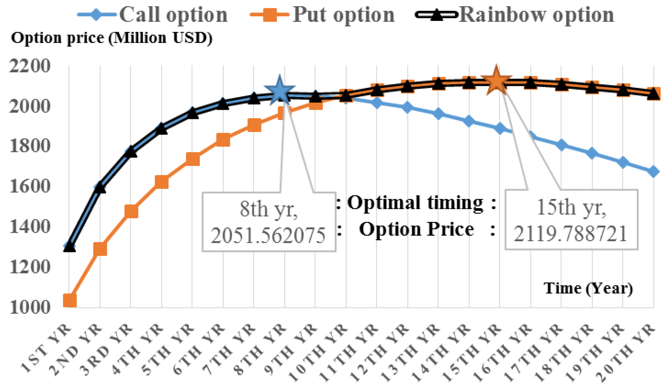
The value of options has a correlation of 1 with the value of the project. Therefore, investors can choose the time t from the highest option value as the optimal investment timing.

4. Case Study

4.1. Background

Steel plants are a component of an especially heavy industry and operate with a collection of high-cost equipment that affects CAPEX. OPEX is also quite high because plant reliability and automation are critical in a continuous process industry that operates 365 days per year. In addition, plant operations usually require revamps that involve replacing major equipment for each process every 15 to 20 years. The quality of steel products is not only heavily influenced by operational experience, but also the quality of materials, especially that of iron ore and coal. The price of steel products has a positive correlation with the price of materials (refer to Figure 3). As Figure 3 shows, the price volatility of raw materials and steel products has increased sharply since 2004. Therefore, to overcome these issues and make reliable investment decisions, investors must evaluate options to defer a steel plant project and to propose optimal investment timing.

4.2. Data Collection and Parameters of a Project

This study examines a case of cash flow for a steel plant project C (Brazil, 2011), which contains profitability impact factors assumed based on the data for the project at that time. In traditional DCF methods, all profitability impact factor values are fixed and each factor has only one value. However, if these values vary due to uncertain environments, each profitability impact factor can have a probability distribution, which provides input data to determine the probability distributions of the PVs of cash inflow and cash outflow using MCS. First, revenue, which is the profitability impact factor of the cash inflow, is obtained by multiplying the production by the unit price of the product. Production is assumed to be a constant value of 3 million tons, and the distribution of profitability impact factor is obtained through the annual volatility of the unit price of the product [41]. Second, the distributions of CAPEX and OPEX, which are profitability impact factors of cash outflow, are as follows: CAPEX reflects the cost growth in the PERT distribution based on cases of over 160 analyzed design build projects [42]. OPEX consists of raw material and other costs to produce the product. The distribution of profitability impact factor is obtained by reflecting the volatility of the raw material costs [41]. The source data are used as the input for the probability distribution fitting using the statistical program @Risk. The probability distribution fitting makes the probability distributions fit a set of data accumulated for 15 years (from 1996 to 2011) for the variable profitability impact factors.

Some of additional factors in

Table 2. Case information for the cash flow model.

Profitability Impact Factors	Unit	Project C (Brazil, 2011)			Source of Data (Using @Risk)
		Deterministic Model	Probability Model
		Fixed Value (for DCF)	Probability Distribution	Variation (for ROV)
CAPEX	Million USD/Project	3800	PERT	Min: 3800 Mode: 3882 Max: 3990
OPEX	Million USD/Year	813	Normal	Mean: 813 Std.: 130
Revenue	Million USD/Year	1920	Normal	Mean: 1920 Std.: 281
Additional factors (source of data: project plan documents) ◆ Construction Period/Business Period: 4 Years/20 Years ◆ Corporate tax rate: 34% ◆ Debt-to-Capital ratio: 0.5 (debt: 50%, Equity: 50%) ◆ Risk free rate: 3.691% ◆ Market risk premium: 7.219% ◆ Beta: 0.91 ◆ Cost of debt before tax: 4.311% ◆ WACC: 4.873% ◆ Country risk premium: 3.400% ◆ Discount rate: 8.273%

required to obtain the cash flow model are determined by calculation. The cost of capital according to the weighted average cost of capital (WACC) consists of the cost of equity (CoE), cost of debt before tax (CoD), debt-to-capital ratio (DC_ratio), and corporate tax rate (tax). In this case, the cost of equity is derived using the capital asset pricing model [20]. The model also includes the risk-free rate (r), market risk premium (R_m), and beta (β). The cost of debt refers to the borrowing interest rate in project financing:

CoE = r + β × (R_m − r)

(5)

WACC = (1 − DC_ratio) × CoE + DC_ratio × CoD × (1 − tax)

(6)

To calculate the project’s profitability, it is essential to obtain a discount rate (μ), which is an index of project risks:

μ = WACC + Country risk premium

(7)

4.3. Results

The case study makes several assumptions. In Table 2, the order of CAPEX spending goes from equity to debt. Loan repayment is a method of fully amortizing a loan and starts after five years from the beginning of a business period. Principal repayment is evenly repaid during the remaining business period. This study assumes that all CAPEX is a depreciable asset and is amortized on a straight-line basis. All output is sold every year, so there is no inventory of goods. Net working capital is the cost to operate the plant and is spent one year ahead of the business period and recovered in the last year of the business period.

Project cash flow is divided into the construction period and business period, each of which constitutes the cash inflow and outflow associated with the three profitability impact factors presented in Table 2 and

Table 3. Cash flow data sheet for Project C (2011, Unit: million USD).

Period	Construction (4 Years)				Business (20 Years)
Year	1	2	3	4	5	···	21	22	23	24
Cash outflow	(950)	(950)	(991)	(1152)	(1369)	···	(1413)	(1409)	(1406)	(1282)
CAPEX	(950)	(950)	(950)	(950)	-	···	-	-	-	-
OPEX	-	-	-	(120)	(1003)		(1003)	(1003)	(1003)	(983)
Financial cost	-	-	(41)	(82)	(82)	···	(149)	(143)	(138)	(132)
Tax	-	-	-	-	(284)	···	(261)	(263)	(265)	(267)
Cash Inflow	-	-	-	-	1985	···	1985	1985	1985	1985
Revenue	-	-	-	-	1920	···	1920	1920	1920	1920
Depreciation saving	-	-	-	-	65	···	65	65	65	65
Net cash flow	(950)	(950)	(991)	(1,152)	616	···	572	575	579	703

. This study calculates project profitability with a deterministic NPV.

$$\mathrm{NPV}= {{\displaystyle \sum }}_{t=1}^N\frac{R_t}{{\left(1+\mu \right)}^{t-1}}, \mathrm{so} \mathrm{the} \mathrm{deterministic} \mathrm{NPV} =823.34 \mathrm{Million} \mathrm{USD}$$

(8)

where t is the project period, N is the total project period, R_t is annual cash flow, and μ is the discount rate.

Apart from the deterministic NPV model, this study can build a cash flow model as a probabilistic NPV model that reflects the volatility of profitability impact factors. The authors show the first MCS using the probability distributions of the profitability impact factors for the case in Table 2. The number of simulation repetitions is set to 10,000 to ensure a dependable simulation. The left side of Figure 4 shows the probability distribution for the PV of cash inflow and the right side shows that of cash outflow. The figures also show the means and standard deviations, as well as the upper and lower 5% values according to the probability distribution fitting.

From these distributions, it is possible to obtain a probabilistic NPV assuming that the mean value is a representative value for these distributions. Therefore, the probabilistic NPV of Project C is $632.96 (15,063.46 − 14,430.50) million USD. If investors do not have a specific investment strategy, the investment can be approved by a DCF criteria that NPV of the project is greater than zero. However, the probabilistic NPV can vary depending on the PVs of cash inflows and cash outflows. The deterministic NPV ($823.34 million USD) is also one of the probabilistic NPVs. However, in the extreme cases of probabilistic NPVs in Figure 4, if the cash inflow has a value below 5% ($11,907 million USD) and the cash outflow has a value above 5% ($16,182 million USD), the NPV of the project will be negative ($−4275 million USD) and the investment must be rejected. To prepare for these uncertainties, it is critical to determine the optimal investment timing that maximizes the project value.

The second Monte Carlo simulation is performed to estimate the volatility of rate of return of the project’s PVs for cash inflow and outflow. Substituting the mean and standard deviation values from the distribution of cash inflow and outflow of Project C into Equation (1), the authors arrive at the results in

Table 4. PV of cash flow for a steel plant project.

Case	PV of Cash Inflow	PV of Cash Outflow
Project C	PVin,n = 1918.12 × rand(xin,n) + 15,063.46	PVout,n = 1077.67 × rand(xout,n) + 14,430.50

.

Equation (2) is used to perform the second Monte Carlo simulation 10,000 times to determine the volatility of the rate of return on the project’s PVs for cash inflow and outflow. The results are shown in

Table 5. Volatility of the rate of return of a steel plant project’s PV.

Case	Volatility Estimation for Cash Inflow	Volatility Estimation for Cash Outflow
Project C	18.61%	10.68%

.

The results in Table 5 are used as the volatility for the ROV. All elements to apply ROV have been collected, and

Table 6. Elements to calculate the steel plant project’s ROV.

Notation	Description	Project C (Brazil, 2011)
Sin,t	PV of cash inflow as the underlying asset	$15,063.46 million USD
Kin,t	PV of cash outflow as the exercise price	$14,430.50 million USD
σin	volatility of the rate of return on cash inflow	18.61%
Sout,t	PV of cash outflow as the underlying asset	$14,430.50 million USD
Kout,t	PV of cash inflow as the exercise price	$15,063.46 million USD
σout	Volatility of the rate of return on cash outflow	10.68%
r	Risk-free rate	3.691%
μ	Discount rate	8.273%
q	Notion of opportunity cost for project delay	4.582%

summarizes the elements.

The elements S_in,t, K_in,t, S_out,t, and K_out,t were derived from the first MCS, and the elements σin and σout were derived from the second MCS. Otherwise, r is the risk-free rate as the mean London Inter-Bank Offered Rate for the past 15 years, μ is a discount rate based on the capital asset pricing model; and q is the opportunity cost of the project derived from the market price of risk calculated as μ − r [19].

Substituting the elements in Table 6 for each project and the maturity of the option, t, from one year to 20 years into Equation (4) yields the results illustrated in Figure 5. To illustrate the optimal investment timing, the time (year) is on the horizontal axis and the option price (million USD) is on the vertical axis. In the legend of Figure 5, the call option is the option price when cash inflow is the underlying asset, and the put option is the option price when cash outflow is the underlying asset. Finally, the rainbow option indicates the price of the two-color rainbow options when it is the underlying asset, considering both cash inflow and cash outflow. In Figure 5, the orange star shows the optimal investment timing and option value derived from the rainbow option, while the blue star shows the optimal investment timing and option value derived from the call option, which is the conventional method.

5. Discussion

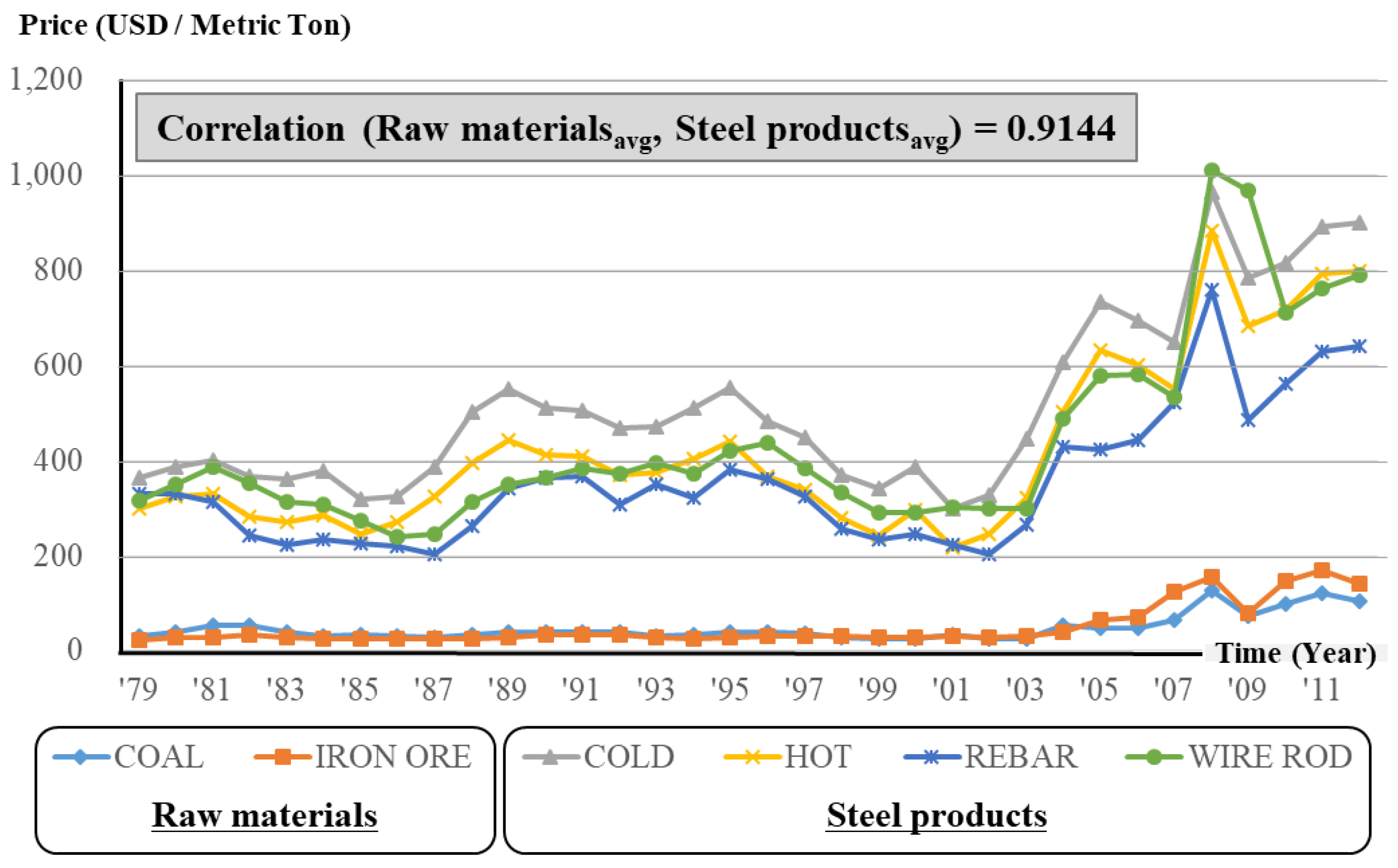
In order to maintain sustainable entrepreneurship in an unstable market, enterprises should develop steadily [43]. For the development of the enterprise, investors need to focus on long-term growth rather than short-term vision [44,45,46]. This study suggests the two-color rainbow option, which is a more robust model of real options valuation, to respond to the long-term unstable market for investors. The conventional method, real options valuation, focused on cash inflow volatility when evaluating the project value as call options. However, the proposed method, the two-color rainbow option, considers cash inflow and cash outflow simultaneously when evaluating project value as call options and put options. The inward cash flow volatility is associated with revenue volatility, and the product selling price is a major sub-factor of revenue. Outward cash flow volatility is associated with CAPEX and OPEX volatility, construction cost is a major sub-factor of CAPEX, and raw material price is a major sub-factor of OPEX. Based on the case study results, this paper suggests that it is more reasonable to consider both cash inflow and cash outflow when the correlation between raw material average price and product unit average price is 0.9144 (refer to Figure 3), as in the steel plant project. Steel plant companies typically link steel product prices to raw material prices to reduce risk. Therefore, the correlation between raw materials and steel products is close to 1. This result is similar in steel industries as well as oil and gas industries, power generation industries, and so on. Thus, these industries need to consider the volatility of cash outflow more than the volatility of cash inflow.

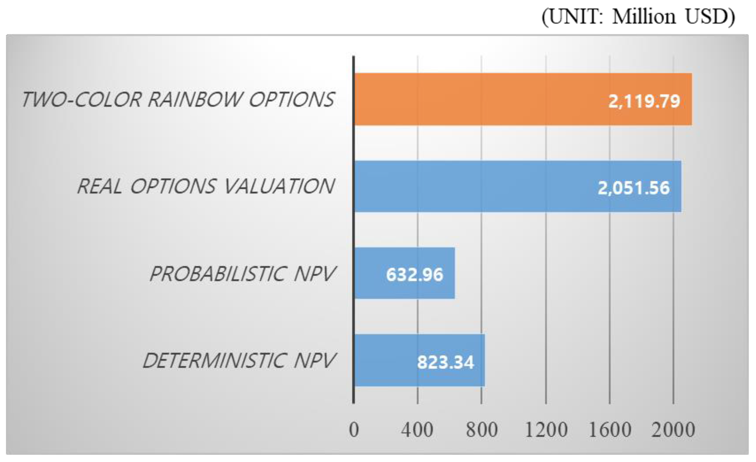
The above case study of the steel plant project effectively demonstrates the difference between the conventional method (real options valuation) and the proposed method (two-color rainbow options). The rainbow option result (15 years, $2199.79 million USD) differs from those for the call option (eight years, $2051.56 million USD) that earlier studies used to gauge optimal investment timing. The steel plant project case study is dominated by the put option by means of cash outflow, as well as the call option by means of cash inflow when determining optimal timing. Therefore, the authors suggest that investors should consider the volatility in both cash inflows and cash outflows in an investment decision based on the implied option value and NPV. Even if investors make an investment decision using only the DCF method, the investment can be approved without deferring the project since the NPV is greater than zero. However, investors who want to maximize profits can benefit more from making decisions based on the method proposed in this study. In economics, rational investors demand compensation for risk, so the price of an asset necessarily reflects the magnitude of the risk that the asset has [20]. Thus, rational investors in this paper will choose the option to make the best return, if the project is fully reflected in risks. The results are summarized in Figure 6 below.

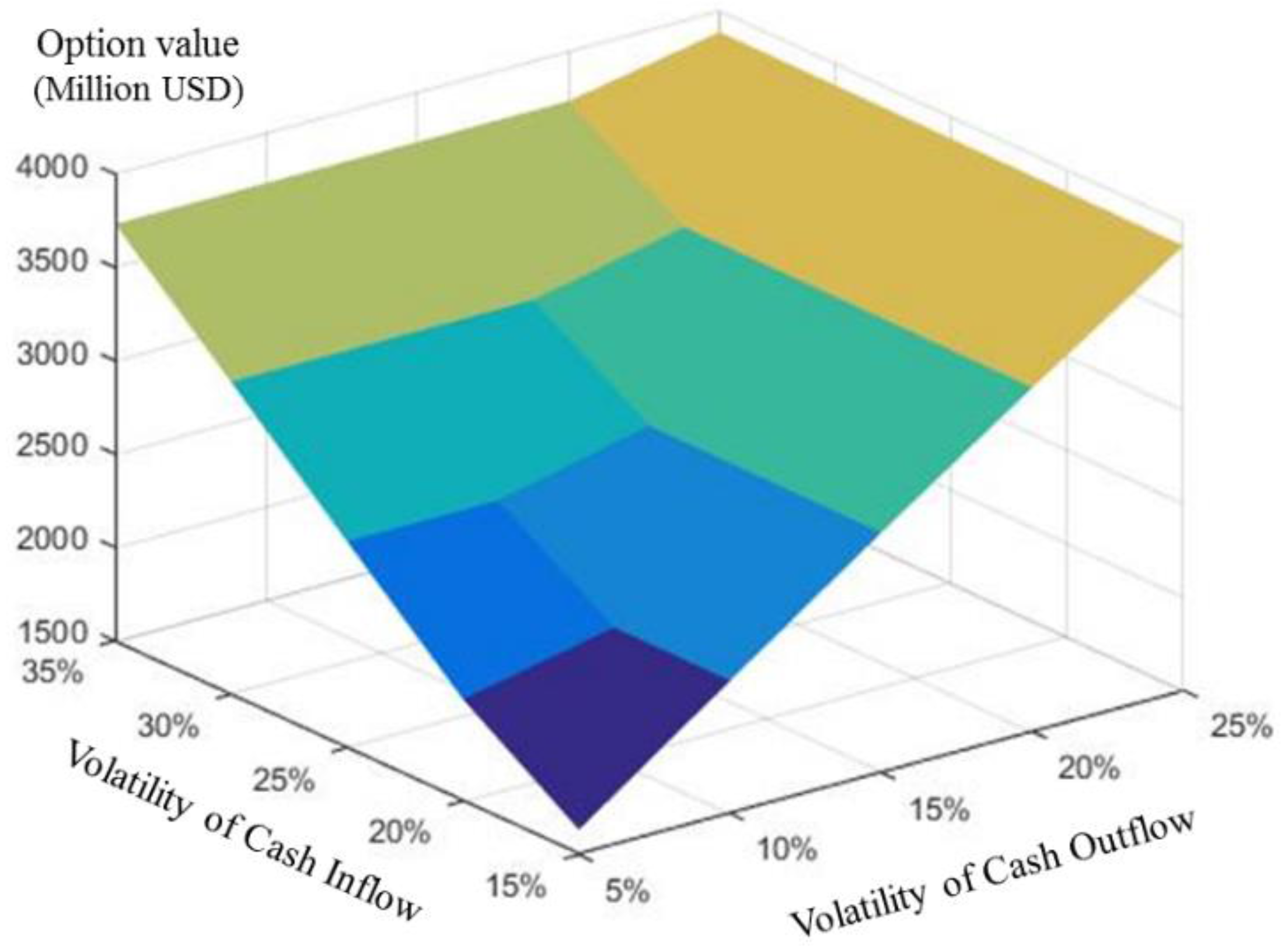
This paper additionally confirms the conditions under which the proposed two-color rainbow options and existing real options valuations yield the same results. The parameters σ_in and σ_out affect the option value, where σ_in represents the volatility of the rate of return on cash inflow, and σ_out represents that for cash outflow. In this study, the sensitivity analysis of σ_in and σ_out is conducted to check the change of the options value as the volatility of the underlying asset changes.

Table 7. Sensitivity analysis for the optimal investment condition.

		Volatility of Cash Inflow
		15%		20%		25%		30%		35%
Volatility of cash outflow	5%	8th year	1633	9th year	2212	9th year	2785	9th year	3343	9th year	3882
		Call		Call		Call		Call		Call
	10%	15th year	2046	9th year	2212	9th year	2785	9th year	3343	9th year	3882
		Put		Call		Call		Call		Call
	15%	14th year	2605	14th year	2605	9th year	2785	9th year	3343	9th year	3882
		Put		Put		Call		Call		Call
	20%	13th year	3173	13th year	3173	13th year	3173	9th year	3343	9th year	3882
		Put		Put		Put		Call		Call
	25%	13th year	3732	13th year	3732	13th year	3732	13th year	3732	9th year	3882
		Put		Put		Put		Put		Call
		A	B	A is optimal investment timing (Year), B is option value (Million USD),
		C		and C is option type dominated by the Two-color rainbow options

Note: An asymmetric relationship with cash inflow and cash outflow is expressed in color. Blue region is dominated by the cash inflow and is affected by the call option. Red region is dominated by the cash outflow and is affected by the put option.

shows the sensitivity analysis for σ_in and σ_out.

Table 7 and Figure 7 show that option value has an asymmetric relationship with both cash outflow and cash inflow. The two-color rainbow options consist of two option values: the call option (volatility of cash inflow) and put option (volatility of cash outflow). Basically, the greater the volatilities of cash inflow and outflow, the greater the option value is. Since volatility is in proportion to the risk, it means that the values of risks increase. As the volatilities increase, the optimal investment timing increases, and the put option has a greater optimal investment timing than the call option. In Table 7, the call option has a condition governing the value of the rainbow option: the volatility of cash inflow should be about 10% greater than that of cash outflow. In finance, call options generally have favorable trading conditions compared to put options. In this case, the Black-Scholes model without dividends is applied. The Black-Scholes model applied in this paper is based on opportunity cost instead of dividends. Therefore, ROV is represented by the asymmetry of the volatility effect. The intuitive analysis, not technical analysis, is as follows: a problem that needs to consider the order of cause and effect; Cause: prices of iron ore and coal rose or fell. Effect: steel prices go up or down. This logic, created by the practices of the steel plant project, explains that the cash outflow affects the cash inflow through the phenomenon that the led cause affects the lagged result. Therefore, this can be seen that put options occurs as a more important factor than the call options do because put options occur as a led cause in the steel plant project. In the case study of steel plant project, the two-color rainbow option evaluation model proposed in this paper can provide more effective results to investors when the difference between inward cash flow volatility and outward cash flow volatility is not large. This means that the two-color rainbow option evaluation model can help investors achieve sustainable entrepreneurship with rational decision-making. Therefore, this study confirms the necessity to consider the volatility of cash outflow during the project planning stage through the sensitivity analysis.

6. Conclusion and Future Work

For economic sustainability, investment decisions require due consideration of the features of steel plant projects, which are irreversible. Although traditional discounted cash flow methods are conveniently implemented using datasheets, they cannot account for the volatility of the risk factors that affect the value of projects. Therefore, an approach to support decision-making that can be easily integrated into the discounted cash flow method, and that reflect these risks of projects, is needed. This study analyzed a steel plant project and showed that the volatilities in the present value of the project cash outflow and inflow are decisive factors in the project value, unlike models presented in previous studies. To apply these factors, unlike regular real options valuation, this study applied real options valuation to the exotic two-color rainbow options. Effectively, this study confirmed that the value of options was dominated by the volatility in the present value of cash outflows rather than that for cash inflows through a case study. By altering the two factors of uncertainty, the sensitivity analysis provides significant insights for optimal investment timing and clarified the dominant factor for a type of option. This study contributes a finding that suggests that investors prioritize cash outflow when investing in projects for sustainable development. If projects are to support decision-making on ROV, such as a refinery plant, power plant, aviation industry, automobile industry, and semiconductor industry, where the project is considered both seller and buyer positions, the authors suggest using the two-color rainbow options model.

However, this study has two limitations. First, the Black-Scholes model considers only the volatility of the underlying asset and does not consider the volatility of the exercise price. To overcome this matter, this study proposed incorporating the volatilities of cash inflow and cash outflow as different types of options based on an exotic option valuation. However, the proposed option model does not account for the correlation of the two factors, so it is possible that the results may be less realistic. Therefore, it is necessary to present a model besides the Black-Scholes model in a future study. Second, this study considered multiple profitability impact factors in the cash flow model, but assumed that the cash flow model is constructed independently in each profitability impact factor because the study performed the first Monte Carlo simulation based on each profitability impact factor without a relationship among profitability impact factors. Future proposals can offer more accurate and reasonable estimations of cash flow using statistical theories or data mining methods to determine the correlation among each profitability impact factor. Recent advances in artificial intelligence technology can help investors make decisions through economic sustainability assessment using more accurate forecasting techniques to replace traditional methods, such as Monte Carlo simulation. Fuzzy theory, artificial neural networks, and machine learning will help researchers develop methodologies to generate more accurate predictions and reasonable investment decision methodologies.