Abstract
Infrastructure not only plays an import role in socioeconomic development, but also results in a remarkable increase of CO2 emissions. Based on a panel data analysis of 29 provinces in China from 1995 to 2013, we investigated the relationship between socioeconomic development and CO2 emissions with special focus on the impact of infrastructure stock density in both the country and regional scales. The results confirmed that a 1% increase of material stocks in infrastructure per built-up area would lead to a 0.11% decrease in CO2 emissions at the country level. The effect of infrastructure stock density on CO2 emissions varied across regions, for which elasticity was −0.34, 0.06, and 0.14 for the eastern, central, and western region, respectively. In order to achieve a low-carbon and sustainable development, it is crucial to improve the spatial compactness of infrastructure in the future. Policy implications include upgrading the economic structure to a low-carbon one for the eastern region, accelerating the development of renewable energy infrastructure, and constructing and utilizing infrastructure in an energy-efficient way for the central and western regions.
1. Introduction
Infrastructure development is one of the most important consequences of urbanization. On one hand, it provides fundamental functions and services to the society so as to meet humans’ needs for housing, transportation, water supply, and so on, which secures societal wellbeing and in return supports further urbanization. On the other hand, the development of infrastructure is also a process of material metabolism, which includes a huge amount of materials flowing into, stocking in, and flowing out of the built environment. Each life stage of infrastructure (i.e., resource extraction, material production, construction, operation, demolition, and waste management) involves a large consumption of energy, and thus results in a sharp increase of CO2 emissions [1,2]. Taking the building sector as an example, it accounted for 32% of global energy use and generated 9.18 Gt CO2 emissions in 2010 [3]. Moreover, because of the decades- or even century-long lifetime of infrastructure, it may increase the risk of locking the society into an energy-intensive and high-emission path, which is usually costly and hard to change [4].
As the world is continuously becoming urbanized, over 70% of population will live in cities by 2050 [5], which implies that more infrastructure needs to be constructed. Meanwhile, the restriction of global mean temperature rise below the 2-degree threshold also poses great challenges to our future development [6]. Due to the important and enduring roles of infrastructure in shaping the socio-economic and climate change paths, it is necessary and fundamental to reveal the correlation between infrastructure and CO2 emissions, so that effective policies could be designed to direct the infrastructure development toward a low-carbon and sustainable way.
In the past decades, the great changes in socio-economy driven by urbanization and their impacts on CO2 emissions have been widely discussed. A variety of factors have been found to have significant impacts on CO2 emissions, such as urbanization level, economic development, urban population density, and urban forms. For example, Poumanyvong and Kaneko [7] suggested that the impact of urbanization on CO2 emissions was positive for all income groups, while Sharma et al. [8] held the opposite opinion that urbanization has a negative and statistically significant impact on CO2 emissions for the global panel. Fang et al. [9] selected a series of urban form indicators and found that increased urban continuity will led to reductions in CO2 emissions and that, conversely, increased urban shape complexity and exerted a positive influence in relation to CO2 emissions. Yang et al. [10] found that socio-economic development and increased income were the primary driving factors for the growth of per capita CO2 emissions from transportation. Besides this, some studies have indicated the giant emissions caused by buildings and transport infrastructure and their great potential in emission mitigation. For example, Liu et al. [11] estimated the on-road energy use and CO2 emissions in China from 1978 to 2008. Muller et al. [2] calculated the embodied carbon emissions of existing infrastructure stocks at global scale in 2008. Although a recent study has affirmed the effect of cement, aluminum, and steel stocks of global build environment on CO2 emissions [12], most of the previous studies mainly focused on the accounting of material stocks, their related carbon emissions, and the capacity for climate change mitigation in the future [13,14]. The impact of infrastructure stocks on CO2 emissions especially in developing economies is still not well understood.
China, as the most rapidly urbanizing country in the world during the last three decades [15], has witnessed an unprecedented development of its infrastructure, both in scale and in speed. During the last decade, the floor space of buildings soared at an annual rate of 17.9% from 1995 to 2015, while the length of railway and road increased by 0.9 and 2.9 times, from 0.06 to 0.12 kilometers and 1.16 million kilometers to 4.58 million kilometers, respectively [16]. Accordingly, a massive consumption of construction materials (especially those with high environmental footprint, such as steel, cement, and lime) and energy has put China under astonishing environmental pressures. For example, cement consumption in China reached 2160 million tons in 2012, accounting for 58% of the world total [17]. Meanwhile, China has become the largest carbon emitter in the world since 2006, and was responsible for approximately 37% of global committed emissions from existing energy and transportation infrastructure [18]. In addition, China is a country with significant regional disparity, whose socioeconomic conditions and distribution of infrastructure stocks among regions are both unbalanced [13]. Owing to the dramatic development of socio-economy and infrastructure, significant role in climate change, and distinct regional difference, China is an ideal case for expanding our knowledge on the effect of infrastructure stocks on CO2 emissions.
Through a panel analysis of 29 provinces in China from 1995 to 2013, we aim to investigate the relationship between socioeconomic development and CO2 emissions, and further discuss the impact of material stocks of infrastructure in both country and regional scales. Basically, we would like to address the following two research questions through China’s case study:
- (i)
- Does the accumulation of materials in infrastructure have a significant impact on CO2 emissions? What is the extent of the impact comparing to other socioeconomic factors?
- (ii)
- Will the impact vary across different levels of development and regions?
2. Materials and Methods
2.1. Material Stocks of Infrastructure and CO2 Emissions
As a premise to reveal the driving factors of CO2 emissions and to discuss the effect of infrastructure stocks on emission, the time-series data of CO2 emissions and material stocks (MS) of infrastructure at provincial level are needed.
Firstly, we adopted the standard Intergovernmental Panel on Climate Change (IPCC) guideline and local carbon emission coefficient to calculate China’s provincial CO2 emissions from fossil fuel consumption [19]. The detailed accounting method and emission factors can be found in Han et al. [20]. The statistics on energy consumption for 29 provinces during 1995–2013 were compiled from the China Energy Statistical Yearbook [21].
Secondly, material stocks were used as a proxy for infrastructure stocks, since it reflects not only the level of infrastructure development but also the quantity of material accumulation that has long-term effects on CO2 emissions [22,23,24]. In this study, a total of 13 types of infrastructure, including residential buildings, non-residential buildings, highways, roads (Class 1 to 4), railways (wooden sleeper and concrete sleeper), tap-water pipelines, sewerage pipelines, and gas pipelines, were considered for analysis due to their large share in total infrastructure and data availability. Ten types of major construction materials were accounted, including cement, iron, lime, brick, sand and gravel, glass, wood, plastic, asphalt, and ceramic. A bottom-up material flow analysis model was employed for material stocks estimation. The details on model description, parameter settings, and data sources can be found in our previous studies [10,25].
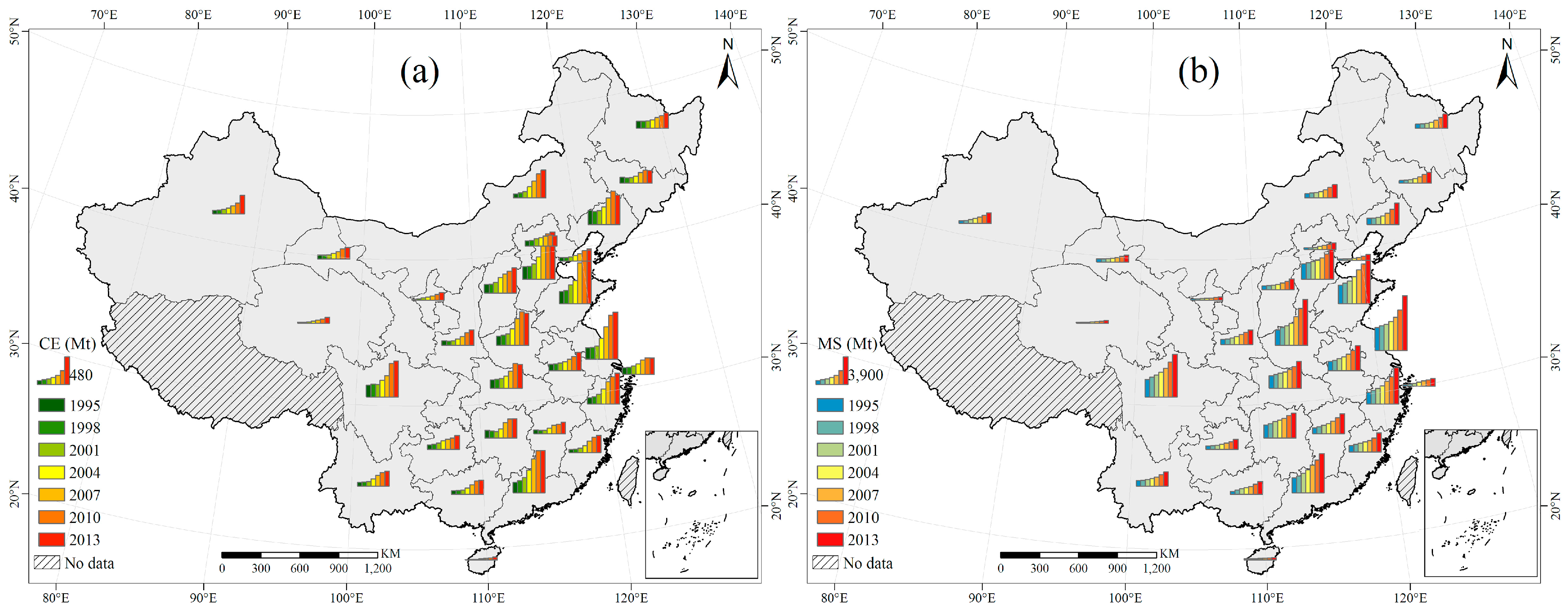
Figure 1 illustrates the estimated CO2 emissions and material stocks in infrastructure between 1995 and 2013. Similar temporal and spatial variations in CO2 emissions (Figure 1a) and material stocks (Figure 1b) can be found, which indicates an obvious correlation visually.
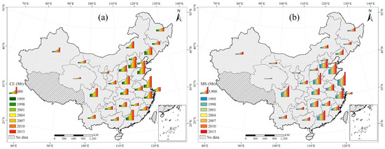
Figure 1.
Patterns of (a) CO2 emissions (CE) and (b) material stocks (MS) in China provinces, 1995–2013. Data are from our own estimation. Mt = Million tons.
2.2. A STIRPAT Model for Correlation Analysis
The IPAT identity, proposed by Ehrlich and Holdren [26], is a simple but useful conceptual model to decompose the driving factors of environmental impact (I) into three major aspects, that is population (P), per capita affluence (A), and technology (T). However, the simple assumption of each factor’s elasticity in a unitary value makes this identity unable to be used directly to test the impact of driving factors on environment [27]. For example, the Environmental Kuznets Curve (EKC) hypothesis assumed there is an inverted-U-shape relationship between income and environment, which cannot be explained by the IPAT identity. To address this limitation, the STIRPAT model was proposed as follows [28].
where, represents constant; b, c, and d are the coefficient of P, A, and T respectively; is the random error term; i is the unit of analysis.
After taking natural logarithms of both sides so as to minimize the heteroscedasticity, and considering several variables that may have impacts on CO2 emissions [29], Equation (1) is transformed as follows to facilitate a panel data analysis.
where, the subscripts i and t represents province and year respectively. is the coefficient of each variable. A means per capita GDP. The quadratic term of A was also introduced to check the EKC hypothesis. EI is energy intensity, measured as energy consumption divided by GDP. The higher value it has, the lower energy efficiency will be. U is the urbanization level measured by the share of urban population of the total. IND is the share of industry sector in GDP. Furthermore, the density of material stocks in infrastructure (MSD), expressed as MS divided by built-up area, was introduced to discuss the effect of infrastructure on CO2 emissions. Instead of the total amount, MSD is used as it enables the regional comparison. represents the unobserved region-specific effects (for example, geographic location, local climate, and fossil fuels endowments). is the within-entity error.
As pointed by Granger and Newbold [30], in order to conduct the panel regression analysis, the following two pre-tests will be needed: First is to check whether the time-series data are stationary or not. If it is stationary at its original value, it can be directly used for panel analysis. Otherwise, it must be tested through the following step. Second is to check whether two non-stationary time-series data have long-term common stochastic trends after the first-order differencing. If they do not have long-term common stochastic trends, it suggests that there exists cointegration between these two data sets and they can be used for panel regression. Otherwise their regression might be biased and inconsistent with the reality (i.e., the phenomenon of spurious regression).
Firstly, panel unit root test was used to measure the fluctuation characteristic of variables so as to avoid spurious regression. The null hypothesis of all the above four tests is that there exists unit root (i.e., the variables are non-stationary) among the cross sections (cross-sections mean different provinces in this study). The alternative hypothesis however is a little bit different from that in the LLC test, which assumes no unit root in the series (i.e., the variables are stationary). The other three tests allow unit root exists in some, but not in total cross-sections. Specifically, the LLC test was used to test the existence of homogeneity unit root while the other three were used to detect the heterogeneity unit root. Secondly, a panel cointegration test was employed to test whether there is a long-term relationship between the variables. Though there are many approaches for inspection, such as the Kao test, Larsson test, and Pedroni test, the Pedroni test was employed for the panel cointegration test due to its better performance than the Kao test and Larsson test when the time period is longer than 10 [31,32]. The null hypothesis of the Pedroni test is that there exists no cointegration between the variables.
In addition, the province-specific effect (i.e., in Equation (2)) should be evaluated as fixed effect or random effect to select the appropriate estimation method of panel regression models. Fixed effect assumes that the province effect is related to the explanatory variables while the Least Square Dummy Variable (LSDV) can be used for estimation. By contrast, random effect assumes the province effect is independent of all explanatory variables and Generalized Least Squares (GLS) is more effective to estimate the model. The Hausman test and Likelihood ratio test, two commonly used methods to confirm the effect [33], were subsequently applied.
Provincial data on P, A, U, IND, and EI were collected from the China Statistical Yearbook (1996–2014). GDP was converted into constant 1995 price in order to eliminate the effect of inflation or deflation. Built-up area data used for calculating MSD were mainly from the China Land and Resources Statistical Yearbook (1999–2004, 2010–2014), China Statistical Yearbook (2005–2009), and National land use change survey [34,35], in which missing data of some provinces in 1995 was complemented through linear interpolation. Table 1 provides a detailed description of variables used in this study. Tibet is excluded due to the lack of statistical data. To keep the data consistency, Chongqing is still regarded as a part of Sichuan province, since it was designated as a municipality in 1997.

Table 1.
Description of variables used for analysis.
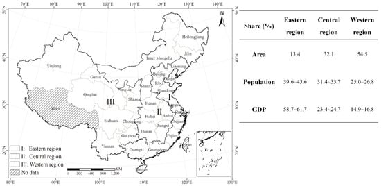
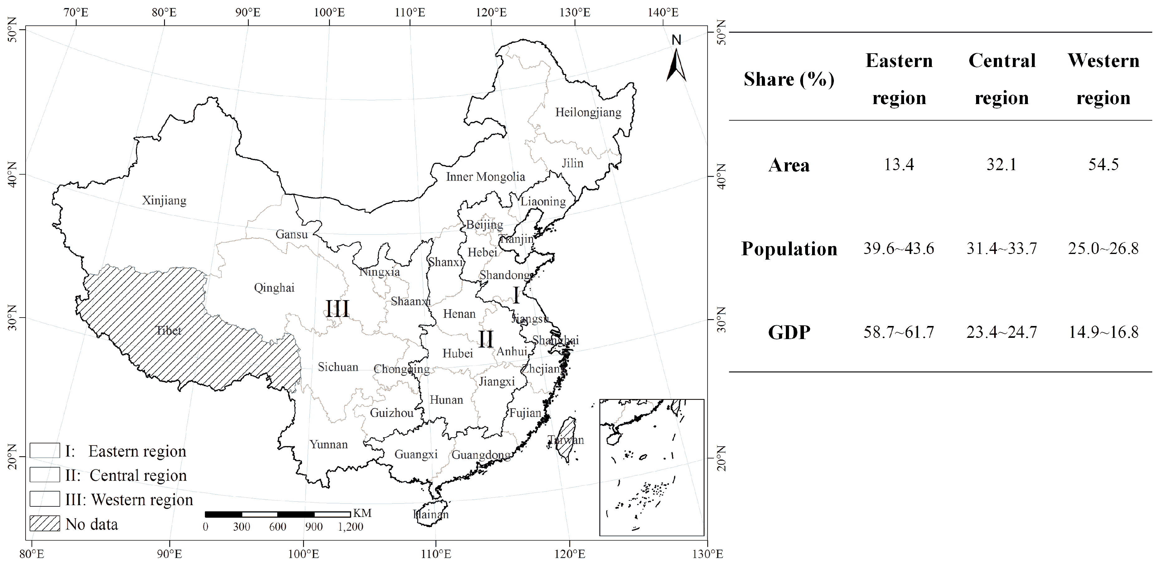
Figure 2.
Division and characteristics of three regions in China. Note: Since Chongqing was separated from Sichuan province and appointed as a municipality in 1996, it was still treated as a part of Sichuan province in the central region so as to keep the consistency. Tibet is excluded due to the lack of statistical data.
3. Results and Discussion
3.1. Panel Unit Root Test, Cointegration Test and Model Selection
Table 2 shows the results of panel unit root tests. All variables except population and urbanization are non-stationary in their level form, but they are all significantly stationary after first-order differencing. The results indicated that a cointegration test was necessary before building panel regression models.

Table 2.
Panel unit root tests.
Table 3 shows the results of the Pedroni residual cointegration test, which is composed of four statistics to test the cointegration within-dimension and three statistics to test the cointegration between dimensions. As shown in Table 4, the results of Panel v-Statistic, Panel rho-Statistic, and Group rho-Statistic accept the null hypothesis of no cointegration, but the results of Panel PP-Statistic, Panel ADF-Statistic, Group PP-Statistic, and Group ADF-Statistic reject the null hypothesis. Because of the higher power of PP-Statistic and ADP-Statistic than rho-Statistic when the time period is longer than 20 [36] and more rejections of null hypothesis, the results indicate that there exist long-run equilibrium relationships among the seven variables both at the national and regional levels, and regression models could be built.

Table 3.
Pedroni residual cointegration test.

Table 4.
Selection of panel regression models.
As reported in Table 4, all the results of Likelihood tests were significant at the 1% level, indicating that the fixed-effect models are preferred compared to the pooled regressions. The results of the Hausman test rejected the null hypothesis of random-effects models at the 1% significance level. In summary, the results suggested that the fixed-effect models and LSDV estimation method should be chosen for panel data analysis in this study.
3.2. Panel Regression Results in National and Regional Scales
Table 5 reports the effects of population, affluence, energy intensity, stock density, and other factors on CO2 emissions for the whole of China and three sub-regions respectively. At country level, coefficients for all factors except urbanization are statistically significant at the 1% level. The elasticity of CO2 emissions to population is 1.49, indicating that a 1% increase in population will lead to a 1.49% growth in CO2 emissions if other variables remain unchanged. The coefficient of GDP per capita is 1.33, which indicates that economic development also had a significant impact on emissions. In addition, the negative elasticity of the quadratic GDP per capita indicated the EKC relationship between economy and CO2 emissions in China. Energy intensity is another important factor affecting emissions, with an elasticity of 0.86. As for the effect of economic structure, a 1% increase in the share of the industrial sector in GDP would raise CO2 emissions by 0.21%. Notably, the negative but significant coefficient of material stock density could help to answer the first research question raised at the beginning of this study. It is confirmed that infrastructure stocks do have impacts on CO2 emissions, though its influence was smaller than other socioeconomic factors. However, when the spatial density of infrastructure stocks increase, CO2 emissions decline accordingly.

Table 5.
Panel estimation for the nation and the three sub-regions.
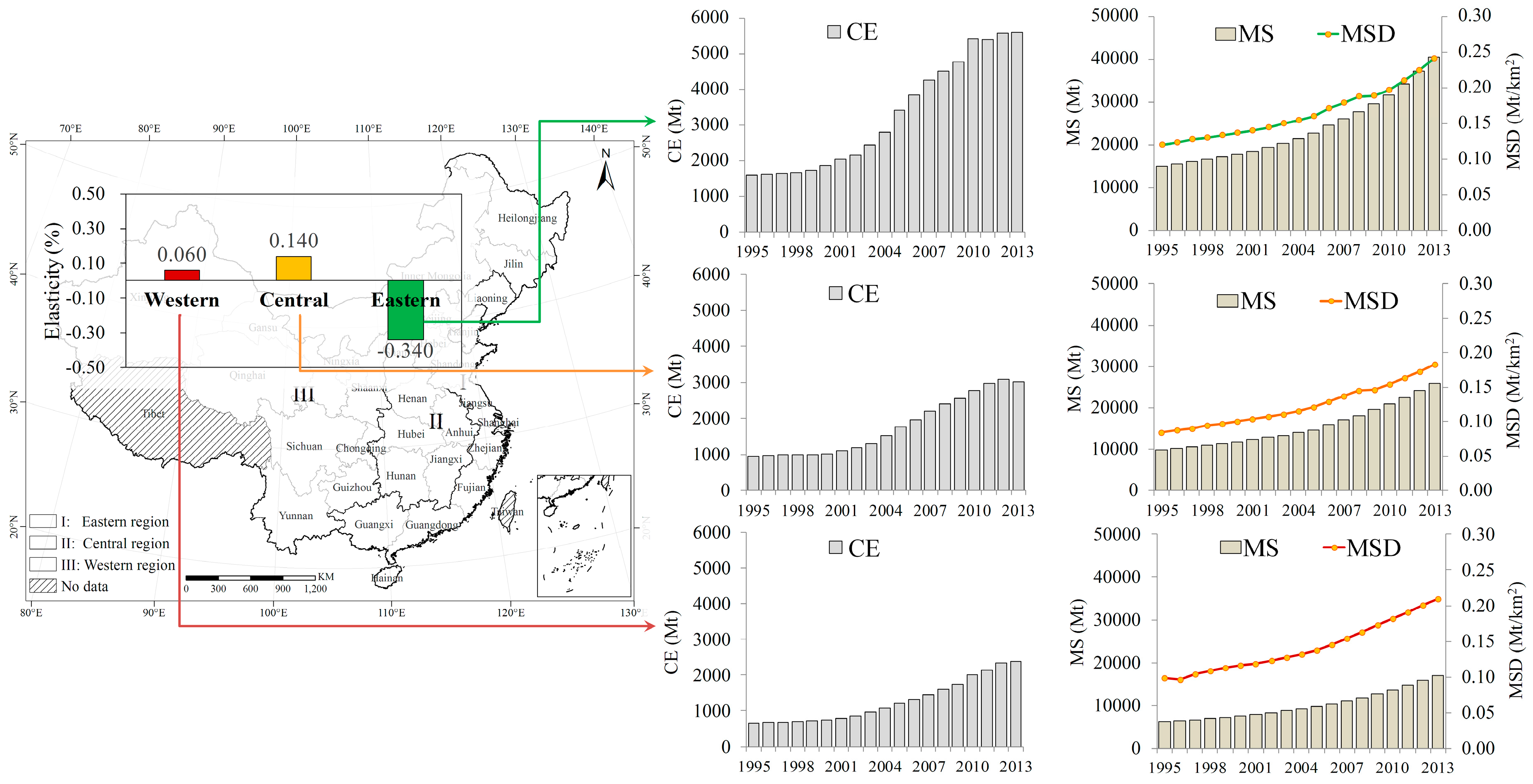
At the regional level, the effects of socioeconomic driving factors on CO2 emissions differ across regions. In the eastern region, the most important driving factor was GDP per capita, whose elasticity was 1.56. For the quadratic form of GDP per capita, only the eastern region showed a significant negative correlation with emissions, which suggested that as economic development continues, the CO2 emissions might peak and decline, exhibiting an inverted-U-shape trend. In the central and western regions, it was population that played the dominant role in affecting CO2 emissions, whose elasticity was 1.77 for the western region and 1.17 for the central region. The impact of the share of industry on CO2 emissions was positive in all the three regions but was smallest in the eastern region. This is mainly because of the relatively stable share of industry in GDP in Eastern China during the last 18 years. In 2013, the eastern region decreased its share of industry in GDP by only 1.16% compared to 1995, whereas the share of industry in GDP in the central and western regions increased from 41.47% and 39.97% to 51.08% and 48.96%, respectively, showing an increase of 9.61% and 9.65% compared to 1995. It is also interesting to find that the impact of material stocks density on CO2 emissions also varied across regions. As suggested in Table 5, a 1% increase in material stocks’ density will reduce CO2 emissions in the eastern region by 0.34% if all other factors remain stable. In contrast, it will increase CO2 emissions in the central and western regions by 0.14% and 0.06%, respectively.
3.3. Discussion and Policy Implications
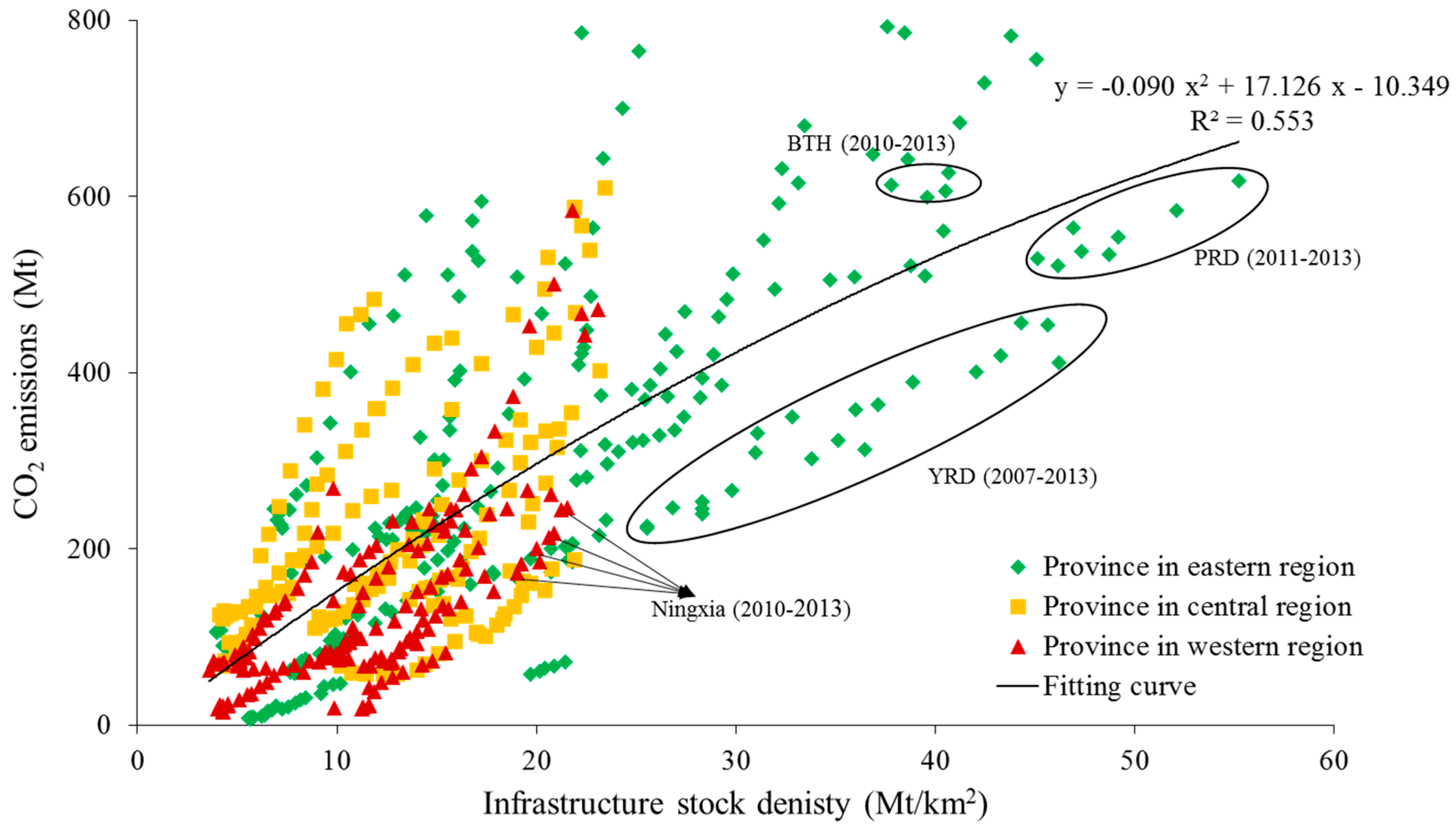
Generally, maintaining the economic growth at a medium-to-fast speed and at the same time reducing CO2 emissions are two primary challenges faced by China’s government. However, China is a broad country with big regional differences in its socio-economy and environment. In the past decades, though many favorable policies, such as the “Grand Western Development Program” and the “Rise of Central China Plan”, have been implemented by the central government to accelerate the development of the central and western regions, big gaps still exist across regions. Taking economic output as an example, in 2013, per capita GDP in the eastern region was 41,397 yuan RMB, which is 1.8 and 2.1 times of that in the central and western regions, respectively. Moreover, as shown in Figure 3, the total amount and growing speed of CO2 emissions and material stocks also varied per region. If we map the correlation between CO2 emissions and material stock density of each province from 1995 to 2013 (Figure 4), it is interesting to find that with the increase of material stock density CO2 emissions demonstrated an inverted-U-shape changing path (the R2 of fitting curve is around 0.6). Provinces in the western and central regions were located around the increasing part of the inverted-U-shape curve, where the infrastructure stock density was relatively low (ranging from 4.39 to 21.93 Mt/km2) while CO2 emissions were high. In contrast, provinces in the eastern region were located close to the turning point of the inverted-U-shape curve, where some provinces had relatively high stock density but relatively low emissions, and some had relatively high stock density but high emissions. Obviously, instead of a uniformed policy, region-based policies considering both the national strategic needs and local socio-economic and environmental situations should be paid much attention so as to forward the transition of the three sub-regions toward a low-carbon development.
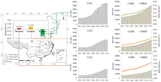
Figure 3.
Elasticity of CO2 emissions to material stocks density of infrastructure.

Figure 4.
CO2 emissions vs. infrastructure stock density at provincial level 1995–2013. Note: YRD (Yangtze River Delta) includes Shanghai, Jiangsu, and Zhejiang provinces; BTH includes Beijing, Tianjin, and Hebei provinces; PRD (Pearl River Delta) includes Guangdong province.
Specifically for the eastern region, to keep the spatial compactness of infrastructure stocks at a reasonable level would be an important implication for local governments in their infrastructure and urban planning. As indicated by Figure 3, both the absolute amount and density of infrastructure’s material stocks have reached a relatively high level in the eastern region, comparing to those in the central and western regions. It has also been confirmed by our panel analysis that the increase of infrastructure stock density will reduce CO2 emissions in the eastern region, which is consistent with the findings in many existing studies that a spatially compact urban form usually consumes less energy [9,37,38]. Moreover, as shown in Figure 4, in some highly urbanized areas such as Yangtze River Delta (YRD), Pearl River Delta (PRD), and Beijing-Tianjin-Hebei (BTH), their economic development has reached a high level and thus had a large amount of infrastructure stocks and high stock density. Meanwhile, they have also put a lot of efforts on developing low-carbon industries. For example, Guangdong province in PRD has been making great efforts to remove some heavy industries (such as chemical materials and metal smelting) and to promote the new energy vehicle industry in recent years [39]. Such experiences suggest that the upgrading and promoting the economic structure from carbon-intensive to low-carbon industries would be another important policy implications for the decision maker in this region.
For the central and western regions, though the extensive sprawl of urban built-up land and the rapid growth of infrastructure have been observed during the last decades [40], they are still in the relatively primary stage of development. The population size was larger in these two regions, while the population density was much smaller than the eastern region, which may result in the distribution of infrastructure stocks being relatively dispersed and prevent the intensive utilization of infrastructure. In 2013, the infrastructure stock density in the central and western regions was 0.18 and 0.21 Mt/km2, which was only 76% and 87% of that in the eastern region, respectively. This sprawl-type development with low infrastructure stock density in central and western regions not only indicates that the infrastructure in these regions are far from intensive utilization, but also limit the efficiency of material use and cause the rise of energy consumption and carbon emissions. In addition, due to the significant industrial transfer, which is promoted by the national and local governments as an important countermeasure to reduce the regional economic disparity [41], enormous resource and labor-intensive industries were transferred from eastern to inland areas since 2008. Certainly, it has accelerated the socio-economic development of those less developed regions, however it also stimulated the construction of infrastructure that provide services for carbon-intensive industries, which finally exacerbates CO2 emissions of these regions. In addition to raise the infrastructure stock density, at least two policy implications should be given emphasis for the policy makers in these two regions. First is to accelerate the development of renewable energy infrastructure. It is quite feasible and suitable to develop renewable energy infrastructure in provinces with rich clean energy resources and less densely populated areas [42,43]. As shown in Figure 4, Ningxia is a good example, as it had relatively low CO2 emissions but relatively high infrastructure stock density, as it has been making vast investment on solar and wind power. By 2012, the capacity of wind power and solar power has reached 2 million KW and 0.5 million KW respectively, which makes Ningxia one of the most rapidly growing provinces in exploiting renewable energy in China [44]. Moreover, the local government may also promote the use of Power-to-Gas technology, which are sustainable and will produce only about 20% of greenhouse gases than fossil fuel [45,46]. By doing these, it could be a good opportunity for the inland regions to get on the path of technological innovation, attract high-tech enterprise, and eventually realize green industrial upgrading. The second implication is to construct and utilize infrastructure in an energy-efficient way. Since more infrastructure will be constructed in the central and western regions as the urbanization rate is expected to continuously increase in the future decades, reducing or replacing the construction materials of infrastructure from high-carbon-footprint ones (such as steel, cement, and lime) to less carbon-intensive ones (such as aluminum alloy and nano-materials) could be an effective option for CO2 mitigation. Additionally, equipping infrastructure with more energy-saving facilities would also be important to cut CO2 emissions during its in-use life stage.
4. Conclusions
Because of the important roles of infrastructure in shaping the socio-economic and climate change paths, it is necessary to incorporate infrastructure stocks into the driving force analysis of CO2 emissions so that effective policies could be designed to direct the infrastructure development in a low-carbon and sustainable way. Based on the accounting of the CO2 emissions and material stocks in infrastructure of Chinese provinces, we investigated the impact of socioeconomic development especially the effect of infrastructure stocks on CO2 emissions in China. The main findings are summarized as follows:
First, at country level, population was the most important factor, followed by GDP per capita and energy intensity in affecting CO2 emissions. It is also confirmed by our study that the accumulation of materials in infrastructure do have an impact on CO2 emissions, for which every 1% increase in material stocks per built-up area would lead to a 0.11% decrease in CO2 emissions if other driving factors remain unchanged.
Second, at the regional level, the effect of driving factors on CO2 emissions varied across regions. In the eastern region, emissions were mainly driven by GDP per capita and showed an inverted-U-shape trend when economy continues to growth. In the central and western regions, population was the most important determinant of CO2 emissions. Infrastructure stocks had a negative correlation with CO2 emissions in the eastern region (with elasticity of −0.34), but a positive correlation in the central and western regions (with its elasticity of 0.06 and 0.14, respectively).
Third, since high material stocks density would result in a significant reduction of CO2 emissions, it is crucial to improve the spatial compactness of infrastructure stocks when increasing the total amount of infrastructure in the future. Region-based policy implications include upgrading the economic structure to a low-carbon one for the eastern region, accelerating the development of renewable energy infrastructure, and replacing high carbon footprint materials to less carbon-intensive ones; and increasing the utilization of energy-saving facilities during the in-use phase of infrastructure for the central and western regions.
Acknowledgments
This research was supported by the National Key Research and Development Program of China (grant number 2017YFC0505703); the National Natural Science Foundation of China (grant number 41401638, 41471076), the Shanghai Philosophy and Social Sciences Planning Project (grant number 2014BCK001), and the China Ministry of Education’s Humanities and Social Sciences Project (grant number 14YJAZH028).
Author Contributions
Ji Han designed the research and revised the manuscript. Xing Meng performed the calculations, analyzed the results, and wrote the draft. Jiabin Liu and Yanqi Zhang contributed to the result analysis and paper writing.
Conflicts of Interest
The authors declare no conflict of interest.
References
- Liu, G.; Bangs, C.E.; Muller, D.B. Stock dynamics and emission pathways of the global aluminium cycle. Nat. Clim. Chang. 2013, 3, 338–342. [Google Scholar] [CrossRef]
- Muller, D.B.; Liu, G.; Lovik, A.N.; Modaresi, R.; Pauliuk, S.; Steinhoff, F.S.; Brattebø, H. Carbon Emissions of Infrastructure Development. Environ. Sci. Technol. 2013, 47, 11739–11746. [Google Scholar] [CrossRef] [PubMed]
- Lucon, O.; Ürge-Vorsatz, D.; Zain Ahmed, A.; Akbari, H.; Bertoldi, P.; Cabeza, L.F.; Eyre, N.; Gadgil, A.; Harvey, L.D.D.; Jiang, Y.; et al. Buildings. In Climate Change 2014: Mitigation of Climate Change; Contribution of Working Group III to the Fifth Assessment Report of the Intergovernmental Panel on Climate Change; Cambridge University Press: Cambridge, UK; New York, NY, USA, 2014; Available online: http://www.ipcc.ch/pdf/assessment-report/ar5/wg3/ipcc_wg3_ar5_chapter9.pdf (accessed on 29 July 2017).
- Seto, K.C.; Dhakal, S.; Bigio, A.; Blanco, H.; Delgado, G.C.; Dewar, D.; Huang, L.; Inaba, A.; Kansal, A.; Lwasa, S.; et al. Human Settlements, Infrastructure and Spatial Planning. In Climate Change 2014: Mitigation of Climate Change; Contribution of Working Group III to the Fifth Assessment Report of the Intergovernmental Panel on Climate Change; Cambridge University Press: Cambridge, UK; New York, NY, USA, 2014; Available online: http://www.ipcc.ch/pdf/assessment-report/ar5/wg3/ipcc_wg3_ar5_chapter12.pdf (accessed on 29 July 2017).
- United Nations. World Urbanization Prospect: The 2014 Revision; United Nations: New York, NY, USA, 2015; Available online: https://esa.un.org/unpd/wup/Publications/Files/WUP2014-Report.pdf (accessed on 29 July 2017).
- Van Vuuren, D.P.; Stehfest, E.; den Elzen, M.G.J.; Kram, T.; van Vliet, J.; Deetman, S.; Isaac, M.; Goldewijk, K.K.; Hof, A.; Beltran, A.M.; et al. RCP2.6: Exploring the possibility to keep global mean temperature increase below 2 °C. Clim. Chang. 2011, 109, 95. [Google Scholar] [CrossRef]
- Poumanyvong, P.; Kaneko, S. Does urbanization lead to less energy use and lower CO2 emissions? A cross-country analysis. Ecol. Econ. 2010, 70, 434–444. [Google Scholar] [CrossRef]
- Sharma, S.S. Determinants of carbon dioxide emissions: Empirical evidence from 69 countries. Appl. Energy 2011, 88, 376–382. [Google Scholar] [CrossRef]
- Fang, C.L.; Wang, S.J.; Li, G.D. Changing urban forms and carbon dioxide emissions in China: A case study of 30 provincial capital cities. Appl. Energy 2015, 158, 519–531. [Google Scholar] [CrossRef]
- Yang, W.; Li, T.; Cao, X. Examining the impacts of socio-economic factors, urban form and transportation development on CO2, emissions from transportation in China: A panel data analysis of China’s provinces. Habitat. Int. 2015, 49, 212–220. [Google Scholar] [CrossRef]
- Liu, Y.; Wang, Y.; Huo, H. Temporal and spatial variations in on-road energy use and CO2 emissions in China, 1978–2008. Energy Policy 2013, 61, 544–550. [Google Scholar] [CrossRef]
- Lin, C.; Liu, G.; Müller, D.B. Characterizing the role of built environment stocks in human development and emission growth. Resour. Conserv. Recycl. 2017, 123, 67–72. [Google Scholar] [CrossRef]
- Han, J.; Xiang, W.N. Analysis of material stock accumulation in China’s infrastructure and its regional disparity. Sustain. Sci. 2013, 8, 553–564. [Google Scholar] [CrossRef]
- Pauliuk, S.; Müller, D.B. The role of in-use stocks in the social metabolism and in climate change mitigation. Glob. Environ. Chang. 2014, 24, 132–142. [Google Scholar] [CrossRef]
- Shi, P.J.; Yu, D.Y. Assessing urban environmental resources and services of Shenzhen, China: A landscape-based approach for urban planning and sustainability. Landsc. Urban Plan. 2014, 125, 290–297. [Google Scholar] [CrossRef]
- National Bureau Statistics of the People’s Republic of China. China Statistical Yearbook 2016; National Bureau Statistics of China: Beijing, China, 2016. Available online: http://www.stats.gov.cn/tjsj/ndsj/2016/indexch.htm (accessed on 29 July 2017).
- U.S. Geological Survey. Mineral Commodity Summaries; USGS: Sioux Falls, SD, USA, 2014. Available online: http://minerals.usgs.gov/minerals/pubs/commodity/cement/mcs-2014-cemen.pdf (accessed on 29 September 2017).
- Davis, S.J.; Caldeira, K.; Matthews, H.D. Future CO2 emissions and climate change from existing energy infrastructure. Science 2010, 329, 1330–1333. [Google Scholar] [CrossRef] [PubMed]
- The Intergovernmental Panel on Climate Change (IPCC). Climate Change 2007: The Physical Science Basis; Cambridge University Press: Cambridge, UK, 2007. [Google Scholar]
- Meng, X.; Han, J.; Huang, C. An improved vegetation adjusted nighttime light urban index and its application in quantifying spatiotemporal dynamics of carbon emissions in China. Remote Sens. 2017, 9, 829. [Google Scholar] [CrossRef]
- National Bureau Statistics of China. China Energy Statistical Yearbook; China Statistics Press: Beijing, China, 1996–2014.
- Muller, D.B. Stock dynamics for forecasting material flows: Case study for housing in The Netherlands. Ecol. Econ. 2006, 59, 142–156. [Google Scholar] [CrossRef]
- Gerst, M.D. Linking material flow analysis and resource policy via future scenarios of in-use stock: An example for copper. Environ. Sci. Technol. 2009, 43, 6320–6325. [Google Scholar] [CrossRef] [PubMed]
- Krausmann, F.; Richter, R.; Eisenmenger, N. Resource use in small island states: Material flows in Iceland and Trinidad and Tobago, 1961–2008. J. Ind. Ecol. 2014, 18, 294–305. [Google Scholar] [CrossRef] [PubMed]
- Huang, C.; Han, J.; Chen, W.Q. Changing patterns and determinants of infrastructures’ material stocks in Chinese cities. Resour. Conserv. Recycl. 2016, 123, 47–53. [Google Scholar] [CrossRef]
- Ehrlich, P.R.; Holdren, J.P. Impact of population growth. Science 1971, 171, 1212–1217. [Google Scholar] [CrossRef] [PubMed]
- Dietz, T.; Rosa, E.A. Rethinking the environmental impacts of population, affluence, and technology. Hum. Ecol. Rev. 1994, 1, 277–300. [Google Scholar]
- Dietz, T.; Rosa, E.A. Effects of population and affluence on carbon dioxide emissions. Proc. Natl. Acad. Sci. USA 1997, 94, 175–179. [Google Scholar] [CrossRef] [PubMed]
- York, R. Asymmetric effects of economic growth and decline on CO2 emissions. Nat. Clim. Chang. 2012, 2, 762–764. [Google Scholar] [CrossRef]
- Granger, C.W.J.; Newbold, P. Spurious regressions in econometrics. J. Econ. 1974, 2, 111–120. [Google Scholar] [CrossRef]
- Gutierrez, L. On the power of panel cointegration tests: A Monte Carlo comparison. Econ. Lett. 2003, 80, 105–111. [Google Scholar] [CrossRef]
- Pedroni, P. Panel cointegration: Asymptotic and finite sample properties of pooled time series tests with an application to the PPP hypothesus. IDEAS 2004, 20, 597–625. [Google Scholar] [CrossRef]
- Wooldridge, J.M. Econometric Analysis of Cross Section and Panel Data; MIT Press: Cambridge, UK, 2002. [Google Scholar]
- Du, G.Y.; Cai, Y.L.; Li, S.C. Fossil-fuel carbon emission intensity change of each province in China during 1997–2007. Geogr. Inf. Sci. 2010, 26, 76–81. (In Chinese) [Google Scholar]
- Liu, Y.C. Land Resources Survey Data sets of China; National Land Resource Survey Office: Beijing, China, 2000. (In Chinese)
- Wang, S.; Fang, C.; Wang, Y. Spatiotemporal variations of energy-related CO2 emissions in China and its influencing factors: An empirical analysis based on provincial panel data. Renew. Sustain. Energy Rev. 2016, 55, 505–515. [Google Scholar] [CrossRef]
- Hankey, S.; Marshall, J.D. Impacts of urban form on future us passenger-vehicle greenhouse gas emissions. Energy Policy 2010, 38, 4880–4887. [Google Scholar] [CrossRef]
- Makido, Y.; Dhakal, S.; Yamagata, Y. Relationship between urban form and CO2 emissions: Evidence from fifty Japanese cities. Urban Clim. 2012, 2, 55–67. [Google Scholar] [CrossRef]
- Chip Card Interface Device (CCID). Consulting 2011: The White Paper of New Energy Industry Maps in China; CCID: Beijing, China; Available online: http://data.ccidconsulting.com/ei/bps/xny/H681104index_1.htm (accessed on 24 May 2016). (In Chinese)
- Deng, X.; Zhan, J.; Rui, C. The patterns and driving forces of urban sprawl in China. IEEE Int. Geosci. Remote Sens. Symp. 2005, 3, 1511–1513. [Google Scholar]
- Ye, Q. The transfer trend and undertaking competitive situation of China’s regional industry. Econ. Geogr. 2016, 34, 91–97, (In Chinese with English Abstract). [Google Scholar]
- Rovense, F.; Perez, M.S.; Amelio, M.; Ferraro, V.; Scornaienchi, N.M. Feasibility analysis of a solar field for a closed unfired joule-brayton cycle. Int. J. Heat. Technol. 2017, 35, 166–171. [Google Scholar] [CrossRef]
- Noussan, M.; Jarre, M.; Poggio, A. Real operation data analysis on district heating load patterns. Energy 2017, 129, 70–78. [Google Scholar] [CrossRef]
- Ningxia has become the first comprehensive new energy demonstration area in China. China News. 17 September 2012. Available online: http://finance.chinanews.com/ny/2012/09-17/4189004.shtml (accessed on 3 December 2017). (In Chinese).
- Thamsiriroj, T.; Smyth, H.; Murphy, J.D. A roadmap for the introduction of gaseous transport fuel: A case study for renewable natural gas in Ireland. Renew. Sustain. Energy Rev. 2011, 15, 4642–4651. [Google Scholar] [CrossRef]
- Nastasi, B.; Basso, G.L. Power-to-gas integration in the transition towards future urban energy systems. Int. J. Hydrogen Energy 2017, 42, 23933–23951. [Google Scholar] [CrossRef]
© 2017 by the authors. Licensee MDPI, Basel, Switzerland. This article is an open access article distributed under the terms and conditions of the Creative Commons Attribution (CC BY) license (http://creativecommons.org/licenses/by/4.0/).

