Oil Price and Economic Resilience. Romania’s Case

Abstract

The emerging economies that do not face fiscal, monetary and foreign debt pressures can use the savings generated by lower oil prices for investments in order to generate economic growth. Hence, there is no doubt that the oil price affects the economy’s resilience to shocks. The importance of this impact derives from the magnitude of the price change and its diffusion within the economy. Moreover, the sustainability of any company and of the economy as a whole is subject to the availability and the price of the energy resources. The cost of these resources is an important variable used in the majority of the models regarding the assessment of sustainable development. Therefore, this article examines the impact of the oil price changes on industrial production in Romania. We found that, similar to other countries, in Romania, the growth rate of industrial production responds more strongly to a rise in oil prices. Thus, the oil Brent price has an asymmetric effect on the production evolution. This finding suggests that macroeconomic stabilization is more difficult to achieve when the oil price rises.

1. Introduction

The impact of oil prices on the main macroeconomic variables—economic growth, inflation and unemployment—represents an important economic issue. It is generally acknowledged that the oil price affects industrial production and the economy’s resilience to shocks. However, the impact depends on the size of the price amendments and their propagation within the economy. The aim of this article is to investigate the impact of the oil Brent price changes on industrial production in Romania.

The relationship between the oil price and real GDP growth constitutes the subject of numerous articles [1,2,3,4] and, regardless of the research methodology, the general conclusion is that the rate of economic growth is adversely affected by the increase of the oil prices. Burbidge and Harrison [5] used the auto-regression vector (VAR) methodology to analyse how industrial production was influenced by the oil price in the US, Japan, the Federal Republic of Germany, the United Kingdom (UK), and Canada for the period of 1961–1982. They concluded that the oil price had a considerable influence on the industrial production only in the US and UK. Hamilton [6] analysed the influence of oil prices on GDP evolution. He employed a nonlinear regression model to demonstrate that there is a negative relationship between the quarterly growth rate of chain-weighted real GDP and the nominal crude oil producer price index, seasonally unadjusted. He showed that the fall of oil prices is not as important for predicting the evolution of the GDP as the price increase. Zhang [7] applied a methodology similar to the one employed by Hamilton (2003) on the case of Japan for the period 1957 Q1–2006 Q4. He concluded that divergent changes in oil prices affected the economy of Japan in different ways. The impact of a price increase was higher than the influence of a price decrease. Romero-Meza et al. [8] used monthly data for the period of 1974–2013 in order to demonstrate that oil prices affect industrial production in the US, production that is considered as a proxy for the real GDP. An International Monetary Fund (IMF) report [9] emphasized that the growing scarcity of oil can affect global growth: a reduction by 1% in the oil supply might slow down the global GDP growth by approximately 0.25% on medium and long term. The negative shock in the long-run growth occurs even when the price elasticity of the demand in oil rises due to an increased use of substitutes.

The asymmetrical influence of the oil prices on the economic growth was also demonstrated by Engemann et al. [10]. They showed that the size of the oil price shock on the payroll employment, used as proxy for GDP growth, was dependent on the characteristics of each US state. Furthermore, the asymmetry was confirmed by the study of Serletis and Istiak for Canada, Germany, Italy and Japan [11], and by Cunado and Perez de Gracia, through their study of 15 European countries [12]. Federed [13] and Elder and Serletis [14] concluded that the volatility of the oil price affects the growth of the real GDP in a negative way. Hooker [15] demonstrated that, since 1974, the macroeconomic influence of the oil price has been gradually decreasing. Kilian estimated the effects of exogenous shocks on inflation and real output in the G7 countries (United States, Italy, France, Germany, UK, Canada and Japan) and compared them to global oil production. He concluded that, depending on the period of shocks to the oil supply, they have little to no impact on real growth in most of the G7 countries [16].

According to Husain et al. [17], the macroeconomic impact of the oil price decrease is determined by its magnitude and by its spread within the oil product prices and within domestic end-user prices. Correspondingly, a significant reduction in oil prices (i.e., 40% in 2015) might have the potential to determine, within a two-year period, the increase of the global GDP by 0.5% (excepting the petroleum-exporting countries). They suggest that the oil-importing countries, including the emerging economies, should invest the income generated by the decrease in the oil price with the aim of generating economic growth.

Bumpass et al. studied the relationship between the retail gasoline price and the spot oil price, as well as the wholesale gasoline price and the spot oil price with threshold autoregressive TAR models [18]. They concluded that the gasoline price responds asymmetrically to oil price changes over a longer period of time and the gasoline retailers and wholesalers have very little to no market power in the long term.

The rest of the paper is organized into two sections. The first and next section describes the analysed data and the generated results. The second and last section presents the conclusions of our study.

2. Data and Results

This article analyses the impact of the oil Brent price on industrial production in Romania by using monthly data for the period of January 2008–July 2016. We used monthly data for the crude oil price per litre [19] and for industrial production in Romania [20].

The variables used in the analysis are: y = percentage change in industrial production, x₁ = percentage change in oil Brent price, x₂ = positive percentage change in oil Brent price, x₃ = negative percentage change in oil Brent price.

2.1. Co-Integration Test Results

In this subsection, we use co-integration tests [21,22] to examine the co-integration relationship between industrial production and the oil Brent price.

In order to analyse the co-integration relationship between two-time series (industrial production and the oil Brent price), we had to test if the two-data series are stationary. For this evidence, we used the Augmented Dikey-Fuller (ADF) test [23] and the Phillips-Peron (PP) [24] test.

• H₀: the series have/has unit root (the series are/is non-stationary)
• H₁: series are/is stationary

The results of the ADF and PP tests are shown in

Table 1. Integration test.

	Test Augment Dikey-Fuller	Probability	Test Phillips-Peron	Probability
LEVEL
y	−1.6	0.47	−2.86	0.05
x1	−8.48	0.000	−8.51	0.0000
FIRST DIFFERENCE
y	−17.46	0.000	−19.63	0.000
x1	-	-	-	-
Test critical values: 1% (−3.49); 5% (−2.89); 10% (−2.58)

. Accordingly, the percentage change of the Brent quotation was stationary, while the percentage change of the industrial production was stationary at its first difference.

Figure 1 shows the stationarity of the industrial production and the oil Brent price at their first difference.

Next, we used the Engle-Granger test and the Johansen test to investigate the existence of a long-term, balanced relationship between the percentage change of industrial production and the percentage change of the oil Brent price.

Using the Engle-Granger test implies a three-stage process:

(1)

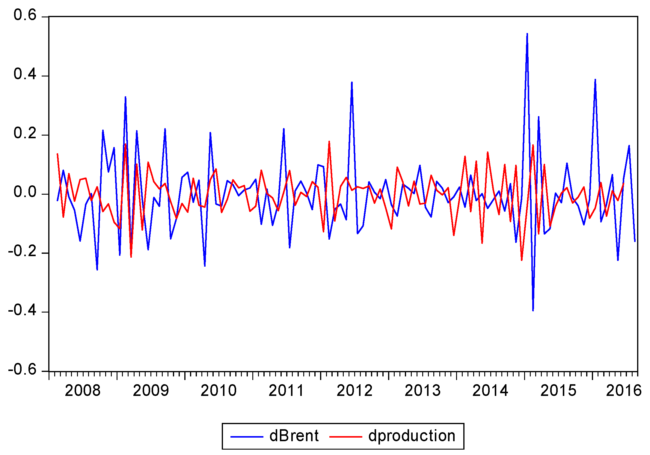
Determining the integration order of the variables. In the first part of the paper we analysed the integration order of the two variables used (y and x₁) in our analysis. Since the data series have to have the same integration order, we will use the integration order 1 (first difference) for both variables (because the Brent quotation is stationary on the first level, while the percentage change of the industrial production is stationary at its first difference).

(2)

Estimating the long-run (equilibrium) equation:

$$y_{\mathrm{t}}= {\beta }_0+{\beta }_1{x}_{1t}+{\epsilon }_t,$$

(1)

where $\epsilon$ is the error term; $y_t$ is the percentage change of the industrial production integrated by order 1; $x_1$ is the percentage change of the oil Brent price integrated by order 1; and t is the time trend. The ordinary least squares (OLS) residuals from Equation (1) are a measure of the imbalance:

$$u_t=y_t-\left(\widehat{{\beta }_0}+\widehat{{\beta }_1}{x}_1\right)$$

(2)

We must check if the residuals of Equation (2) are stationary. The simple linear regression model (Equation (1)) was statistically valid because Prob (F-statistic) = 0.03 was less than 0.05, and the residuals were normally distributed (the Jarque-Bera probability was 65%, showing that the null hypothesis cannot be rejected). We used the ADF test to validate the stationarity of the residuals. The results of the ADF test showed that the residuals are stationary (t_ADF < t_{calculate (1%, 5%, 10%)} and the associated probability (0.0001) is smaller than 0.05), meaning that y and x₁ have a long equilibrium relationship.

(3)

As the variables y and x₁ are co-integrated, we estimated the ECM (error correction model) as shown below:

$$\Delta y={\beta }_2+{\beta }_3\Delta x_1+{\beta }_4{u}_{t-1}+v$$

(3)

where ${\beta }_2$ is the intercept, ${\beta }_3$ is the short-run coefficient, v is the white noise error term, and $u_{t-1}$ is an error correction term that guides the variables (y and x₁) of the system to restore the balance. In our case, the coefficient ${\beta }_4$ was negative (−1.48) and statistically significant (the probability of this coefficient was less than 1%). In this case, between y and x₁ there is a long-term, balanced relationship. We can state that the industrial production adjusts in a current month as a consequence of a past monthly imbalance. We used the Jarque-Bera test to test for the normal distribution of the ECM residuals. It showed that the residuals were normally distributed (the Jarque-Bera test probability was 25%).

The Johansen test provides information regarding the number of integration relations within a model. It can be conducted in two ways: the trace test and the maximum eigenvalue test. Both forms of the test examine the number of linear combinations. The null hypotheses (H₀) is K = 0, meaning no integration, but the alternative hypothesis is K greater than 0 for the test trace and k + 1 for the maximum eigenvalue.

In

Table 2. The long-term relationship between the industrial production and the oil Brent price.

	Eigen Value	Trace Statistic	0.05 Critical Value	Max—Eigen Statistic	Probability
None	1.0000	3544.56	15.49	1.0000	1.0000
At most 1	0.169	17.83	3.84	0.1695	0.000
	Eigen Value	Trace Statistic	0.05 Critical Value	Max—Eigen Statistic	Probability
None	1.0000	3526.73	14.26	1.0000	1.0000
At most 1	0.169	17.83	3.84	0.1695	0.0000

we rejected the null hypothesis of no co-integration and established the presence of one co-integration equation based on the trace and maximum eigenvalue statistics. We selected the lag for the Johansen test with the lag length criteria test.

2.2. VECM (Vector Error Correction) Analysis

In this subsection, we estimated the percentage of imbalances within the industrial output due to the oil Brent price changes by using the VECM (vector of errors correction method) [25]. VECM is a representation of VAR with restrictions. The general form of the VECM model is:

$$\Delta Y_t=\Phi Y_{t-1}+{\Gamma }_1\Delta Y_{t-1}+\mathrm{...}+{\Gamma }_{p-1}\Delta Y_{t-p+1}+{\epsilon }_t,$$

(4)

where, $\Phi ={\displaystyle \sum _{i=1}^p{B}_i}-I$; I is the unit matrix; ${\Gamma }_i=-{\displaystyle \sum _{i=1}^p{B}_{i+1}}$, where B_i is the matrix corresponding to the associated coefficients Y_t-I; $Y_t=A+B_1{Y}_{t-1}+B_2{Y}_{t-2}+\mathrm{...}+B_p{Y}_{t-p}+{\epsilon }_t$ is a VAR(p) of order p, where y_t is an n × 1 vector of variables that are integrated of order one—commonly denoted I(1)—ε_t is an n × 1 vector of innovations and t is time.

The VECM equation can be written as follows:

$$y_t=0.006+0.77y_{t-1}+0.101y_{t-2}-0.35{\epsilon }_{t-1}-0.14{\epsilon }_{t-2}-0.067b,$$

(5)

where y_t = the percentage change of the industrial production integrated by order one at time t; y_t−1, y_t−2, ..., y_t−n is the percentage change of the industrial production integrated by order one at time t − 1, t − 2,…, t − n; b is the percentage change of the oil Brent price integrated by order one; ${\epsilon }_{t-1, t-2}$ is the residual at time t − 1 and t − 2.

The equation above shows that there is a positive correlation between the industrial production and its previous monthly value (0.77), and a negative correlation between the industrial production and the oil Brent price (−0.067). About 0.35 of the monthly imbalances in the production levels are corrected by the oil Brent price changes.

2.3. Asymmetry Tests

We tested the asymmetry between an increasing or decreasing oil Brent price and the industrial production using the TAR model [26] and Wald tests [27].

In order to run the two tests, we estimated the following regression equation:

Y_it = ß₀ + ß₁ X_2t + ß₂ X_3t + Ɛ_it, i = 1…N, t = 1…T,

(6)

where, i is variable and t is time, X₂ = positive percentage change in the oil Brent price integrated by order one, X₃ = negative percentage change in the oil Brent price integrated by order one.

Thus, the regression equation is:

$$y={0.11}_{\begin{array}{c}1\\ \left(-1,004\right)\\ 0.31\end{array}}-0.18x_{\begin{array}{c}\begin{array}{c}2\\ \left(-2,3\right)\end{array}\\ 0.02\end{array}}+0.16x_{\begin{array}{c}3 \\ \left(1,7\right)\\ 0.009\end{array}}\left(-6\right)-0.49 y{\left(-1\right)}_{\begin{array}{c}\left(-5,5\right)\\ \left(0,000\right)\end{array}},$$

(7)

R² = 0.28

The model is statistically valid because Prob (F-statistic) is 0.0000. To validate the regression equation we included another exogenous variable, y(−1). It shows the percentage change of the industrial production integrated by order one for the last month. For x₃ we used a six-month lag.

The values inside the parentheses are the standard errors. The variables used are statistically significant, whereas the probability associated with each variable is less than 1% (except the constant). To check the model’s validity, we used the following tests:

-

the Lagrange Multiplier (LM) test for serial correlation. It showed there is no serial correlation in the residual (because of this we used a one-period lag of the dependent variable);

-

the Jarque-Bera test for the normality of the residuals (the probability was 35%, showing that the null hypothesis cannot be rejected);

-

the White test for heteroskedasticity;

-

the augmented Dickey-Fuller (ADF) test for stationarity of the variables. The y, x₂, and x₃ variables are integrated by order one. All tests showed that the results of the regression equation are valid.

The regression equation showed that industrial production is negatively affected by an increase in the price of the oil and positively influenced by a decrease of the oil price with a six-month lag.

We used a TAR model to examine how industrial production responds to the imbalances of the oil Brent price. In

Table 3. TAR test.

Variable	Coefficient	T-Statistic	Probability	Std. Error
Increase (X2)	−0.14	−2.38	0.016	0.09
Decrease (X3) (lag 6)	0.23	2.33	0.0217	0.11

the probability of an increase in the Brent price was 0.016, which is lower than 0.5, and the probability of a decrease in the Brent price (with a lag of six months) was 0.0217. Thus, the model is statistically valid. At T-6, the response of the production change to the oil Brent price evolution is asymmetrical. The current value of the production is very sensitive to its previous values, especially to T-6, considering that its monthly value tends to respond significantly even to infinitesimal changes of the Brent price.

To test the restrictions of the parameters that we used in the model (increase/decrease of the Brent price), we used the Wald test,

Table 4. Wald test.

Test Statistic	Value	Probability
t-statistic	−0.46	0.64
F-Statistic	0.213	0.64
Chi-square	0.213	0.64
Null Hypothesis: c(1) = c(2)

. In this test we used the following null hypothesis: H₀: c(1) = c(2), where c(1) shows the coefficient corresponding to an increase in the Brent price, while c(2) shows the coefficient when the Brent price decreases. The null hypothesis is determined by the regression equation and the TAR model. The TAR model indicates that the change of the Brent quotation has a different impact on the industrial production. The Wald test checks if the two independent variables (X₂ and X₃) have different influences on industrial production.

The Wald test rejected the null hypothesis, since F (static) was 0.213. Thus, the change of the oil Brent price affects the industrial production differently. Moreover, the production can be quickly adjusted when the Brent price rises (Table 4).

3. Conclusions

This article showed that there is a long-term equilibrium relationship between the industrial production and the oil Brent price, implying that the two-data series are co-integrated. The monthly variation of the industrial production is positively correlated with its previous monthly value and negatively correlated with the oil Brent price. This finding is consistent with the results of previous studies [10]. The two variables (the Brent price increase and decrease) affect industrial production in a different way. The impact of an increase in the Brent price on the industrial production variation is faster than the impact in the case of a decrease in the Brent price. Moreover, the decrease was observed with a six-month lag. Therefore, there is an asymmetric influence of the oil Brent price on the industrial production adjustment. This result confirms the hypothesis of asymmetry and demonstrates that the oil prices affect economic growth, as was previously demonstrated in other studies [6,7,11,12].

The oil price change explains less than 30% of the industrial production change. Therefore, oil shocks (such as the one in 1973) do not fully explain the worldwide economic recessions associated with them. The oil price increase generates the deterioration of the external investment position of an oil import–dependent country. Alternatively, the respective country will experiment with a budgetary surplus when the oil price decreases. The budgetary surplus can be used for decreasing the foreign public debt burden. Romania, a country with a low level of indebtedness compared to the European average, should use the incomes obtained from the decrease in the oil price to stimulate economic growth.

References

- Gisser, M.; Goodwin, T.H. Crude oil and the macroeconomy: Tests of some popular notions: Note. J. Money Credit Bank. 1986, 18, 95–103. [Google Scholar] [CrossRef]
- Dotsey, M.; Reid, M. Oil shocks, monetary policy, and economic activity. FRB Richmond Econ. Rev. 1992, 78, 14–27. [Google Scholar]
- Brown, S.P.; Yücel, M.K. Energy prices and aggregate economic activity: An interpretative survey. Q. Rev. Econ. Financ. 2002, 42, 193–208. [Google Scholar] [CrossRef]
- Aguiar-Conraria, L.; Wen, Y. Understanding the large negative impact of oil shocks. J. Money Credit Bank. 2007, 39, 925–944. [Google Scholar] [CrossRef]
- Burbidge, J.; Harrison, A. Testing for the effects of oil-price rises using vector autoregressions. Int. Econ. Rev. 1984, 25, 459–484. [Google Scholar] [CrossRef]
- Hamilton, J.D. What is an oil shock? J. Econ. 2003, 113, 363–398. [Google Scholar] [CrossRef]
- Zhang, D. Oil shock and economic growth in Japan: A nonlinear approach. Energy Econ. 2008, 30, 2374–2390. [Google Scholar] [CrossRef]
- Romero-Meza, R.; Coronado, S.; Serletis, A. Oil and the economy: A cross bicorrelation perspective. J. Econ. Asymmetr. 2014, 11, 91–95. [Google Scholar] [CrossRef]
- International Monetary Fund. World Economic Outlook. Tensions from the Two-Speed Recovery Unemployment, Commodities, and Capital Flows; International Monetary Fund: Washington, DC, USA, 2011; pp. 89–123. [Google Scholar]
- Engemann, K.M.; Owyang, M.T.; Wall, H.J. Where is an oil shock? J. Reg. Sci. 2014, 54, 169–185. [Google Scholar] [CrossRef]
- Serletis, A.; Istiak, K. Is the oil price–output relation asymmetric? J. Econ. Asymmetr. 2013, 10, 10–20. [Google Scholar] [CrossRef]
- Cuñado, J.; de Gracia, F.P. Do oil price shocks matter? Evidence for some European countries. Energy Econ. 2003, 25, 137–154. [Google Scholar] [CrossRef]
- Ferderer, J.P. Oil price volatility and the macroeconomy. J. Macroecon. 1997, 18, 1–26. [Google Scholar] [CrossRef]
- Elder, J.; Serletis, A. Oil price uncertainty. J. Money Credit Bank. 2010, 42, 1137–1159. [Google Scholar] [CrossRef]
- Hooker, M.A. What happened to the oil price-macroeconomy relationship? J. Monet. Econ. 1996, 38, 195–213. [Google Scholar] [CrossRef]
- Kilian, L. A comparison of the effects of exogenous oil supply shocks on output and inflation in the G7 countries. J. Eur. Econ. Assoc. 2008, 6, 78–121. [Google Scholar] [CrossRef]
- Husain, M.A.M.; Arezki, M.R.; Breuer, M.P.; Haksar, M.V.; Helbling, M.T.; Medas, P.A.; Sommer, M. Global Implications of Lower Oil Prices; No. 15; International Monetary Fund: Washington, DC, USA, 2015. [Google Scholar]
- Bumpass, D.; Ginn, V.; Tuttle, M.H. Retail and wholesale gasoline price adjustments in response to oil price changes. Energy Econ. 2015, 52, 49–54. [Google Scholar] [CrossRef]
- Ec.europa.eu. Available online: https://ec.europa.eu/energy/en/data-analysis/weekly-oil-bulletin (accessed on 29 August 2016).
- National Institute of Statistics. Available online: http://statistici.insse.ro/shop/?lang=en (accessed on 10 June 2016).
- Johansen, S. Statistical analysis of cointegration vectors. J. Econ. Dyn. Control 1988, 12, 231–254. [Google Scholar] [CrossRef]
- Engle, R.F.; Granger, C.W. Co-integration and error correction: Representation, estimation, and testing. Econom. J. Econ. Soc. 1987, 55, 251–276. [Google Scholar] [CrossRef]
- Dickey, D.A.; Fuller, W.A. Distribution of the estimators for autoregressive time series with a unit root. J. Am. Stat. Assoc. 1979, 74, 427–431. [Google Scholar] [CrossRef]
- Asteriou, D.; Hall, S.G. Applied Econometrics; Palgrave Macmillan: New York, NY, USA, 2015. [Google Scholar]
- Juselius, K. The Cointegrated VAR Model: Methodology and Applications; Oxford University Press: New York, NY, USA, 2006. [Google Scholar]
- Chen, H.; Chong, T.T.L.; Bai, J. Theory and applications of TAR model with two threshold variables. Econ. Rev. 2012, 31, 142–170. [Google Scholar] [CrossRef]
- Silvey, S.D. The Lagrangian multiplier test. Ann. Math. Stat. 1959, 30, 389–407. [Google Scholar] [CrossRef]