
Urban Competitiveness Measurement of Chinese Cities Based on a Structural Equation Model


Abstract
:1. Introduction
2. Data Resource
3. Model Building
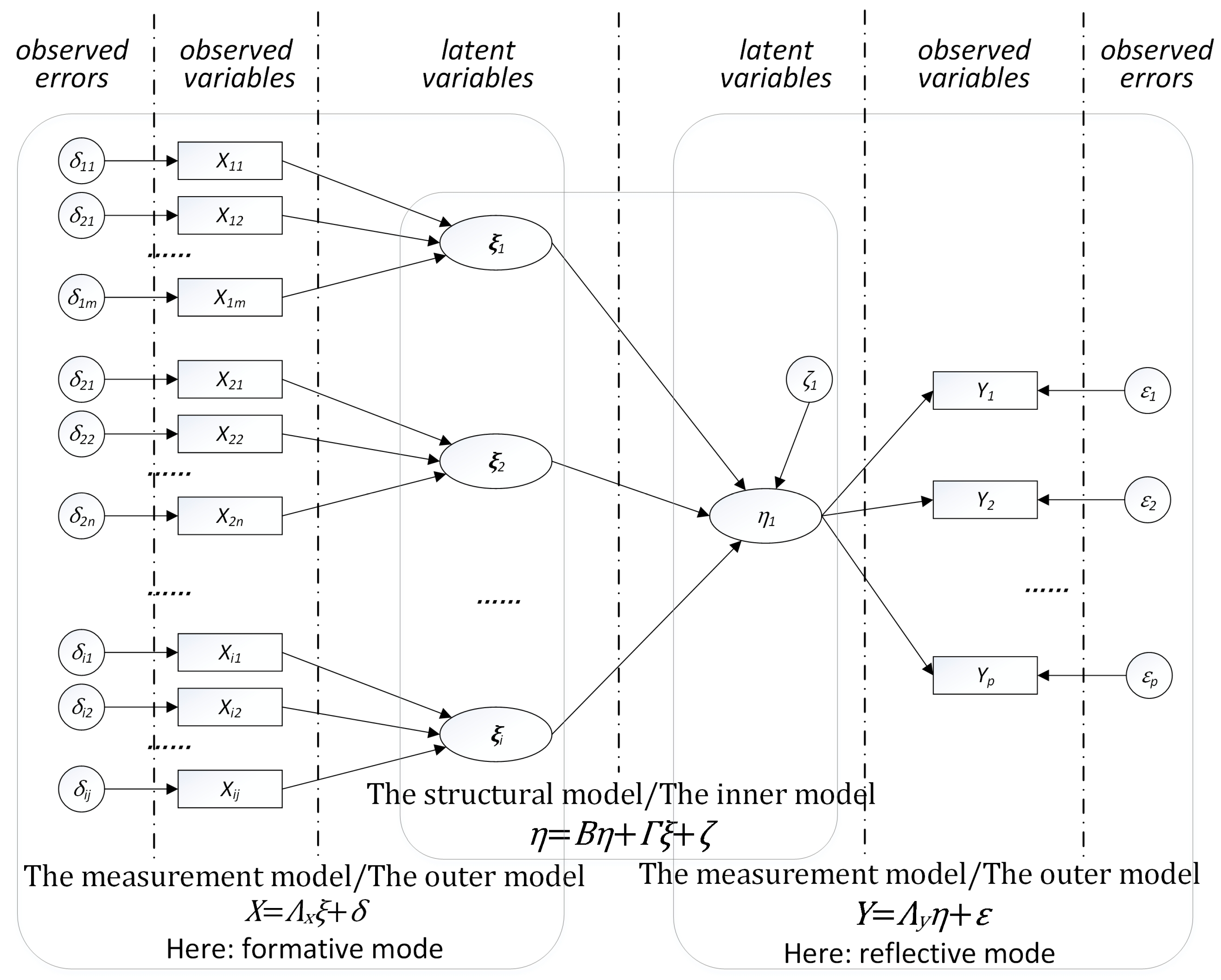
3.1. Rationale for SEM
3.2. Model Building for Urban Competitiveness Measurement
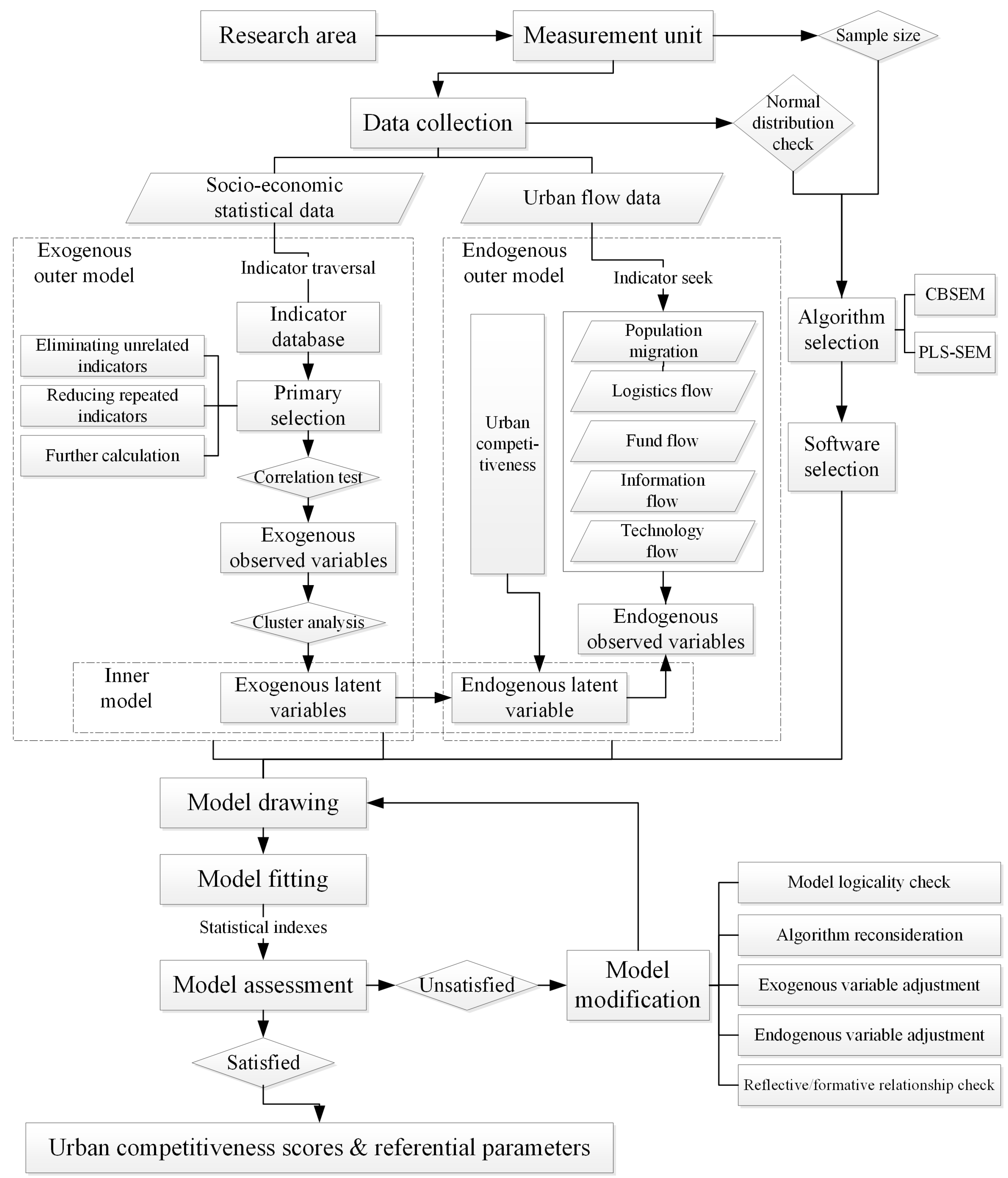
3.2.1. Algorithm Selection
3.2.2. Model Building
Model Design
Exogenous Outer Model
- Step 1
- 2011 Urban Statistical Yearbook of China offers urban attribute indicators for our research. We collected 123 indicators for municipal districts of cities by traversing the yearbook. This is the primary indicator database for our research.
- Step 2
- We considered the indicators collected one by one and made our primary selection. Indicators that obviously have nothing to do with urban competitiveness, such as number of primary schools and middle-school student enrollment, should be eliminated. Some indicators need to be calculated further as per capita data or percentiles to reflect urban competitiveness better, such as changing registered unemployed people to the unemployment rate. Moreover, when more than one indicator reflects the same or similar meaning, such as population at year-end and average population, they should be reduced to one. In total, 113 indicators were left in our research after primary selection.
- Step 3
- We reselected indicators according to correlation test. This test was processed in SPSS after data standardization. Significant correlation indicators should be eliminated. There were 20 indicators left after reselection, which were defined as observed variables in our exogenous outer model.
- Step 4
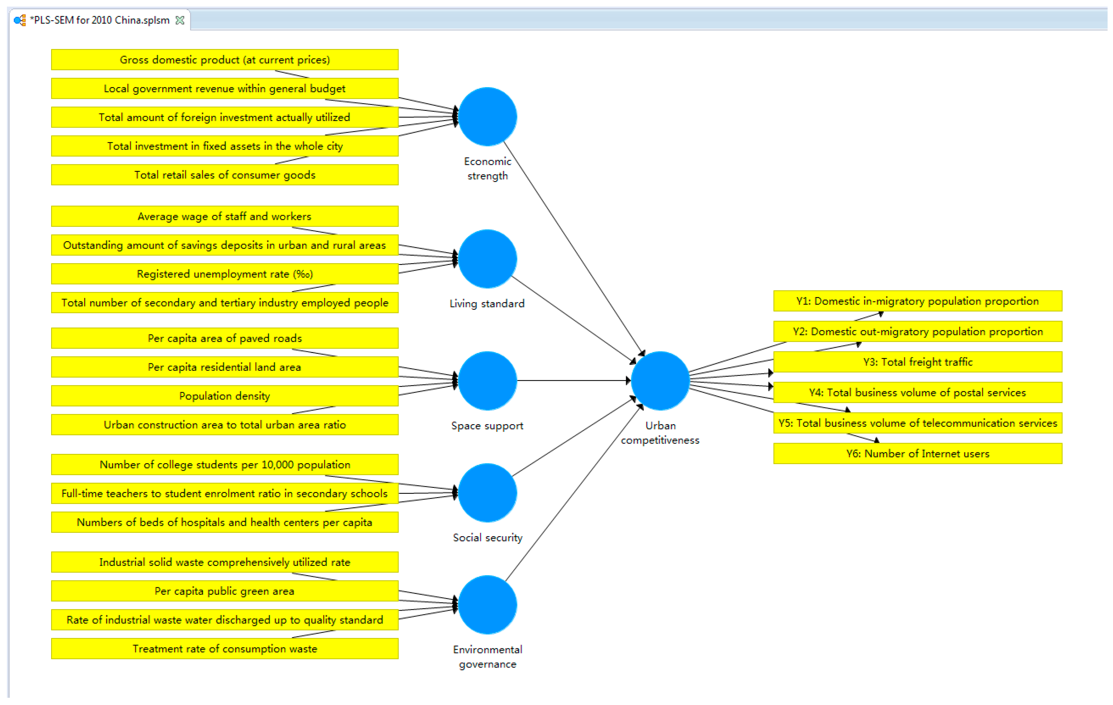
- We clustered the reselected indicators through principal component analysis. This can also be achieved in SPSS. The cluster results should be checked: indicators reflecting the same aspects of urban characteristics or urban competitiveness should be clustered into one dimension; the indicator number of each dimension should meet the basic requirement of SEM. Necessary replacement or adjustment on reselected indicators can be helpful for cluster outcome. Dimensions obtained from the analysis should present a certain perspective of urban characteristics corresponding to several observed indicators, thereby defining latent variables of the exogenous outer model. We identified five major dimensions of the 20 indicators, which are expressions of economic strength, living standard, space support, social security, and environmental governance.
Endogenous Outer Model
Inner Model
3.2.3. Model Fitting and Assessment
3.2.4. Model Modification
4. Results and Discussion
4.1. Urban Competitiveness Distribution Characteristics in 2010 China
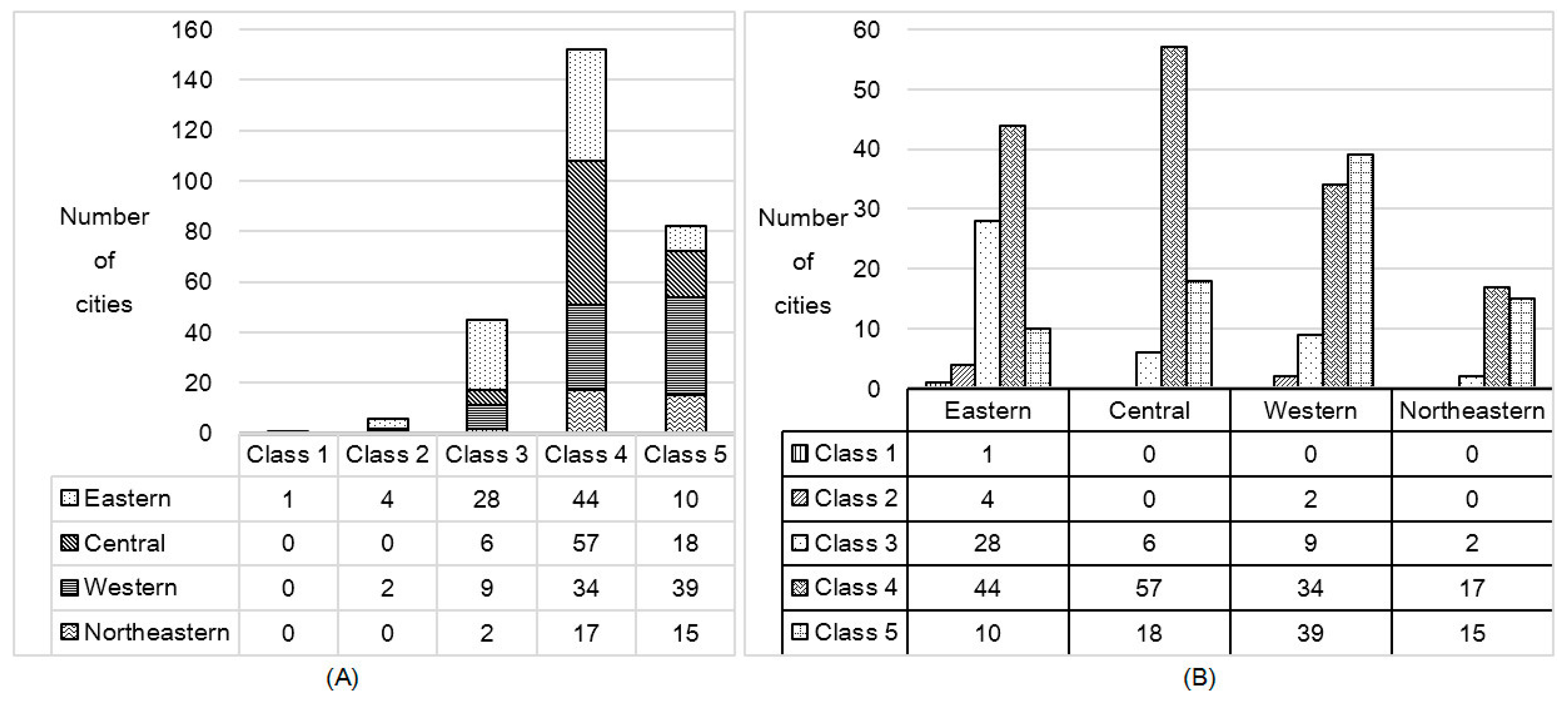
4.1.1. Quantitative Characteristic
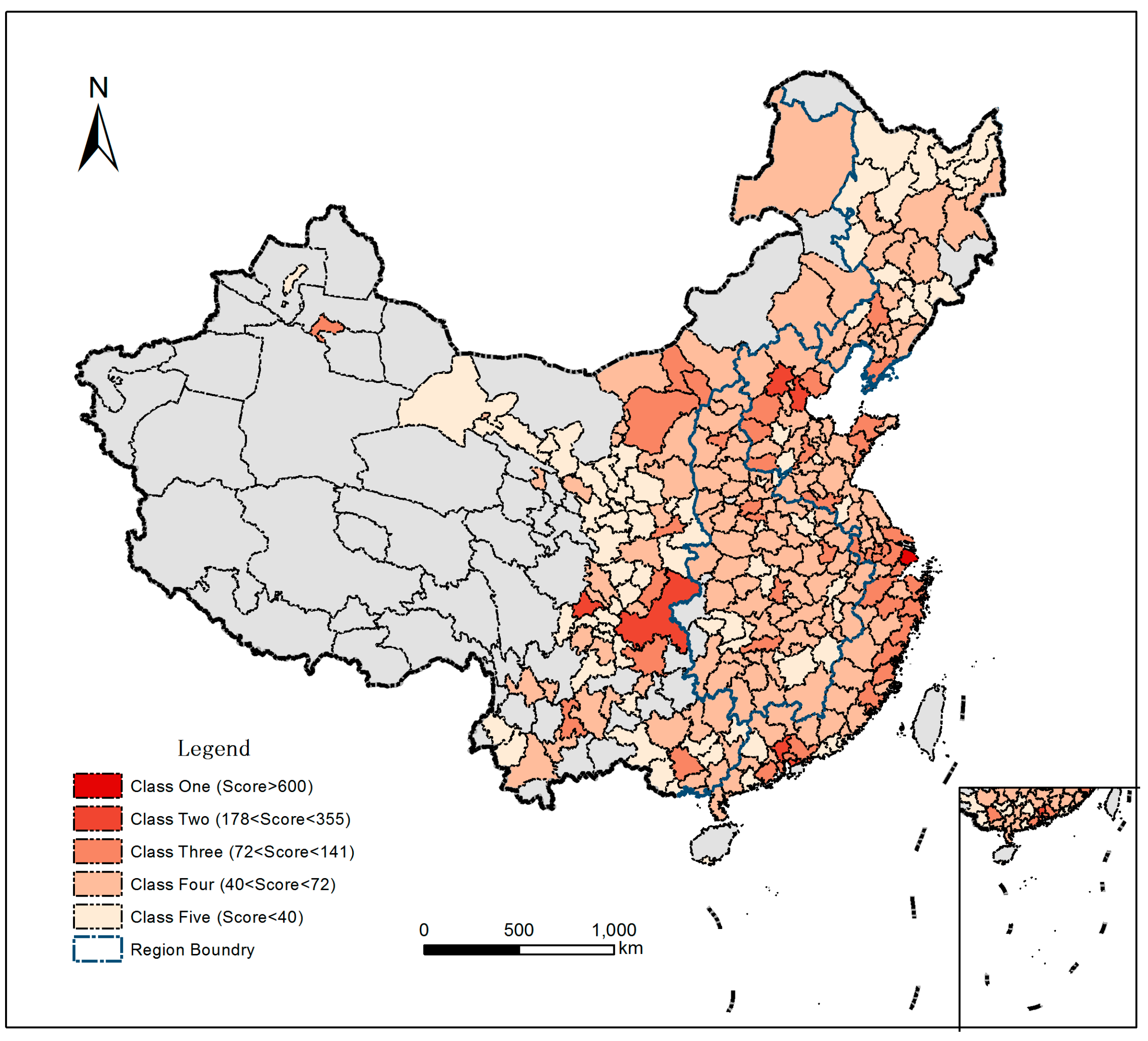
4.1.2. Spatial Distribution Characteristic
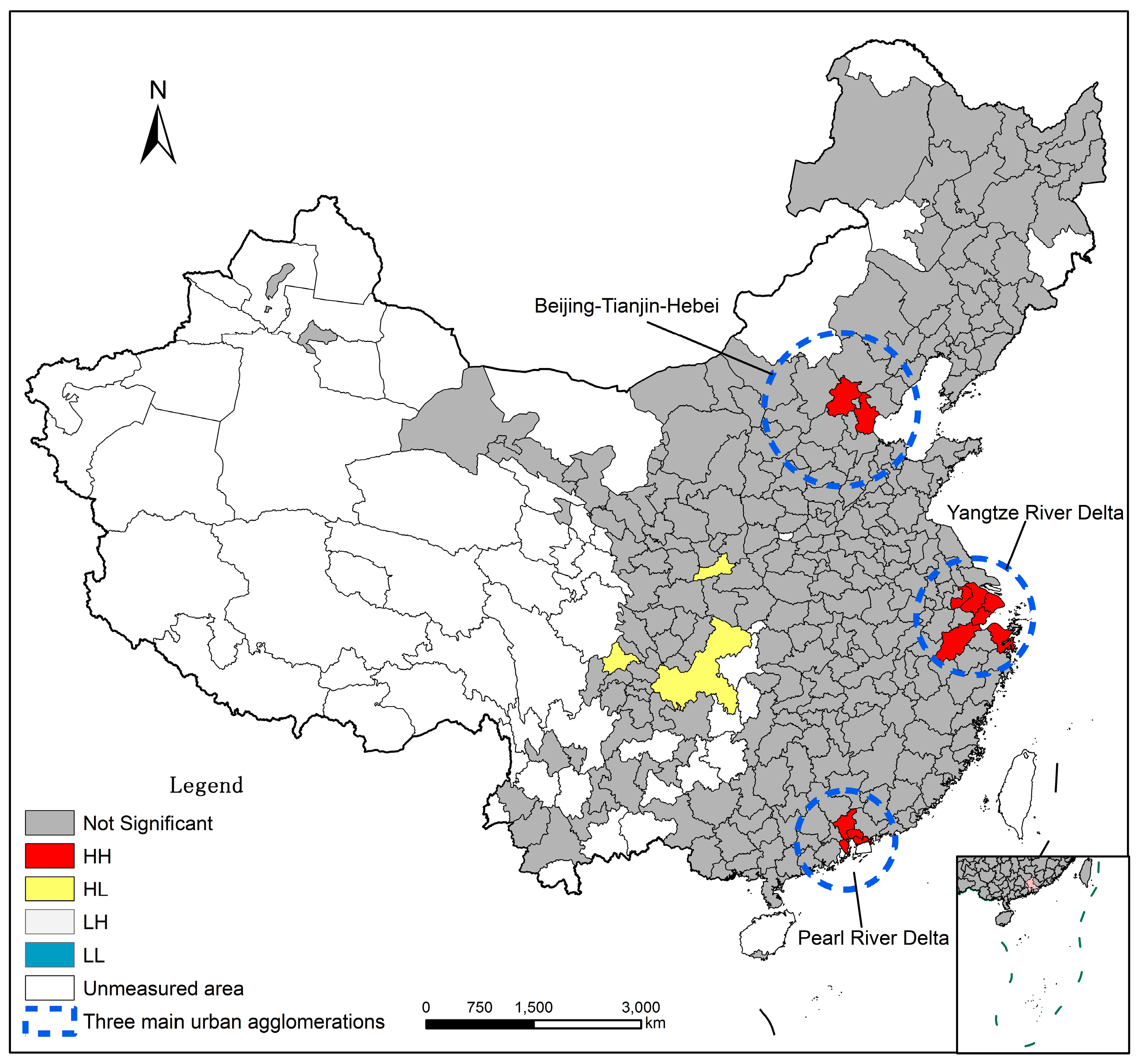
4.1.3. Spatial Correlation Characteristic
4.2. Influencing Factors of Urban Competitiveness in China in 2010
4.2.1 Correlation between Urban Attributes and Urban Competitiveness in China in 2010
4.2.2. Correlation between Urban Competitiveness and Urban Flows in China in 2010
5. Discussion on PLS-SEM Approach
5.1. Reliability of Results
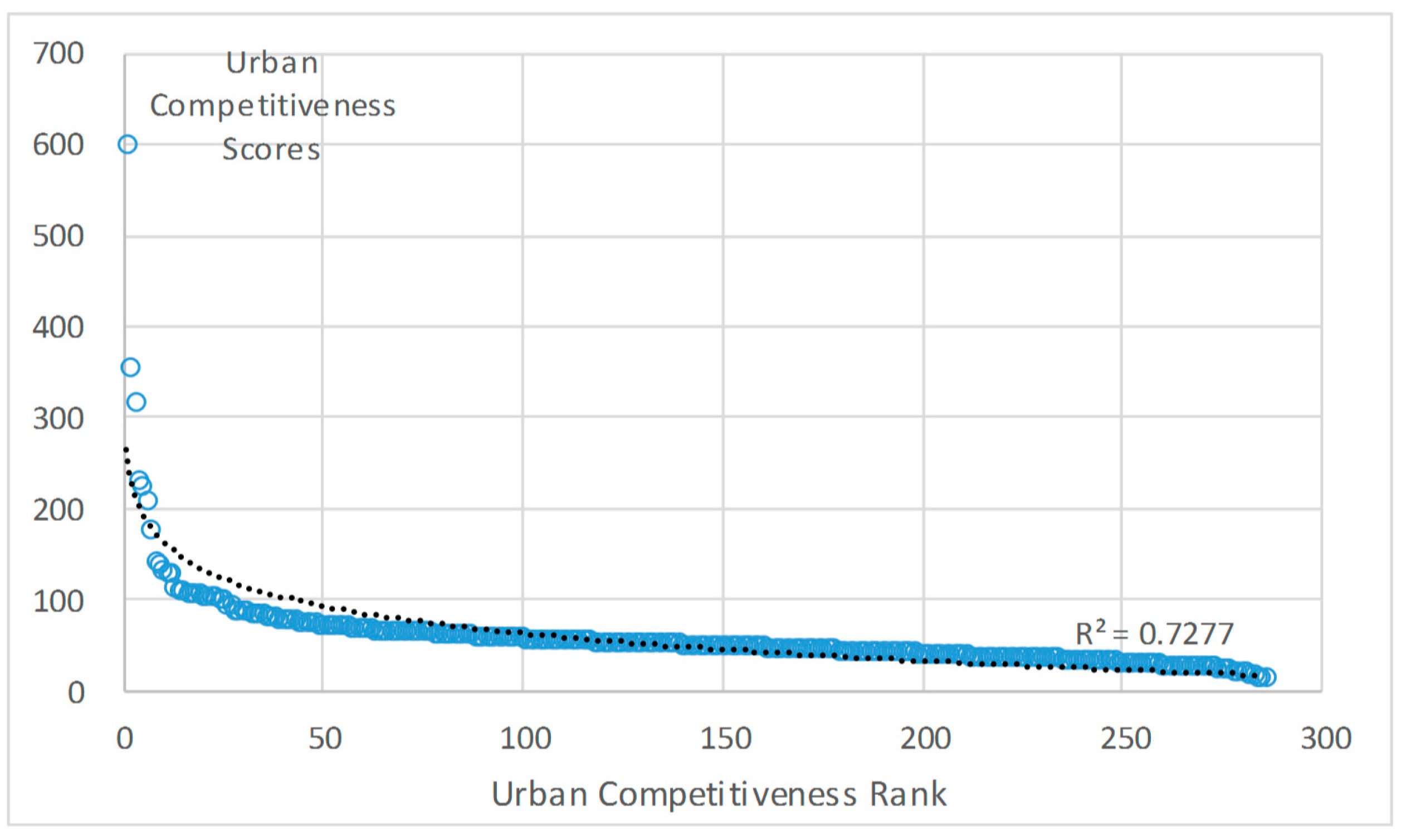
5.1.1. Result Testing Based on Rank-Size Rule
5.1.2. Result Comparison with Other Approaches
5.2. Theoretical Reliability
5.3. Statistical Reliability
6. Conclusions
Acknowledgments
Author Contributions
Conflicts of Interest
References
- Sáez, L.; Periáñez, I. Benchmarking urban competitiveness in europe to attract investment. Cities 2015, 48, 76–85. [Google Scholar] [CrossRef]
- Shen, J.; Yang, X. Analyzing urban competitiveness changes in major chinese cities 1995–2008. Appl. Spat. Anal. Policy 2014, 7, 361–379. [Google Scholar] [CrossRef]
- Jiang, Y.; Shen, J. Weighting for what? A comparison of two weighting methods for measuring urban competitiveness. Habitat Int. 2013, 38, 167–174. [Google Scholar] [CrossRef]
- Ni, P.F.; Kresl, P.; Li, X.J. China urban competitiveness in industrialization: Based on the panel data of 25 cities in china from 1990 to 2009. Urban Stud. 2014, 51, 2787–2805. [Google Scholar] [CrossRef]
- Reed, H.C. The Pre-Eminence of International Financial Centres; Praeger: New York, NY, USA, 1981. [Google Scholar]
- Ding, L.; Shao, Z.F.; Zhang, H.C.; Xu, C.; Wu, D.W. A comprehensive evaluation of urban sustainable development in china based on the topsis-entropy method. Sustainability 2016, 8, 23. [Google Scholar] [CrossRef]
- Friedmann, J. The world city hypothesis. Dev. Change 1986, 17, 69–83. [Google Scholar] [CrossRef]
- Sassen, S. The Global City: New York, London, Tokyo; Princeton University Press: Princeton, NJ, USA, 1991. [Google Scholar]
- Pal, A. The connected city: How networks are shaping the modern metropolis. Int. J. Urban Reg. Res. 2014, 38, 2. [Google Scholar]
- Beaverstock, J.V.; Doel, M.A.; Hubbard, P.J.; Taylor, P.J. Attending to the world: Competition, cooperation and connectivity in the world city network. Glob. Netw. 2002, 2, 111–132. [Google Scholar] [CrossRef]
- Burger, M.J.; van Oort, F.G.; Wall, R.S.; Thissen, M.J.P.M. Analysing the competitive advantage of cities in the dutch randstad by urban market overlap. In Metropolitan Regions: Knowledge Infrastructures of the Global Economy; Klaesson, J., Johansson, B., Karlsson, C., Eds.; Springer: Berlin, Germany, 2013; pp. 375–391. [Google Scholar]
- Gedikli, B. Interurban Competition within the Circumstances Created by Global Capitalism; GaWC Research Network: Leicestershire, UK, 2001. [Google Scholar]
- Benton-Short, L.; Price, M.D.; Friedman, S. Globalization from below: The ranking of global immigrant cities. Int. J. Urban Reg. Res. 2005, 29, 945–959. [Google Scholar] [CrossRef]
- Mahutga, M.C.; Ma, X.; Smith, D.A.; Timberlake, M. Economic globalisation and the structure of the world city system: The case of airline passenger data. Urban Stud. 2010, 47, 1925–1947. [Google Scholar] [CrossRef]
- Alderson, A.S.; Beckfield, J.; Sprague-Jones, J. Intercity relations and globalisation: The evolution of the global urban hierarchy, 1981–2007. Urban Stud. 2010, 47, 1899–1923. [Google Scholar] [CrossRef]
- Bowen, J. Network change, deregulation, and access in the global airline industry. Econ. Geogr. 2002, 78, 425–439. [Google Scholar] [CrossRef]
- Martin, R. Keys to the city: How economics, institutions, social interaction, and politics shape development. Econ. Geogr. 2014, 90, 341–344. [Google Scholar] [CrossRef]
- Jöreskog, K.G. A general method for analysis of covariance structures. Biometrika 1970, 57, 239–251. [Google Scholar] [CrossRef]
- Population Census Office under the State Council; Department of Population and Employment Statistics National Bureau of Statistics. Tabulation on the 2010 Population Census of the People's Republic of China by County; China Statistics Press: Beijing, China, 2011.
- City Socio-economic Survey Office of National Bureau of Statistics. 2011 Urban Statistical Yearbook of China; China Statistics Press: Beijing, China, 2012.
- Gefen, D.; Straub, D.W.; Boudreau, M.-C. Structural equation modelling and regression: Guidelines for research practice. Commun. Assoc. Inf. Syst. 2000, 4, 1–78. [Google Scholar]
- Henseler, J.; Ringle, C.M.; Sinkovics, R.R. The use of partial least squares path modeling in international marketing. Adv. Int. Mark. 2009, 20, 277–319. [Google Scholar]
- Wold, H. Soft modelling: The basic design and some extensions. In System under Indirect Observation: Causality, Structure, Prediction, Part II; Acedemic Press: Cambridge, MA, USA, 1982; pp. 36–37. [Google Scholar]
- Wold, H. Partial least squares. In Encyclopedia of Statistical Sciences; John Wiley & Sons, Inc.: Somerset, NJ, USA, 2004. [Google Scholar]
- Jöreskog, K.G.; Wold, H. The ml and pls techniques for modelling with latent variables: Historical and comparative aspects. In Systems under Indirect Observation; North-Holland: Amsterdam, The Netherlands, 1982; Volume 1, pp. 263–270. [Google Scholar]
- Wold, H. Model construction and evaluation when theoretical knowledge is scarce. In Evaluation Economic Models; Academic Press: Cambridge, MA, USA, 1980; pp. 47–74. [Google Scholar]
- Tenenhaus, M.; Vinzi, V.E.; Chatelin, Y.-M.; Lauro, C. Pls path modeling. Comput. Stat. Data Anal. 2005, 48, 159–205. [Google Scholar] [CrossRef]
- Lohmöller, J.-B. Latent Variable Path Modeling with Partial Least Squares; Physica-Verlag HD: Heidelberg, Germany, 1989. [Google Scholar]
- Ringle, C.M.; Wende, S.; Becker, J.-M. Smartpls 3; SmartPLS: Hamburg, Germany, 2005; Available online: http://www.smartpls.de (accessed on 26 July 2014).
- Cronbach, L. Coefficient alpha and the internal structure of tests. Psychom 1951, 16, 297–334. [Google Scholar] [CrossRef]
- Nunnally, J. Psychometric Theory; McGraw-Hill: New York, NY, USA, 1967. [Google Scholar]
- Werts, C.E.; Linn, R.L.; Jöreskog, K.G. Intraclass reliability estimates: Testing structural assumptions. Educ. Psychol. Meas. 1974, 34, 25–33. [Google Scholar] [CrossRef]
- Fornell, C.; Larcker, D.F. Structural equation models with unobservable variables and measurement error: Algebra and statistics. J. Mark. Res. 1981, 18, 382–388. [Google Scholar] [CrossRef]
- Chin, W.W.; Marcoulides, G.A.; Press, P. The partial least squares approach to structural equation modeling. In Modern Methods for Business Research; Lawrence Erlbaum Associates Publishers: Mahwah, NJ, USA, 1998; p. 323. [Google Scholar]
- Zhao, F. Research of Customer Satisfaction Measurement Based on PLS Path Modeling. Ph.D. Thesis, Tianjin University, Tianjin, China, 2010. [Google Scholar]
- Rosen, K.T.; Resnick, M. The size distribution of cities: An examination of the pareto law and primacy. J. Urban Econ. 1980, 8, 165–186. [Google Scholar] [CrossRef]
- Singer, H.W. The “courbe des populations”. A parallel to pareto’s law. Econ. J. 1936, 46, 254–263. [Google Scholar] [CrossRef]
- Dai, H. Study on the type of urban scale distribution and its developing mechanism in China. Hum. Geogr. 2001, 16, 40–43,57. [Google Scholar]
- Li, Z.; Yang, Y. Hierarchy flatening or enlarging: Research on the changing trend of chinese urban hiearachy based on gdp size distribution. Plan. Stud. 2010, 34, 28–32. [Google Scholar]
- Tan, M.; Lv, C. Distrubution of china city size expressed by urban built-up area. Acta Geogr. Sin. 2003, 58, 285–293. [Google Scholar]


| Assessed Part | Context | Criterion | Description | Suggest Extent | Model Fitting Result | |||
|---|---|---|---|---|---|---|---|---|
| Reflective outer model | Internal consistency reliability | Cronbach’s α [30] | Assume that all indicators are equally reliable, and then estimate reliability based on the indicator inter-correlations. | >0.7 [31] | Cronbach’s α = 0.74, fits well. | |||
| Composite reliability ρc [32] | As above, but taking differences between indicator loadings into account. | >0 [31] | Composite reliability ρc = 0.84, fits well. | |||||
| Indicator reliability | Absolute standard outer loadings | A latent variable should explain a substantial part of each indicator’s variance (usually at least 50%). | >0.7 () | Variables | Y1 | Y2 | Y3 | |
| Loading | 0.582 | −0.194 | 0.732 | |||||
| Fitness | Below | Below | Fit | |||||
| Variables | Y4 | Y5 | Y6 | |||||
| Loading | 0.917 | 0.906 | 0.816 | |||||
| Fitness | Fit | Fit | Fit | |||||
| Convergent validity | Average variance extracted (AVE) | Measuring how much a latent variable is able to explain the variance of its indicators on average. | >0.5 [33] | AVE = 0.54, fits well. | ||||
| Discriminant validity | Fornell–Larcker criterion or cross-loadings | Two conceptually different concepts should exhibit sufficient difference. | — | Not necessary for this part because there is only one latent variable in our model. | ||||
| Formative outer model | Nomological validity | Hypotheses check | Assessing whether the formative index behaves within a net of hypotheses as expected, and whether those relationships between the formative index and other constructs in the path model that are sufficiently referred to in prior research are strong and significant. | Compare gradually | Relationship | Loading | Fitness | |
| ζ1→η | 0.74 | Fit | ||||||
| ζ2→η | 0.17 | Fit | ||||||
| ζ3→η | 0.11 | Fit | ||||||
| ζ4→η | 0.07 | Fit | ||||||
| ζ5→η | −0.03 | Fit | ||||||
| External validity | 1-Var (v) | Measuring how much of the construct is not captured by any indicator by means of regressing the formative index on a reflective measure of the same construct. | >0.8 [22] | Fits well. | ||||
| Multicollinearity | Variance inflation factor (VIF) | Assessing the degree of multicollinearity among manifest variables in a formative block. | <10 [22] | Each fits well. | ||||
| Inner model | Determination coefficient | R2 | Evaluating the fitting degree of the endogenous latent variables. | >0.67 [34] | R2 = 0.89, fits well. | |||
| Bootstrapping | Weights and path coefficients | Students’ T-test | Revealing the significance of path model relationships by creating a large, prespecified number of bootstrap samples. | Student’s t-distribution table | Each fits well. | |||
| Class | City Number | Accumulated Number | Score Extent |
|---|---|---|---|
| 1 | 1 | 1 | 601.22 |
| 2 | 6 | 7 | 178.34–354.12 |
| 3 | 45 | 52 | 72.56–140.50 |
| 4 | 152 | 204 | 40.71–71.54 |
| 5 | 82 | 286 | 13.35–39.88 |
| Class | Rank | City | Score | Rank | City | Score |
|---|---|---|---|---|---|---|
| 1 | 1 | Shanghai | 601.22 | |||
| 2 | 2 | Beijing | 354.12 | 5 | Tianjin | 224.45 |
| 3 | Shenzhen | 316.78 | 6 | Guangzhou | 209.74 | |
| 4 | Chongqing | 231.57 | 7 | Chengdu | 178.34 |
| Variables | Correlation | Path Coefficient | |
|---|---|---|---|
| ζ1→η | Economic strength → Urban competitiveness | Positive | 0.71 |
| ζ2→η | Living standard → Urban competitiveness | Positive | 0.21 |
| ζ3→η | Space support → Urban competitiveness | Positive | 0.06 |
| ζ4→η | Social security → Urban competitiveness | Positive | 0.06 |
| ζ5→η | Environmental governance → Urban competitiveness | Negative | −0.02 |
| Urban Flow | Variables | Loading | |
|---|---|---|---|
| Population migration | Y1 | Overall population migratory proportion | 0.65 |
| Logistic flow | Y2 | Total freight traffic | 0.74 |
| Y3 | Total business volume of postal services | 0.93 | |
| Information flow | Y4 | Total business volume of telecommunication services | 0.91 |
| Y5 | Number of Internet users | 0.82 | |
| Correlation Coefficient | PLS-SEM Measurement | Competitiv-Eness in Blue Book | Average Population | GDP | Area of Built Urban District |
|---|---|---|---|---|---|
| PLS-SEM measurement | 1 | ||||
| Competitiveness in Blue Book | 0.645 ** | 1 | |||
| Average population | 0.779 ** | 0.572 ** | 1 | ||
| GDP | 0.913 ** | 0.687 ** | 0.853 ** | 1 | |
| Area of built urban district | 0.825 ** | 0.699 ** | 0.882 ** | 0.913 ** | 1 |
© 2017 by the authors. Licensee MDPI, Basel, Switzerland. This article is an open access article distributed under the terms and conditions of the Creative Commons Attribution (CC BY) license (http://creativecommons.org/licenses/by/4.0/).
Share and Cite
Yuan, Z.; Zheng, X.; Zhang, L.; Zhao, G. Urban Competitiveness Measurement of Chinese Cities Based on a Structural Equation Model. Sustainability 2017, 9, 666. https://doi.org/10.3390/su9040666
Yuan Z, Zheng X, Zhang L, Zhao G. Urban Competitiveness Measurement of Chinese Cities Based on a Structural Equation Model. Sustainability. 2017; 9(4):666. https://doi.org/10.3390/su9040666
Chicago/Turabian StyleYuan, Zhiyuan, Xinqi Zheng, Lulu Zhang, and Guoliang Zhao. 2017. "Urban Competitiveness Measurement of Chinese Cities Based on a Structural Equation Model" Sustainability 9, no. 4: 666. https://doi.org/10.3390/su9040666
APA StyleYuan, Z., Zheng, X., Zhang, L., & Zhao, G. (2017). Urban Competitiveness Measurement of Chinese Cities Based on a Structural Equation Model. Sustainability, 9(4), 666. https://doi.org/10.3390/su9040666