Multi-Objective Spatial Optimization: Sustainable Land Use Allocation at Sub-Regional Scale


Abstract
:1. Introduction
2. Materials and Methods
2.1. Problem Formulation
2.1.1. Income Maximization
2.1.2. Minimizing Negative Pressures on the Environment
2.1.3. Minimizing Food Deficit
2.2. Restrictions
- -
- Total surface per land use u, varies between the fixed lower and upper limits Pu low and Pu up, respectively.
- -
- The sum of all land uses is the whole grid cell area
- -
- Land uses are allocated according to territorial aptitude. It is assumed that a cell in the territory may be suitable for several uses at once. Therefore, when the territory is considered as a topologic space, there is a viable subset of cells for every use u, Su.
- -
- The sum of cells ij with use u is always lower than its viable subset
- -
- Viable subsets are contained in the cell grid
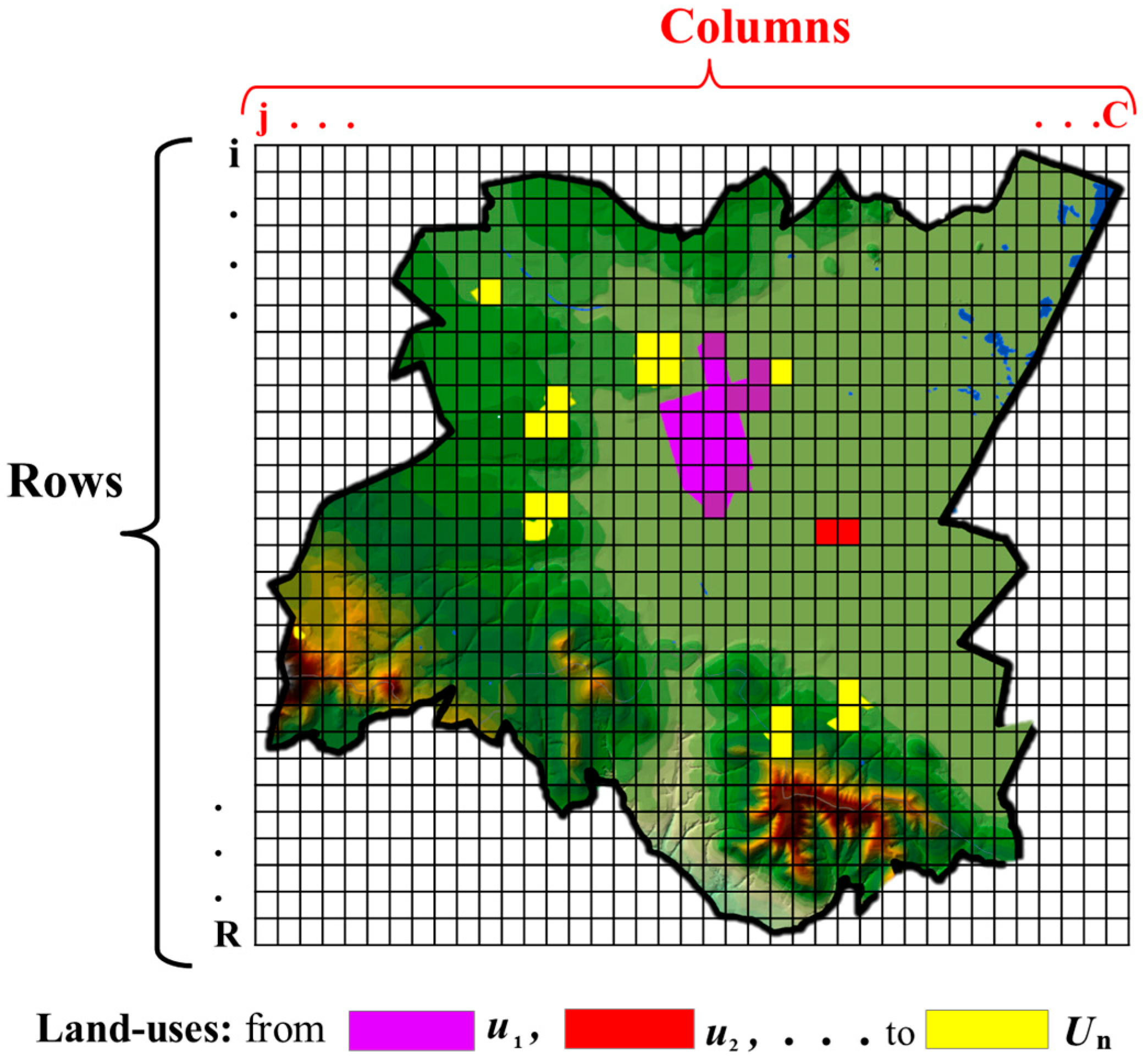
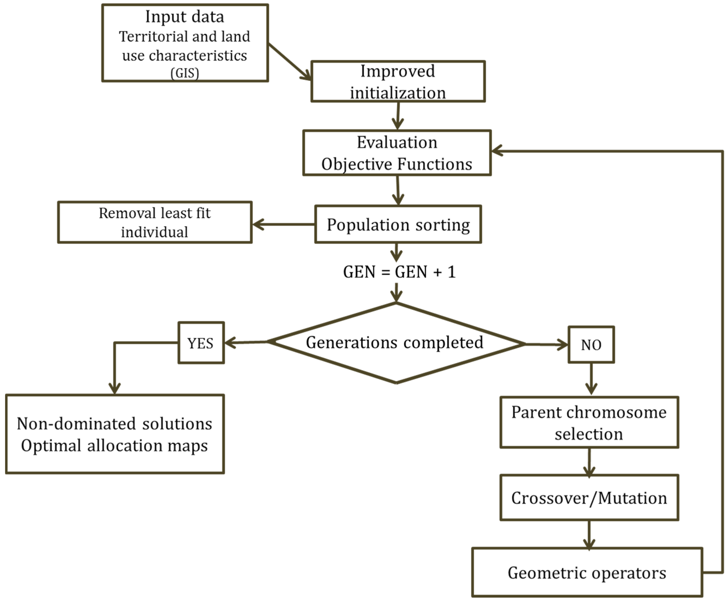
2.3. Model for Sustainable Land Use Allocation: MAUSS
2.3.1. Chromosome Representation
2.3.2. Initialization
- (a)
- Random seed cells and their subsequent agglomeration must be allocated in an empty cell within a valid land use subset.
- (b)
- The sum of cells per land use must not exceed the pre-fixed area. Each land use can be allocated in one or several agglomerations depending on the seed randomization parameter.
- (c)
- Only one land use type can be allocated in a cell
- Random selection of land use allocation order.
- Random selection of seed cells for initiating the agglomeration by allocating the current land use in its eight neighbor cells (3 × 3 cell window). Adjacent cells are then identified (5 × 5 cell window) to act as new seeds until the maximum area per use is reached. All individual cells must accomplish the above considerations.
- Once the current land use cells are completely allocated, the process continues with the next random land use until the chromosome allocates all land uses.
- The initialization process iterates until the initial set of chromosomes (population) is completed.
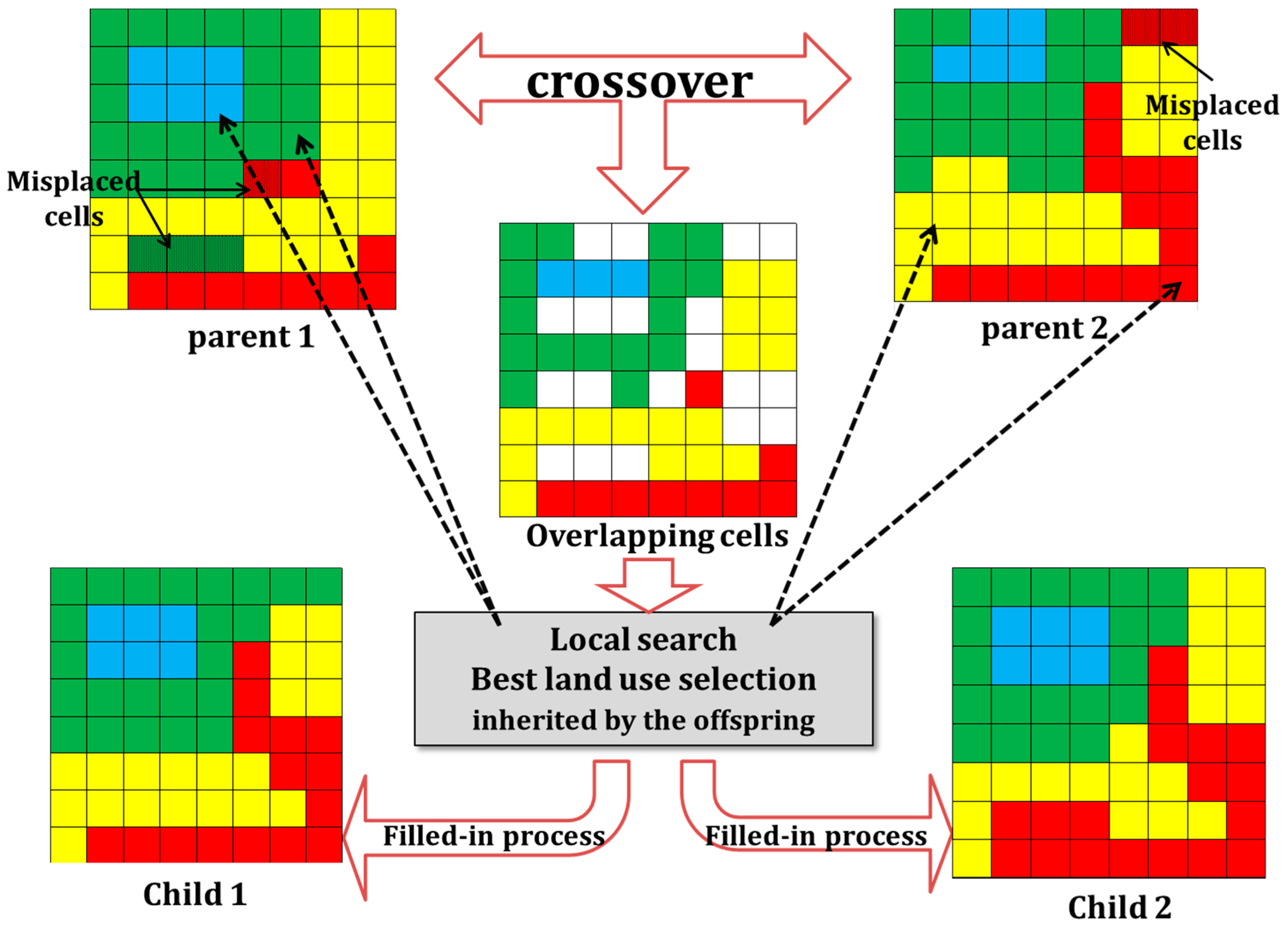
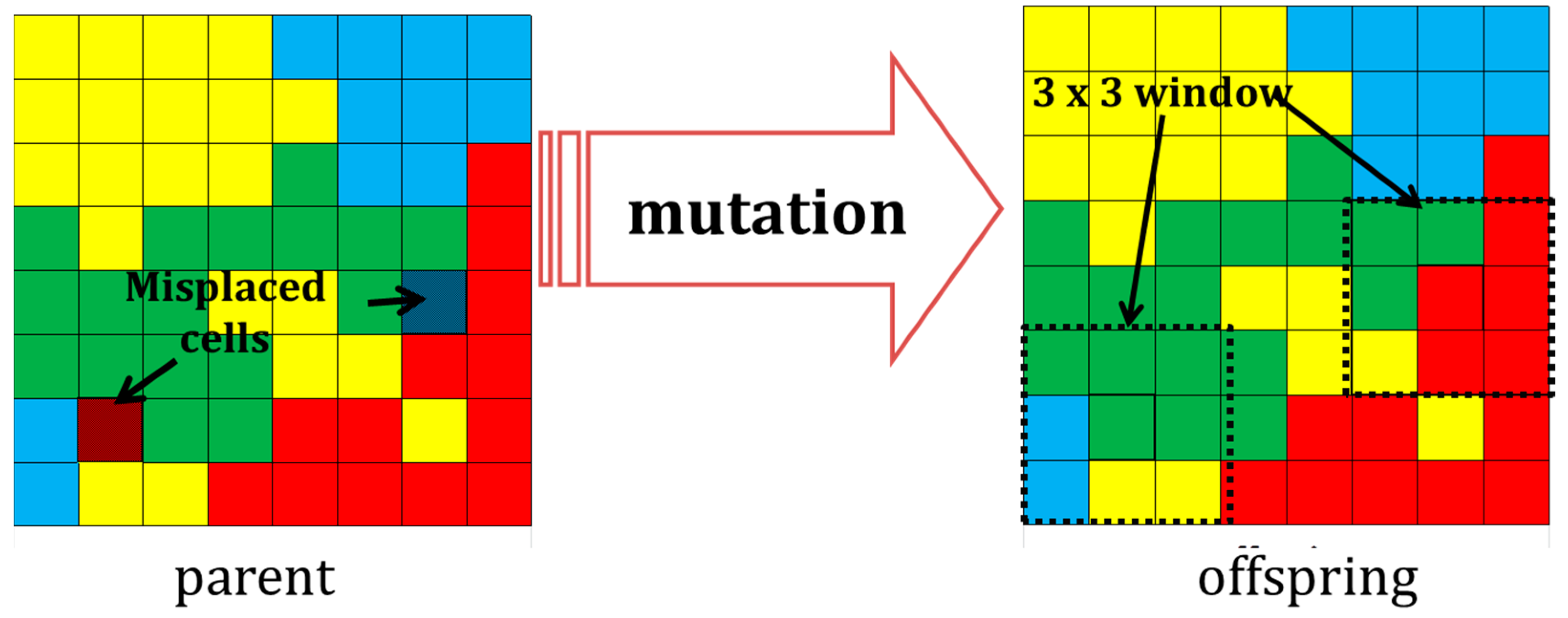
2.3.3. Model Operators
- (1)
- Overlapping stage: Cells of parent one and parent two in whose positions land use type is equal (overlapped cells) are inherited by child one and child two provided they are located within their valid subsets. Matching cells containing different land uses remain empty.
- (2)
- Local search stage: To fill empty cells, a local search is applied in this work for each land use type by a similar procedure to that proposed by Datta et al. [5]. The objective functions of the model are evaluated in each parent per land use at a time into one minimization function OU (Equation (11)). In contrast to the authors above, the result is not weighted but compared with both parents. The land use with the minimum value is then allocated in the empty cells of child 1 and child 2 alternatively, provided that the above restrictions are accomplished (Equations (6)–(10)). Therefore, the offspring inherits the best land use allocations obtained by the local search and improves global chromosome evaluation.where M is the number of objective functions of the model from j to M; is the value of current land use from i to U evaluated at the jth objective for the (x) parent (parent 1 or parent 2); and and are the maximum and minimum values obtained from the initial population set evaluated for the ith (current) land use U at the jth objective function.
- (3)
- Filled-in stage: The remaining empty cells, which are those outside their valid subset (misplaced), go through a filled-in process similar to the initialization process above. Specifically, the process starts with the random allocation of seed cells (according to the randomization parameter) per deficit land use at least until the lower surface limit for the current land use is reached. This process iterates in descending order beginning from the highest land use deficit (that could be 100 percent). If there is more than one absent land use in the offspring, the iteration process starts with the land use of the smallest extension, provided that restrictions are being accomplished.
- (1)
- Identifies cells with misplaced land uses.
- (2)
- In a 3 × 3 analysis window, misplaced cells take the most frequent land use in the window if they are exclusively within their valid subsets.
- (1)
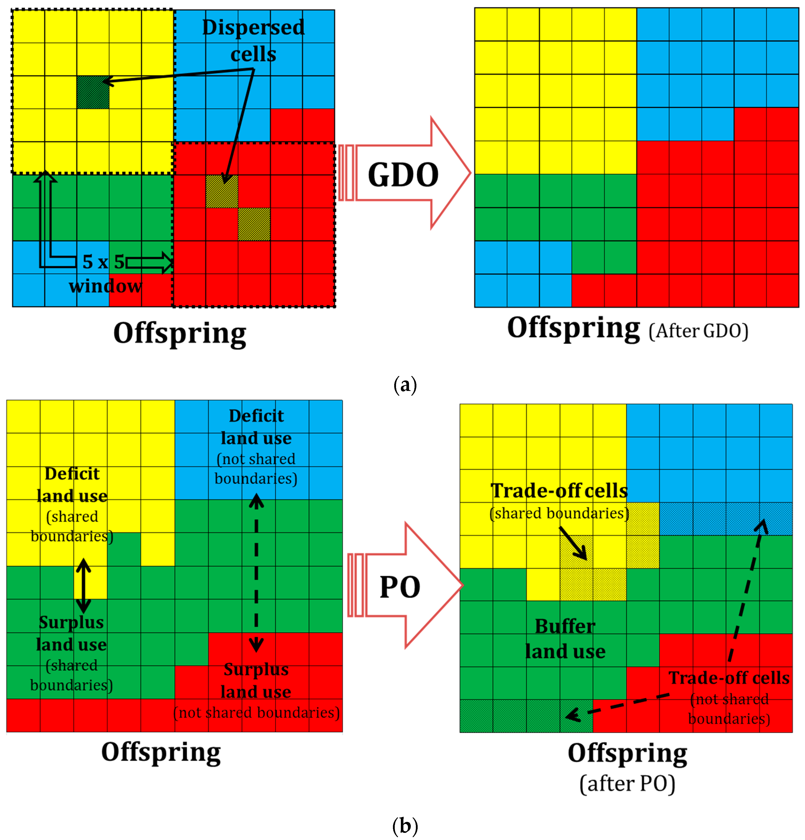
- The geographic dispersion operator (GDO) was designed to enhance the compactness of patches. The GDO identifies land use cells allocated either within or outside their feasible subset in a 5 × 5-analysis cell window spread (Figure 4a). Once identified, they turn into the most frequent land use of the neighboring cells. Geographic dispersion must be defined for each implementation of the model because it depends on both geographic extent and cell size, and is related to the specific spatial optimization targets and the available local cartography. In this work, dispersion is understood in the analysis window as one or two maximum adjacent cells whose land use type differs from the remaining neighboring cells. The process iterates until there are no more spread cells in the grid.
- (2)
- The proportion operator (PO) performs by land-use pairs at a time and controls the number of cells required per land use through a patch boundary analysis. Firstly, the operator identifies unbalanced (deficit or surplus) land uses. Each unbalanced land use type can be allocated in one or several cell patches. The land uses with the highest deficit and highest surplus are then chosen. Secondly, the boundary analysis indicates if both uses are neighbors at least in one patch or not. In the first case, the trade-off is immediate only in cells within the constraints; hence the deficit/surplus could be balanced or diminished, but enables the operator to choose a second pair of land uses of unbalanced size using the same criterion as above. This process iterates until all land use sizes are compensated or until there are no neighbors between the remaining unbalanced land uses. In that case, a different land use patch that shares boundaries with a deficit patch enables proportioning by ceding cells which are transformed into the deficit land use type and later compensated by the surplus land use. This operator iterates in two or more patches until map land uses proportion (within the upper and lower limits of pre-fixed areas) is reached, provided that the spatial restrictions are fulfilled (Figure 5b).
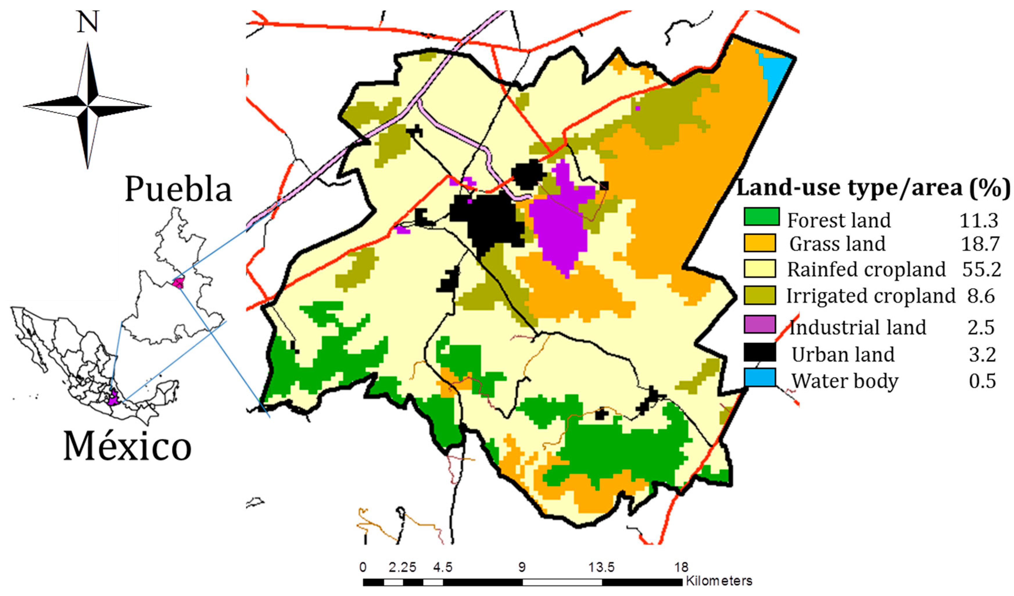
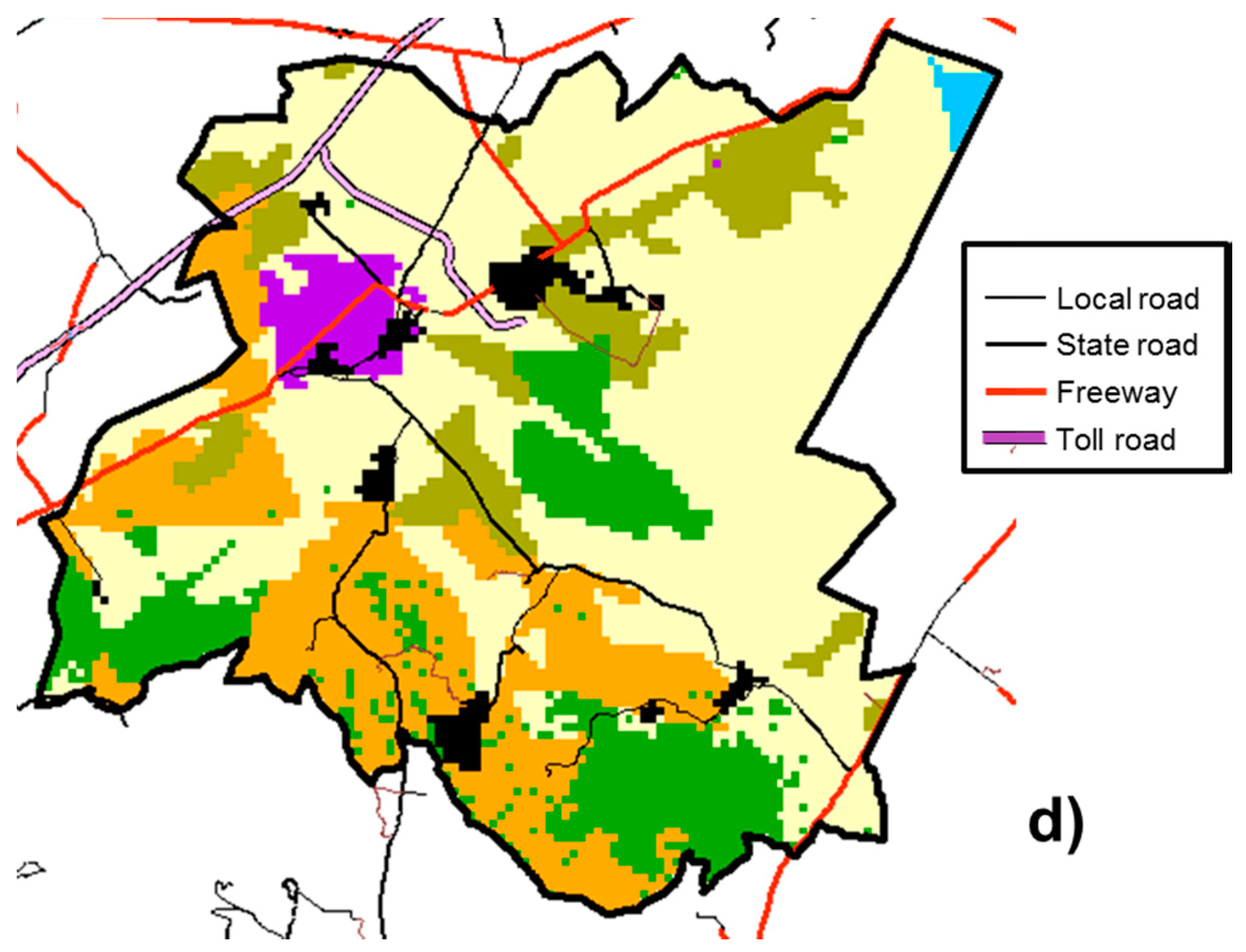
2.4. Case Study. Application of MAUSS to the Plains of San Juan
Study Area Description
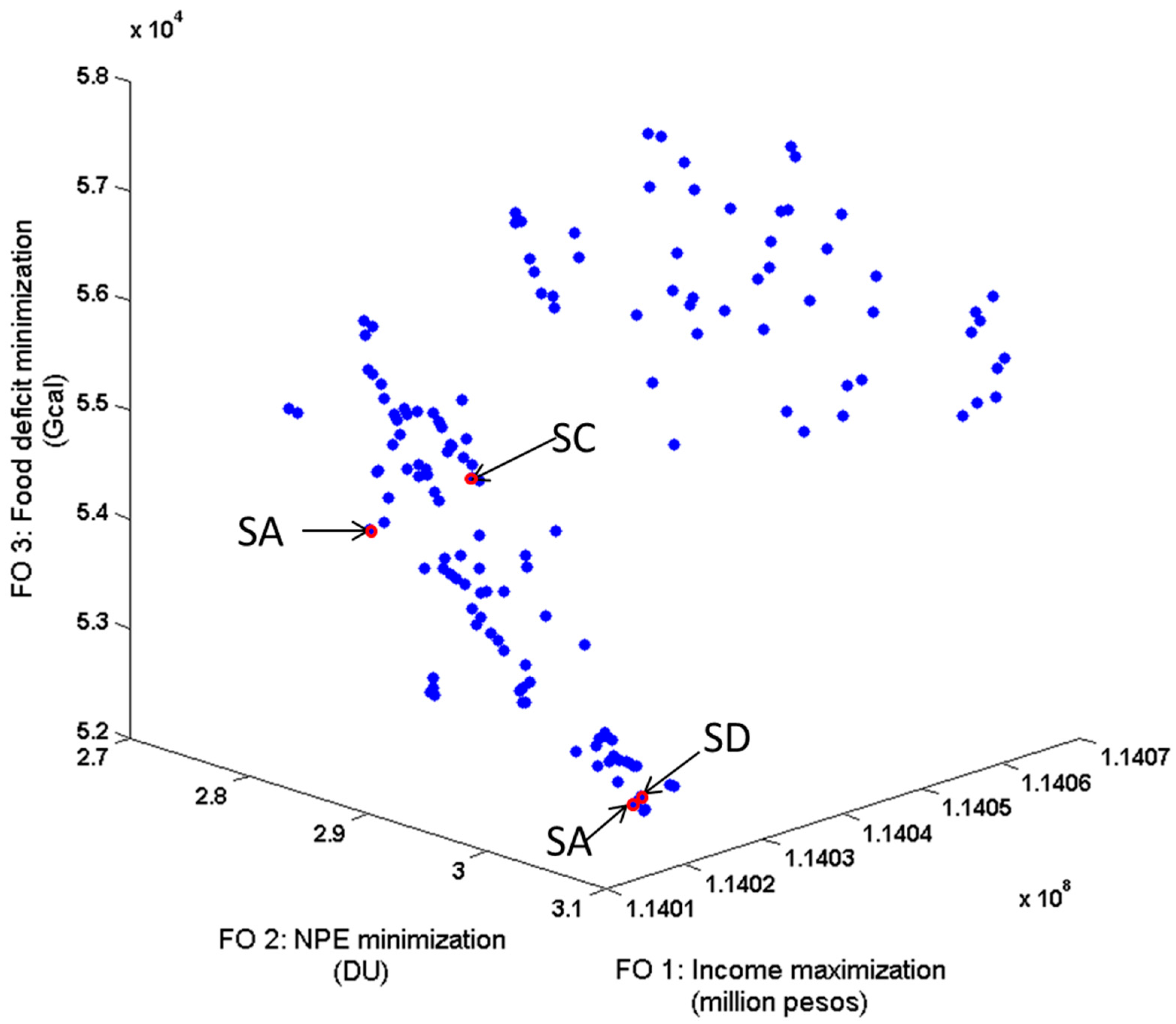
3. Results
3.1. Model Parameters
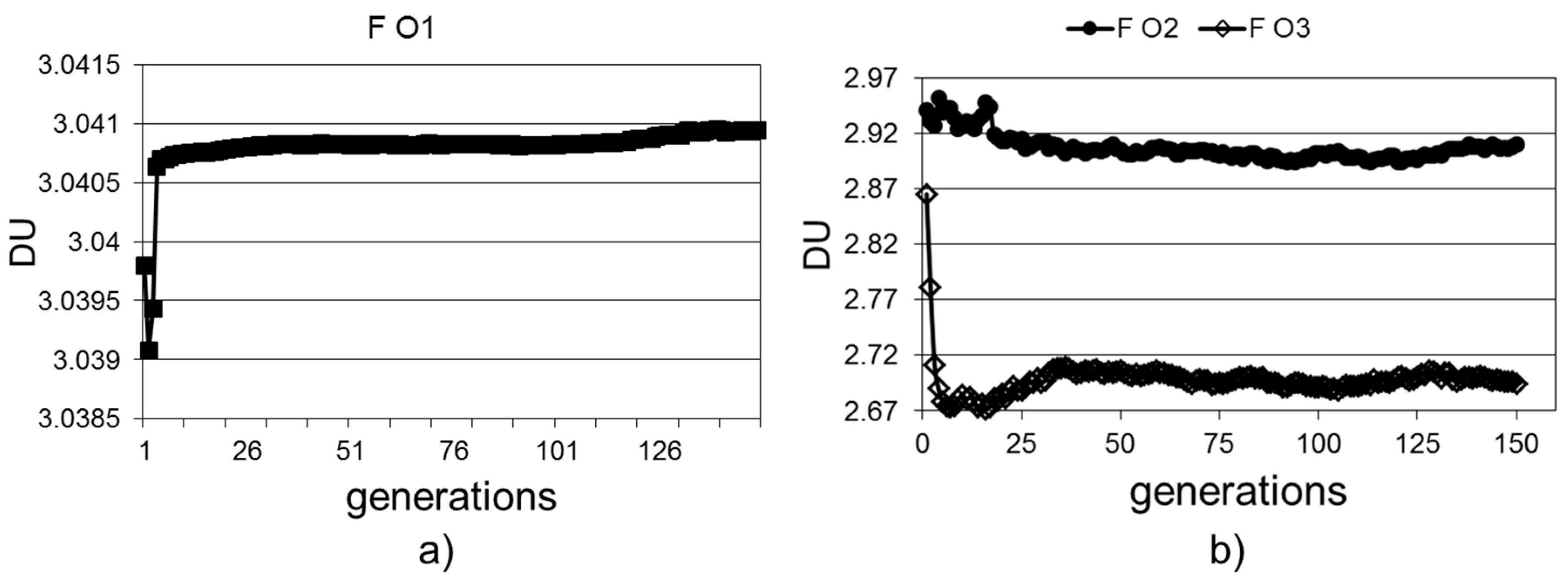
3.2. Evolutive Performance
3.2.1. Global Improvements
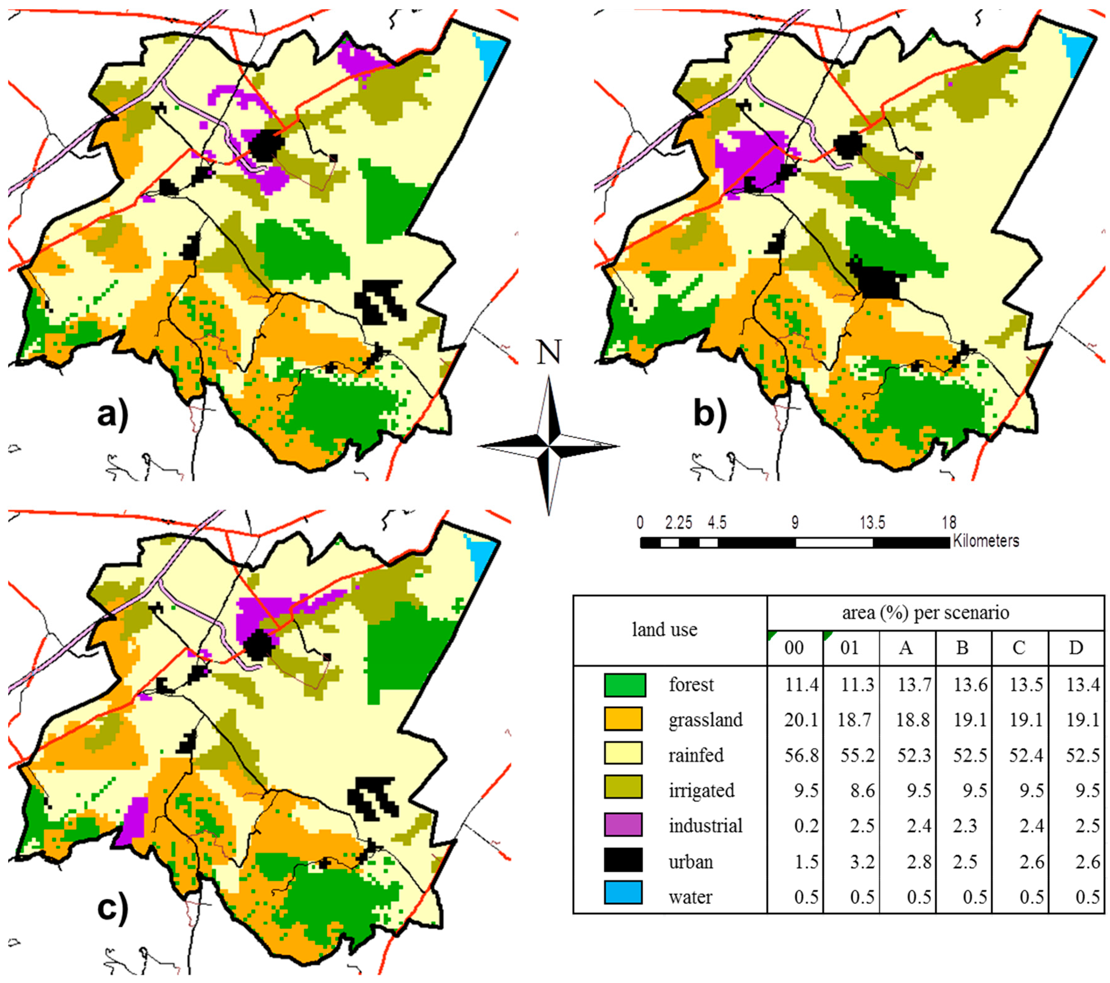
3.2.2. Improvements per Land Use Type
4. Discussion
5. Conclusions
Supplementary Materials
Acknowledgments
Author Contributions
Conflicts of Interest
References
- Laurance, W.F.; Cochrane, M.A.; Bergen, S.; Fearnside, P.M.; Delamônica, P.; Barber, C.; D’Angelo, S.; Fernandes, T. The Future of the Brazilian Amazon. Science 2001, 291, 438–439. [Google Scholar] [CrossRef] [PubMed]
- United Nations Environmentl Programme. Online Version of the Article. The Disappearance of the Aral Sea. Vital Water Graphics, an Overwiew’ of the State of the World’s Fresh and Marine Waters, 2nd ed. 2002. Available online: http://wedocs.unep.org/handle/20.500.11822/20624 (accessed on 9 May 2017).
- Cao, K.; Batty, M.; Huang, B.; Liu, Y.; Yu, L.; Chen, J. Spatial multi-objective land use optimization: Extensions to the non-dominated sorting genetic algorithm-II. Int. J. Geogr. Inf. Sci. 2011, 25, 1–21. [Google Scholar] [CrossRef]
- Stewart, T.; Janssen, R.; Herwijnen, M. A genetic algorithm approach to multiobjective land use planning. Comput. Oper. Res. 2004, 31, 2293–2313. [Google Scholar] [CrossRef]
- Datta, D.; Deb, K.; Fonseca, C.; Lobo, F.; Condado, P. Multi-Objective Evolutionary Algorithm for Land-Use Management Problem. Int. J. Comput. Intell. Res. 2006, 3, 1–24. [Google Scholar]
- Karakostas, S. Multi-objective optimization in spatial planning: Improving the effectiveness of multi-objective evolutionary algorithms (non-dominated sorting genetic algorithm II). Eng. Optim. 2015, 47, 601–621. [Google Scholar] [CrossRef]
- Liu, X.; Ou, J.; Li, X.; Ai, B. Combining system dynamics and hybrid particle swarm optimization for land use allocation. Ecol. Model. 2013, 257, 11–24. [Google Scholar] [CrossRef]
- Jalem, K. Development of water resources for micro watershed at Chinamushidiwada Village in Visakhapatnam, Andhra Pradesh, India. J. Civ. Environ. Eng. 2016. [Google Scholar] [CrossRef]
- Food and Agriculture Organization. Conceptualizing the linkages, Commodity Policy and Projections Service. In Trade Reforms and Food Security; Commodities and Trade Division: Rome, Italy, 2003; Part 1, Chapter 2; pp. 25–34. [Google Scholar]
- Zhang, H.; Zeng, H.; Jin, X.; Shu, B.; Zhou, Y. Simulating multi-objective land use optimization allocation using Multi-agent system—A case study in Changsha, China. Ecol. Model. 2016, 320, 334–347. [Google Scholar] [CrossRef]
- Liu, Y.; Tang, W.; He, J.; Liu, Y.; Ai, T.; Liu, D. A land-use spatial optimization model based on genetic optimization and game theory. Comput. Environ. Urban Syst. 2015, 49, 1–14. [Google Scholar] [CrossRef]
- Schlager, K.J. A land use plan design model. J. Am. Plan. Assoc. 1965, 31, 103–111. [Google Scholar] [CrossRef]
- Chuvieco, E. Integration of linear programming and GIS for land-use modelling. Int. J. Geogr. Inf. Sci. 1993, 7, 71–83. [Google Scholar] [CrossRef]
- Arthur, J.; Nalle, D. Clarification on the use of linear programming and GIS for land-use modelling. Int. J. Geogr. Inf. Sci. 1997, 11, 397–402. [Google Scholar] [CrossRef]
- Malczewski, J. GIS and Multicriteria Decision Analysis; Wiley: New York, NY, USA, 1999. [Google Scholar]
- Balling R, J.; Brown, M.R.; Day, K. Multiobjective urban planning using genetic algorithm. J. Urban Plan. Dev. 1999, 125, 86–99. [Google Scholar] [CrossRef]
- Fernández, I.; Rodríguez, J.A.; Camacho, E.; Montesinos, P. Optimal Operation of Pressurized Irrigation Networks with Several Supply Sources. Water Resour. Manag. 2013, 27, 2855–2869. [Google Scholar] [CrossRef]
- Fernández, I.; Montesinos, P.; Camacho, E.; Rodríguez, J.A. Methodology for detecting critical points in pressurized irrigation networks with multiple water supply points. Water Resour. Manag. 2014, 28, 1095–1109. [Google Scholar]
- Delgado-Osuna, J.A.; Lozano, M.; García-Martínez, C. An alternative artificial bee colony algorithm with destructive–constructive neighbourhood operator for the problem of composing medical crews. Inf. Sci. 2016, 326, 215–226. [Google Scholar] [CrossRef]
- Goldberg, D.E. Genetic Algorithms in Search, Optimization and Machine Learning; Addison Wesley Longman: Boston, MA, USA, 1989. [Google Scholar]
- Ma, X.; Zhao, X. Land use allocation based on a multi-objective artificial immune optimization model: An application in Anlu County, China. Sustainability 2015, 7, 15632–15651. [Google Scholar] [CrossRef]
- Huang, K.; Liu, X.; Li, X.; Liang, J.; He, S. An improved artificial immune system for seeking the Pareto front of land-use allocation problem in large areas. Int. J. Geogr. Inf. Sci. 2012, 27, 922–946. [Google Scholar] [CrossRef]
- Liu, X.P.; Li, X.; Shi, X. A multi-type ant colony optimization (MACO) method for optimal land use allocation in large areas. Int. J. Geogr. Inf. Sci. 2012, 26, 1325–1343. [Google Scholar] [CrossRef]
- Dorigo, M.; Blum, C. Ant colony optimization theory: A survey. Theor. Comput. Sci. 2005, 344, 243–278. [Google Scholar] [CrossRef]
- Mathews, K.B.; Sibald, A.; Craw, S. Implementation of a spatial decision support system for rural land use planning: Integrating geographic system and environmental models with search and optimization algorithms. Comput. Electron. Agric. 1999, 23, 9–26. [Google Scholar] [CrossRef]
- Feng, C.M.; Lin, J.J. Using a genetic algorithm to generate alternative sketch maps for urban planning. Comput. Environ. Urban Syst. 1999, 23, 91–108. [Google Scholar] [CrossRef]
- Buzai, G.D. Análisis Espacial con Sistemas de Información Geográfica: Sus cinco Conceptos Fundamentales. In Geografía y Sistemas de Información Geográfica. Aspectos Conceptuales y Aplicaciones; Buzai, G.D., Ed.; Universidad Nacional de Luján—GESIG: Luján, Argentina, 2010; pp. 163–195. Available online: http://www.gesig-proeg.com.ar/documentos/articulos/2010-BUZAI-CAP7.pdf (accessed on October 24 2016).
- Stewart, T.; Janssen, R. A multiobjective GIS-based land use planning algorithm. Comput. Environ. Urban Syst. 2014, 46, 25–34. [Google Scholar] [CrossRef]
- Porta, J.; Parapar, J.; Doallo, R.; Rivera, F.; Santé, I.; Crecente, R. High performance genetic algorithm for land use planning. Comput. Environ. Urban Syst. 2013, 37, 45–58. [Google Scholar] [CrossRef]
- Cao, K.; Huang, B.; Wang, S.; Lin, H. Sustainable land use optimization Boundary-based Fast Genetic Algorithm. Comput. Environ. Urban Syst. 2012, 36, 257–269. [Google Scholar] [CrossRef]
- Deb, K.; Pratap, A.; Agarwal, S.; Meyarivan, T. A Fast and Elitist Multiobjective Genetic Algorithm: NSGA-II. IEEE Trans. Evolut. Comput. 2002, 6, 182–197. [Google Scholar] [CrossRef]
- Hoekstra, A.Y.; Chapagain, A.K.; Aldaya, M.M.; Mekonnen, M.M. The Water Footprint Assessment Manual. Setting the Global Standard; Earthscan: London, UK, 2011. [Google Scholar]
- Allen, R.G.; Pereira, L.S.; Raes, D.; Smith, M. Crop Evapotranspiration—Guidelines for Computing Crop Water Requirements—FAO Irrigation and Drainage Paper 56 (Spanish Version); FAO: Rome, Italy, 2006. [Google Scholar]
- García, J.; Rodríguez, J.A.; Camacho, E.; Montesinos, P. Linking water footprint with irrigation management in high value crops. Implications on sustainable irrigation agriculture in environmentally sensitive areas. J. Clean. Prod. 2015, 87, 594–602. [Google Scholar] [CrossRef]
- González, R.; Camacho, E.; Montesinos, P.; García, J.; Rodríguez, J.A. Influence of spatio temporal scales in crop water footprinting and water use management: Evidences from sugar beet production in Northern Spain. J. Clean. Prod. 2016, 139, 1485–1495. [Google Scholar] [CrossRef]
- Montesinos, P.; Camacho, E.; Campos, B.; Rodríguez, J.A. Analysis of virtual irrigation water. Application to water resources management in a Mediterranean river basin. Water Resour. Manag. 2011, 25, 1635–1651. [Google Scholar] [CrossRef]
- Dávila, R. Desarrollo Sostenible de Usos de Suelo en Ciudades en Crecimiento, Aplicando Hidrogeología Urbana Como Parámetro de Planificación Territorial: Caso de Estudio Linares N.L. México. Ph.D. Thesis, Fac. Ciencias de la Tierra, University Autónoma de Nuevo León, Nuevo León, Mexico, 2011. [Google Scholar]
- Aller, L.; Bennet, T.; Lehr, J.; Petty, R.; Hackett, G. DRASTIC: A Standarized System for Evaluating Ground Water Pollution Potential Using Hydrological Settings; Research Report EPA/600/2-87/035; Environmental Protection Agency (EPA) Research Laboratory: Ada, OK, USA, 1987. Available online: http://nepis.epa.gov/Exe/ZyPDF.cgi/20007KU4.PDF?Dockey=20007KU4.PDF (accessed on 17 October 2015).
- Menconi, M.; Stella, G.; Grohmann, D. Revisting the food component of ecological footprint indicator for autonomous rural settlement models in Central Italy. Ecol. Indic. 2013, 34, 580–589. [Google Scholar] [CrossRef]
- INEGI. Population Census; INEGI: Mexico City, Mexico, 2010.
- UNAM, INEGI. Inventario Forestal Nacional (National Forestry Inventory) Scale 1:250,000; UNAM, INEGI: Mexico City, Mexico, 2000.
- INEGI. Economic Census; INEGI: Mexico City, Mexico, 2014.
- Méx: SAGARPA; SIAP. Agricultural System Information, (2015) Agricultural Database Years 2004–2014, México. Available online: http://www.gob.mx/siap/acciones-y-programas/produccion-agricola-33119?idiom=es (accessed on 3 March 2015).
- Méx: INEEC, 2013 Inventario Nacional de Emisiones GEI (National Inventory of GHG Emissions). Available online: http://www.inecc.gob.mx/descargas/cclimatico/2015_inv_nal_emis_gei.pdf (accessed on 25 October 2015).
- Méx: SEMARNAT. Programa de Gestión de la Calidad del Aire del Estado de Puebla 2012–2020. 2012. Available online: http://www.semarnat.gob.mx/archivosanteriores/temas/gestionambiental/calidaddelaire/Documents/ProAire%20Puebla2.pdf (accessed on 20 August 2015).
- Audi. Corporate Responsibility Report 2014; Audi AG: Ingolstadt, Germany, 2014; Available online: http://www.audi.com/content/dam/com/EN/corporate-responsibility/audi_cr_report_2014_en.pdf (accessed on 20 May 2016).
- USDA National Nutrient Database for Standard Reference. Available online: https://www.ars.usda.gov/northeast-area/beltsville-md/beltsville-human-nutrition-research-center/nutrient-data-laboratory/docs/usda-national-nutrient-database-for-standard-reference/ (accessed on 10 February 2016).
- WHO: World Health Organization. Estudio Sobre la Necesidad de una Regulación Económica Más Estricta Para Revertir la Epidemia de la Obesidad. BOLETÍN de la Organización Mundial de la Salud. February 2014. Available online: http://www.who.int/bulletin/releases/NFM0214/es/ (accessed on 8 September 2016).
- Nandi, A.K.; Chakraborty, D.; Vaz, W. Design of a comfortable optimal driving strategy for electric vehicles using multi-objective optimization. J. Power Source 2015, 283, 1–18. [Google Scholar] [CrossRef]
- Branke, J.; Deb, K.; Dielrof, H.; Osswald, M. Finding Knees in Multi-Objective Optimization; KanGAL Report Number 2004010; Springer: Berlin/Heidelberg, Germany, 2004. [Google Scholar]


| Land Use | Income per Hectare (Million Pesos) | Annual Income Scenario 00 | Annual Income Scenario 01 | Annual Income | |||
|---|---|---|---|---|---|---|---|
| Scenario A | Scenario B | Scenario C | Scenario D | ||||
| forest | 0.00 | 0.00 | 0.00 | 0.00 | 0.00 | 0.00 | 0.00 |
| grassland | 0.03 | 217.68 | 205.60 | 332.43 | 338.83 | 338.15 | 338.73 |
| rain fed cropland | 0.01 | 147.67 | 143.24 | 128.14 | 127.67 | 124.22 | 127.06 |
| irrigated cropland | 0.02 | 41.03 | 37.23 | 41.19 | 41.19 | 41.19 | 41.19 |
| industrial | 70.82 | 4545.27 | 117,962.90 | 118,516.26 | 117,962.90 | 117,962.90 | 117,962.90 |
| urban | 0.29 | 223.27 | 488.30 | 426.58 | 384.83 | 384.25 | 384.83 |
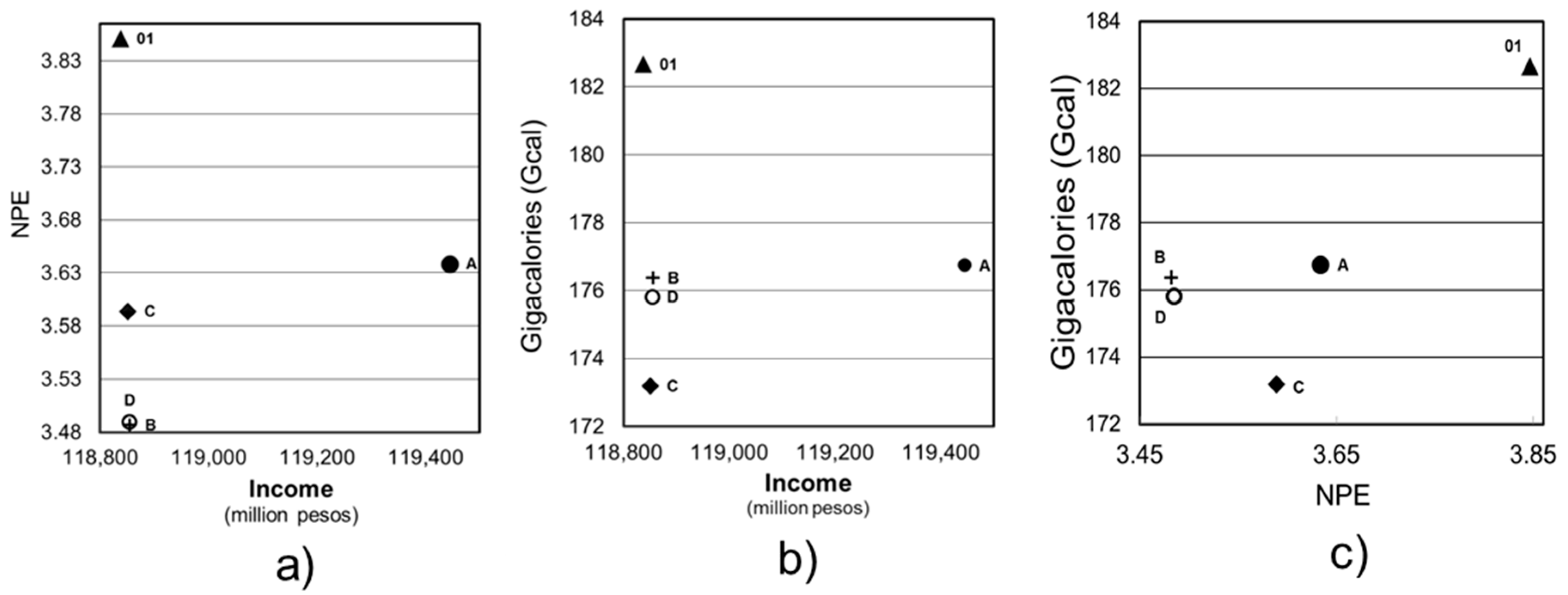
| total | 5174.93 | 118,837.27 | 119,444.60 | 118,855.42 | 118,850.71 | 118,854.71 | |
| Land Use | NPE Scenario 00 | NPE Scenario 01 | NPE | |||
|---|---|---|---|---|---|---|
| Scenario A | Scenario B | Scenario C | Scenario D | |||
| forest | 0.0884 | 0.0884 | 0.0898 | 0.0876 | 0.0877 | 0.0876 |
| grassland | 0.6572 | 0.6075 | 0.5032 | 0.5094 | 0.5102 | 0.5095 |
| rain fed cropland | 1.1049 | 1.0664 | 1.0585 | 1.0724 | 1.0836 | 1.0743 |
| irrigated cropland | 0.0781 | 0.0707 | 0.0781 | 0.0781 | 0.0781 | 0.0781 |
| industrial | 0.7940 | 1.0354 | 0.9985 | 0.9982 | 1.0039 | 0.9985 |
| urban | 0.4282 | 0.9782 | 0.9057 | 0.7364 | 0.8255 | 0.7369 |
| total | 3.151 | 3.847 | 3.634 | 3.482 | 3.589 | 3.485 |
| Land Use | Food Surplus Scenario 00 | Food Surplus Scenario 01 | Food Surplus Optimal Scenarios | |||
|---|---|---|---|---|---|---|
| Scenario A | Scenario B | Scenario C | Scenario D | |||
| grassland | 1.93 | 1.80 | 2.92 | 2.98 | 2.96 | 2.97 |
| rain fed cropland | 120.88 | 115.75 | 103.76 | 103.35 | 100.34 | 102.82 |
| irrigated cropland | 70.83 | 65.12 | 70.06 | 70.04 | 69.89 | 70.02 |
| total | 193.64 | 182.67 | 176.74 | 176.37 | 173.19 | 175.81 |
© 2017 by the authors. Licensee MDPI, Basel, Switzerland. This article is an open access article distributed under the terms and conditions of the Creative Commons Attribution (CC BY) license (http://creativecommons.org/licenses/by/4.0/).
Share and Cite
García, G.A.; Rosas, E.P.; García-Ferrer, A.; Barrios, P.M. Multi-Objective Spatial Optimization: Sustainable Land Use Allocation at Sub-Regional Scale. Sustainability 2017, 9, 927. https://doi.org/10.3390/su9060927
García GA, Rosas EP, García-Ferrer A, Barrios PM. Multi-Objective Spatial Optimization: Sustainable Land Use Allocation at Sub-Regional Scale. Sustainability. 2017; 9(6):927. https://doi.org/10.3390/su9060927
Chicago/Turabian StyleGarcía, Guadalupe Azuara, Efrén Palacios Rosas, Alfonso García-Ferrer, and Pilar Montesinos Barrios. 2017. "Multi-Objective Spatial Optimization: Sustainable Land Use Allocation at Sub-Regional Scale" Sustainability 9, no. 6: 927. https://doi.org/10.3390/su9060927