1. Introduction
Recently, interest in greenhouse gas (GHG) emissions from the dairy sector has been increasing because GHG emissions from this sector are estimated to represent 3%–5% of the global GHG emissions [
1]. All the industry sectors and individual companies in the field of energy, industrial production, agriculture, and wastes in Korea are required to report their GHG emissions to the legal authorities [
2]. Furthermore, Korea began carbon trading in 2015 [
3]. Hence, a more accurate quantification of GHG emissions is required.
Uncertainty analysis estimates the amount of deviation in the calculated output of a mathematical model from its true mean. The results of the uncertainty analysis are often expressed as a confidence interval (CI) at a given confidence level. Quite often, the inputs of the model include observation and/or measurement errors, which reduce confidence in the model output [
4]. In addition to the measurement error leading to parameter uncertainty of the model output, there are other forms of uncertainty, including scenario and model uncertainty. Scenario uncertainty includes choices regarding functional unit, valuation and weighting factors, time horizons, geographical scales, natural contexts, allocation procedures, waste-handling scenarios, use of environmental thresholds and expected technology trends [
5]. Model uncertainty includes models for deriving emissions and characterization factors [
5]. In this study, we focused only on parameter uncertainty.
The Intergovernmental Panel on Climate Change (IPCC) provides good practice guidance on a variety of uncertainty analysis methods [
6]. The methods advocated by the IPCC are listed under Approaches I and II. Approach I refers to the error propagation (EP) method, and Approach II refers to the Monte Carlo simulation (MCS) method.
The EP method used in IPCC’s Approach I does not consider covariance in the variance calculation. However, the MCS method in IPCC’s Approach II considers covariance. Furthermore, Approach II discusses issues of dependence and correlation [
6]. This study considers covariance in all uncertainty analysis methods.
Most of the literature that deals with quantifying GHG emissions in the dairy sector has used the MCS method for uncertainty analysis [
7,
8,
9]. These studies have assumed that all input variables follow parametric distributions, including lognormal and/or normal distributions. Although the MCS method is the method of choice for quantifying uncertainty in the dairy sector, its use for uncertainty analysis has limitations. It requires defining the probability distribution of each input variable, which might be more difficult if empirical information is unavailable [
8]. Basset-Mens et al. [
7] highlighted the difficulties in defining probability distribution for input variables in the life cycle assessment (LCA) studies. Therefore, when the probability distribution of the data points of the input variable is uncertain, other uncertainty methods or probability distributions should be considered, instead of parametric distribution, for analyzing the uncertainty of GHG emissions in the dairy sector.
Because any mathematical model consists of many input variables, an efficient method should be developed to identify the input variables that contribute considerably to the uncertainty of the model output. Global sensitivity analysis or contribution to variance (CTV) approach is an effective tool for this purpose [
10,
11,
12]. The input variables identified as significant to the process become targets for further scrutiny. The results of the sensitivity analysis enable focusing on the identified input variables, such that their observation/measurement errors can be reduced through the use of a larger number of data points. Therefore, the use of the CTV approach simplifies the mathematical model by removing insignificant input variables from the model.
The objective of this study was to compare uncertainty analysis methods for the quantification of uncertainties in the output of the GHG emission model. A linear GHG emission model was formulated to assess the environmental impact of GHG emissions generated at a dairy cow farm in Korea. Two different methods, the MCS and non-parametric block bootstrap (BB), were used to analyze the uncertainty of the GHG emissions model output.
3. Results and Discussion
Data from a dairy cow farm located in Korea were used in the case study to compare the two above-mentioned uncertainty analysis methods [
25]. The number of heads in the dairy cow farm was used to normalize the collected data.
Table 2 shows the normalized initial data, mean, standard deviation (SD), and GHG EF [
26] of the input variables.
A total of 72 monthly data for the input variables were collected. Initially, the most recent 1-year data of the 12-monthly data were used in the uncertainty analysis. Once significant input variables were identified using the 12 data of each of the 11 input variables, the data for 6 years, totaling 72 monthly data of the identified input variables, were used.
The relative errors of the input variables, which is the ratio of the SD divided by the mean, ranged from 31% to 81%, with a simple average of 54%. This indicates that the data variability was not high, being approximately 0.5.
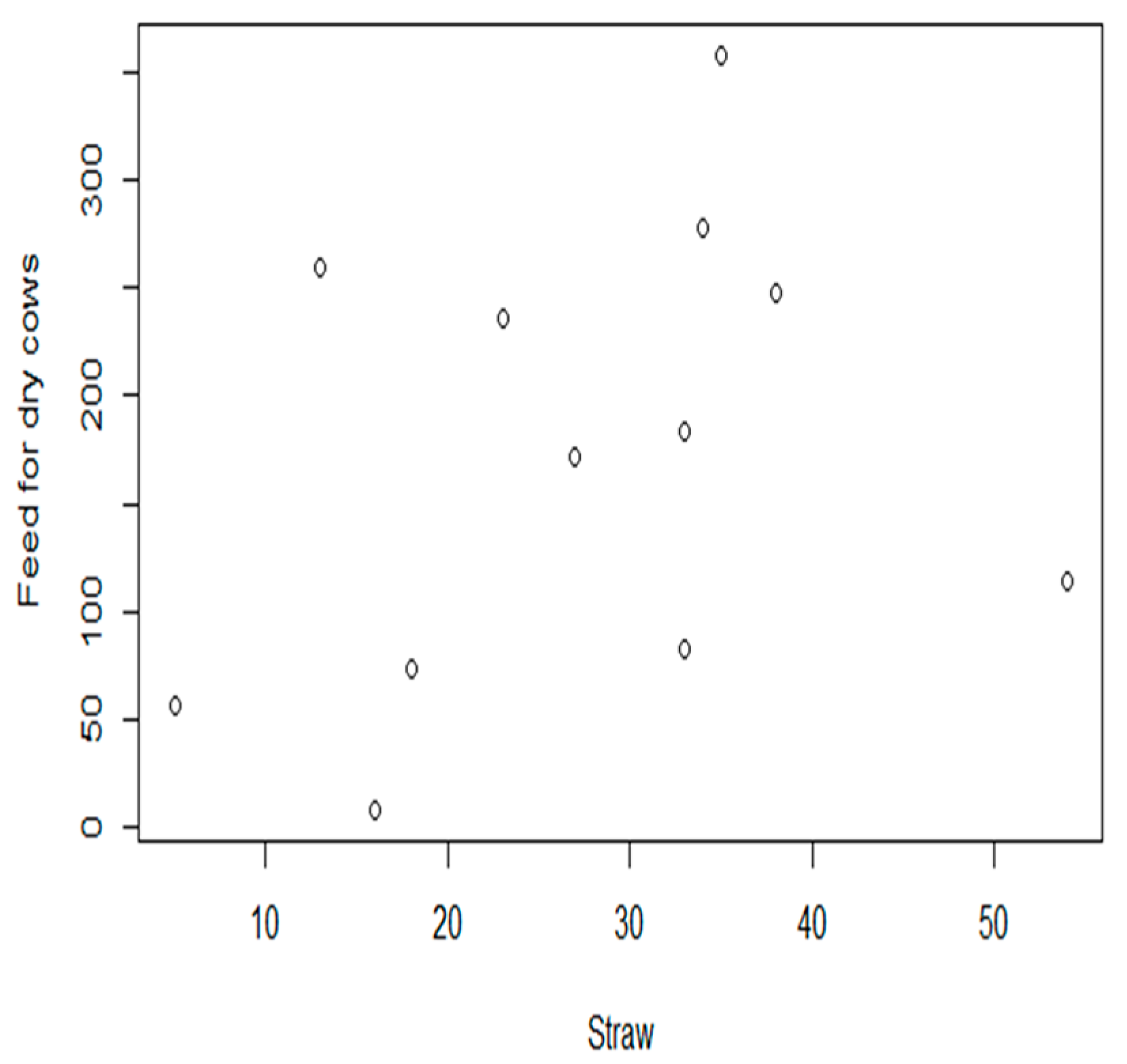
Figure 1 shows the scatter plot of the comparison between feed for dry cows and straw. A correlation was observed between the two variables. Furthermore, a similar trend can be observed among all the input variables. In addition, the covariance between the input variables is not zero, which indicates that there is some degree of association between the input variables. In other words, nonzero covariance implies that the returns of two input variables share some degree of correlation [
27].
The correlation test results for the significant input variables are shown in
Table 3. The results show that there are dependencies among the significant input variables.
The probability distribution of the input variables was evaluated [
28]. The hypotheses for testing the probability distribution using the AD test were as follows. H
0: the input data follow a specified distribution, H
1: the input data do not follow a specified distribution. According to the hypothesis testing of normality, 7 input variables (feed for dry cows, alfalfa, straw, corn silage, rapeseed, bagasse, and electricity) out of 11 showed
p-values greater than the significance level (
, which indicates that they may follow a normal distribution. On the other hand, the probability distribution of the remaining variables showed that three of them (feed for lactating cows, oats, and diesel) may follow a lognormal distribution, with the last one (soybean meal) following a logistic distribution.
Table 4 shows the estimated parametric probability distribution of the input variables with 12 and 72 monthly data points for the MCS method. Dependence among the input variables was taken into consideration by applying the Spearman rank order correlation coefficient in the case of the MCS method. Spearman rank order correlation coefficients were applied to the paired input variables using Oracle Crystal ball software [
29]. Fifty-five correlation coefficients were applied for 11 input variables, whereas 15 correlation coefficients were applied for 6 input variables. Non-parametric probability distributions of the input variables were estimated by using the histogram with data.
In addition, normality plotting (Q–Q plotting) was performed to evaluate the normality of the input variables. However, this plot requires subjective judgment. In the case of seven variables, no conclusive fit could be found to ascertain that they follow a normal distribution. Although the normality test of the input variables using both, the hypothesis test and normality plot, produced positive results, these do not necessarily guarantee normal distribution of the variables. Therefore, there is some uncertainty about the true probability distribution of the input variables.
Covariance is also an important statistic in estimating uncertainty. However, EFs were not treated as random variables in this study. Therefore, only covariance of the input variables was considered in the uncertainty analysis.
Table 5 shows the results of the uncertainty analysis of the GHG emission model for the MCS (with the parametric and non-parametric probability distributions) and BB methods when the number of data points for each input variable is 12.
Table 5 shows that the BB method provides the narrowest CI width and the smallest U value, followed by the non-parametric probability distribution, and parametric probability distribution of the MCS method. The CI width and the U value of the non-parametric probability distribution were approximately 54% and 63% of those of the parametric probability distribution of the MCS method, respectively. Meanwhile, the CI width and the U value of the BB method were 36% and 33% of the CI width of the non-parametric probability distribution of the MCS method, respectively.
Table 6 shows the results of the two uncertainty analysis methods based on the expanded number of data points for the six input variables (
n = 72).
The same trend can be observed in the case of n = 72. This shows that all the statistical values of the expanded number of data points (n = 72) decreased compared to those of the initial number of data points (n = 12). In the case of the BB method, for instance, the percent reduction in the CI width and U value going from n = 12 to n = 72 were 80% and 77%, respectively.
Table 5 and
Table 6 show that the size of CI and the value of U decreases in order, from the parametric MCS to non-parametric MCS method to the BB method. The same trend can be observed with regard to uncertainty of water scarcity footprint (WSF) of a water purifier and rice production in a drainage basin in Korea [
30].
The WSF was calculated using 42 annual data of water resources and water consumption, while the value of U was calculated using the parametric and non-parametric MCS methods, as well as BB method. The value of U with regard to the water purifier using the parametric and non-parametric MCS and BB methods were 118.4%, 103.7%, and 18.9%, respectively [
30]. With regard to rice production, they were 146.0%, 103.0%, and 19.0%, respectively [
30]. There was a significant drop in the value of U and CI from the MCS method to the BB method, although the difference between the parametric and non-parametric MCS was not large.
Decrease in the value of U and CI from the MCS method to the BB method may be due to errors in estimating parametric and non-parametric probability distribution of the input variables for the MCS method. Although non-parametric distribution generates a lower estimate of uncertainty compared to parametric distribution, the difference is minor, which cannot be the basis for claiming that non-parametric probability distribution is preferred over parametric probability distribution in the MCS method. This is mainly because this study is based on a single system with a relatively small number of data points.
Several studies on uncertainty analysis using the MCS method in the LCIA field assumed probability distributions or relied on the judgment of an expert [
7,
8,
31]. Assumed parametric probability distribution or ignoring the covariance of the input variables, would lead to poorer estimation of the variance of the model output, leading to a less accurate estimate of the uncertainty of the model output.
It is premature to conclude that the BB method produces narrower CI and smaller value of U compared to the MCS method in every system. However, this study and the WSF study [
30] showed that the BB method produces a lower estimate of uncertainty compared to the parametric and non-parametric distribution MCS method, most likely due to its distribution-free nature.
The BB method requires many repeated data points of the input variables for resampling. In LCA, we rarely have the ability to measure all input variables repeatedly. Therefore, this is one of the limitations of the BB method. Meanwhile, the parametric MCS method requires probability distribution of the input variable and its parameter values. However, they are often difficult to estimate with accuracy. The non-parametric MCS method requires empirical distribution using methods such as histogram. However, this requires a large number of data points of the input variable. In this study, we have only 12 to 72 data points of the input variable, causing the non-parametric distribution estimated from the use of histogram to be potentially inaccurate.
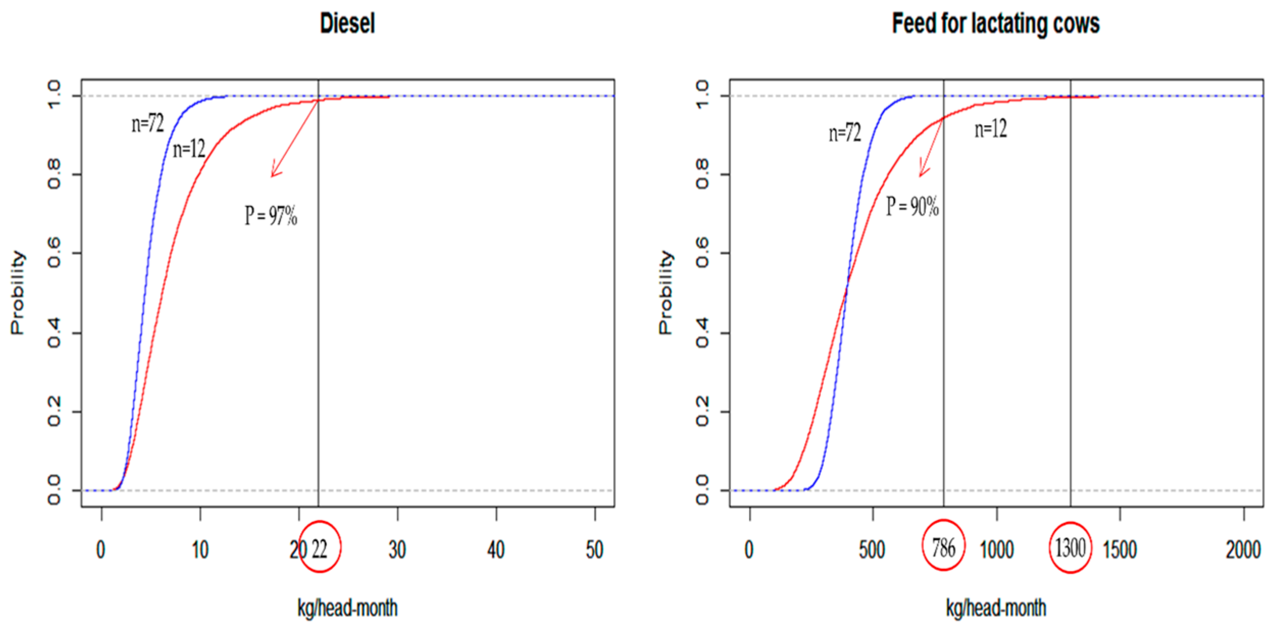
The parametric cumulative distribution (CDF) plot of diesel, shown in
Figure 2, exhibits that there is a 3% probability of exceeding the maximum observed value of 22 kg/head-month when the sample size is small (
n = 12). When the sample size is large (
n = 72), the probability of exceeding the maximum observed value is 0%. The same is true in case of feed for lactating cows.
These results are in agreement with the theory that a parametric fit could better capture the potential for long tails in the probability density functions (pdfs). With regard to the parametric CDF of feed for lactating cows, when n = 12, there is a 10% probability of exceeding the maximum observed value of 786 kg/head-month. However, the parametric CDF predicts a non-zero probability of exceeding 1300 kg/head-month. Normally, a cow farm does not feed the cows this amount. Therefore, this value is considered unrealistic. Thus, parametric probability distribution may produce an erroneous model output, since its pdf includes an unrealistic input value. Meanwhile, non-parametric probability distribution is formulated empirically, based on actual data, preventing the input of an erroneous value.
Table 7 shows the variance of the GHG emission model output, with and without considering the covariance for
n = 12 and 72. The variance was calculated using the EP method.
Since the EP method does not generate a CI, the CI width and U value cannot be computed. This makes the EP method less desirable for uncertainty analysis. The EP method is used to calculate the variance of the model output analytically, which can be used to compare with the variances from the MCS and BB methods.
The variance of the GHG model calculated using the EP method shown in
Table 7 was 34,013, by considering covariance (it was 19,726 without considering covariance) when
n = 12. The variance of the model output from the BB and non-parametric probability distribution of the MCS methods, when
n = 12, were 31,053 and 25,730, respectively. These three variance values are similar to each other. Meanwhile, the variance with the parametric probability distribution of the MCS method when
n = 12 was 100,827, which is approximately three times greater than those of the other three results. The same trend can be observed when
n = 72. Thus, the parametric probability distribution method appears to overestimate the variance of the GHG model output.
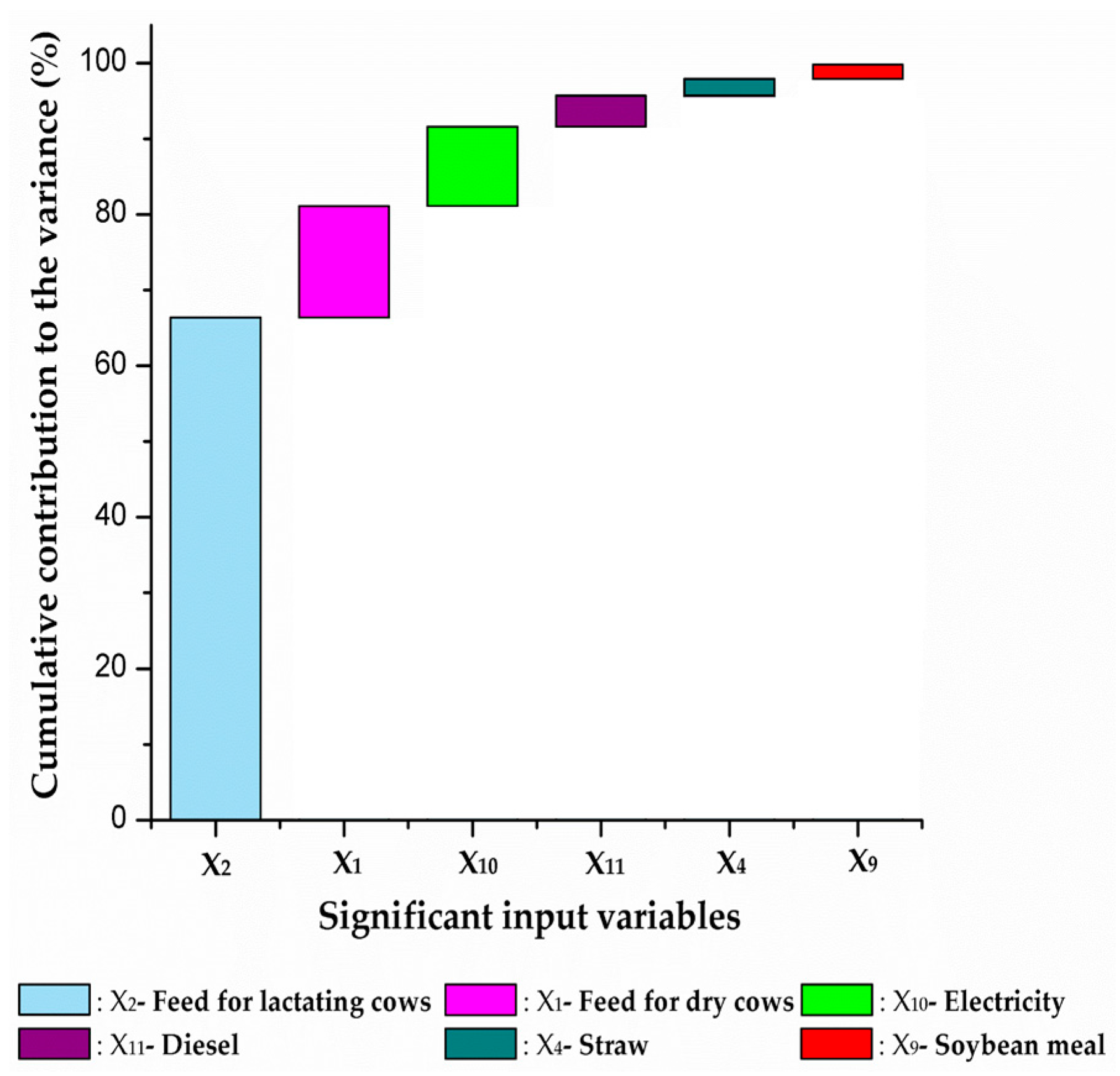
The EP method can be used for the CTV analysis to identify the input variables that contribute considerably to the total variance of the model output.
Figure 3 shows the cumulative contribution of the 6 input variables based on the initial data of 11 input variables, namely 99.8% of the total variance. The variance of the feed for lactating cows contributed the most, followed by the feed for dry cows, electricity, diesel, straw, and soybean meal. Therefore, these six variables were selected as the targets for the expanded data collection, with
n = 72. On the other hand, the contributions of the remaining five variables to the variance of the model output were considered negligible.
It is well-known that a higher number of data points reduces the variance of the mean, also lowering the uncertainty of the model output. The finding in this study is that the CTV approach can minimize the number of input variables for collecting an expanded number of data points. For example, in this study, if the input variables would be limited to those contributing at least 95% to the model output variance, the number of input variables for the expanded data collection would be reduced to four (feed for lactating cows, feed for dry cows, electricity, and diesel).
Both, the activity data and the EFs, influence the uncertainty of the model output in LCIA [
7,
8,
31]. However, this study did not treat the EFs as random variables, which is its limitation. The reason for treating EFs as a constant was that the EFs derived from the Korean LCA database have many shortcomings from a statistical standpoint (e.g., fewer studies, limited number of data points, less transparent system boundaries of the LCA studies, etc.).
When EF is treated as a random variable in addition to the current input variable in this study, the GHG emission model contains two independent random variables. In this case, the bootstrapping method can be applied by resampling both variables separately, subsequently taking the average of the resampled data of each variable and multiplying the two averages to generate the GHG emission value. By repeating this procedure, say, 1000 times, the average GHG emission values are used to produce 95% CI of the GHG emissions using the percentile method.

 ,
, 

