1. Introduction
Evapotranspiration plays a key role in the Earth’s surface energy and water balances, and it has substantial effects on global climate change, water management and crop yield [
1,
2,
3]. Satellite-based remote sensing has been identified as a suitable means of mapping the spatial distribution of ET or LE. Because of technical and methodological limitations, many remote sensing-based ET or LE models have been conducted under quite homogeneous and flat conditions, with the use of decametric to kilometric spatial resolution sensors [
4,
5]. However, the Earth’s surface geometry, physical processes and associated variables are inherently heterogeneous. Due to the nonlinear nature of many land surface processes, heterogeneity can profoundly affect the result of estimating ET or LE [
1,
6].
The effect of surface heterogeneity on remote sensing-based ET or LE estimation is mainly caused by two aspects: the heterogeneity produced by the landscape and the heterogeneity produced by surface variables [
1]. Three basic types of methods have been proposed to compensate for the errors caused by surface heterogeneity or considering subpixel scale land surface heterogeneities when estimating surface ET or LE [
7,
8,
9,
10,
11,
12]. The error caused by the landscape heterogeneity is usually corrected using the mosaic or area weighting method [
1,
11] and the correction factor compensation method [
13]. The mosaic or area weighting method neglects all small-scale interactions by dividing each grid cell into several homogeneous patches according to the different land-use types, assuming that the various patches do not interact with each other but interact vertically with the atmosphere directly above them [
14]. The grid fluxes are the averages of the patch fluxes weighted by their fractional area no matter where within the grid cell the individual patches are located [
9,
15]. Therefore, in the same landscape, the errors caused by the heterogeneity of spatial patterns change of the surface variable are negligible for the ET or LE calculation. The error caused by the heterogeneity of the surface variables (i.e., land surface temperature (LST)) is usually corrected by the temperature-sharpening method [
1,
16], and it is capable of decreasing the influences of the heterogeneity of the LST [
17,
18]. The core of these two methods is to combine the high-resolution satellite data with the low-resolution satellite data and using statistical methods to describe and express the heterogeneity of the landscape composition or the spatial distribution of the variables in the mixed pixel to correct the ET or LE estimation error. In addition, the physical mechanisms of some methods (e.g., the correction factor compensation method) are not clear, leading to low portability [
13,
19].
Therefore, the study of surface heterogeneity in ET or LE estimation from the perspective of remote sensing model is still needed. The method of using frequency distributions or generalized probability density functions (PDF), which is called the “statistical-dynamical” approach, to describe the variability of land surface characteristics is a good way to solve the problem [
10,
20,
21,
22]. It is based on the assumption that climate forcing (temperature, precipitation, humidity, etc.) and land surface characteristics (i.e., soil, vegetation, topography, etc.) vary according to the distributions which can be approximated by continuous analytical PDFs rather than a single representative value. The grid fluxes are calculated by statistical-dynamical method using numerical or analytical integration over appropriate PDFs [
23]. Li and Avissar [
10] demonstrated that the results of determined fluxes depend on the spatial distribution of the land surface parameters, and the more skewed the distribution within the range of values, the larger the error (for nonlinear relationships) of the flux calculated using the mean instead of the distribution. Tittebrand and Berger [
14] confirmed the possible application of the PDF-approach for the determination of LE with Penman-Monteith using Normalized Difference Vegetation Index (NDVI), albedo, relative humidity and wind speed for grassland and coniferous forest. The PDF-based flux estimation model can be used to describe spatial variability of specific surface parameters for a model grid or a satellite pixel with coarser spatial resolution that is described by a higher resolved dataset [
10,
14,
20,
21,
22,
23].
The appropriate choice of spatial heterogeneity description method based on different usages is the key to eliminate ET or LE estimation error. The heterogeneity produced by landscape is often expressed by a landscape pattern index including Moran’s I spatial autocorrelation index [
24], Getis statistics [
25], porosity indices, etc. The heterogeneities of surface variables are regarded as two different aspects with or without considering the spatial patterns of surface variables [
26,
27]. By considering spatial patterns or spatial arrangement as well as the value of the gray scale of the pixels, the changes in spatial patterns with more or less chaotic spatial arrangements correspond to greater or smaller spatial heterogeneity [
2,
10]. In the other way, only the heterogeneity caused by the change in the variable value or gray value (i.e., spatial variability of the surface property over the observed scene) is considered [
26]. Correspondingly, the description of spatial heterogeneity contains two groups of methods. One group considers both the spatial patterns and spatial variability of the variable, including empirical, probabilistic and other methods. Empirical approaches such as local variance [
28], Haralick indices [
29] and ANOVA-quadtree analysis [
30] may be limited in charactering the image spatial heterogeneity because of the lack of an underlying theoretical framework [
26]. Probabilistic approaches (e.g., spatial entropy, multifractal, fractal, variogram [
31], and q-statistic method [
27]), which consider the image as a realization of the stochastic process called random function [
26], provide more efficient tools to model the spatial heterogeneity of components. Other methods involve mathematical models such as wavelet analysis [
19] and Fourier transform [
32]; moreover, geographically weighted regression has become popular to explore spatial heterogeneity [
33]. These methods are mostly used to analyze the heterogeneity of land surface solely, so the spatial patterns of pixels and spatial variability of the variable values both need to be considered [
26,
34]. The other group focuses only on spatial variability of the variable values and does not consider the spatial patterns. The commonly used methods include the quantile, range, deviation, variance/standard deviation, moment, coefficient of variation (CV) [
25], Gini coefficient and entropy [
34,
35], and these methods are often used for specific purposes (e.g., building models) [
36].
Though most PDFs are described by only a few parameters, implementing a PDF for each land-surface characteristic would greatly increase the complexity of this type of parameterization, as well as the computational burden of the model [
10]. Therefore, in attempting to produce efficient PDF-based parameterization of remotely sensed ET or LE, one needs to solve a basic question: which surface variables’ heterogeneity must be considered when establishing an ET or LE estimation model, i.e., which variability of surface variables varies similarly or consistently with the variability of the turbulent flux in time. Since the use of PDF alone does not facilitate direct comparisons of the spatial variability of surface variables, in order to answer the question, an index that quantitatively describes the overall variability of the PDF is still required [
37]. The main objective of this study is to find an index to describe the heterogeneity caused by the fluctuation of the surface variable values, i.e., the spatial variability of the surface variables over the observed scene. Based on simulation data and Heihe Watershed Allied Telemetry Experimental Research (HiWATER) data, we used the PDF as a starting point to explore the spatial variability expression method of surface variables, and this approach could be used to systematically analyze the spatial variability of surface variables and compare the variability of different variables over the same observed scene.
3. Methodology
The remote sensor above the land surface receives not only the signal of the mean and variance but also the signal of all values present on the surface. Thus, modelers are especially interested in the PDF of the surface variable [
14,
34], which tells how frequent a certain parameter value occurs. For the same variable, if the PDF is narrow, then the surface is more homogeneous, and if the PDF is broad, the surface is more heterogeneous [
34]. PDF can describe heterogeneity in a qualitative manner, however, it is unable to quantify the information content and cannot be used to compare the variability of different variables over the same observed scene [
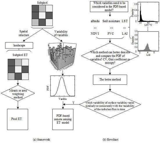
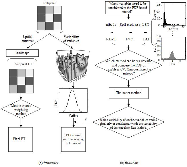
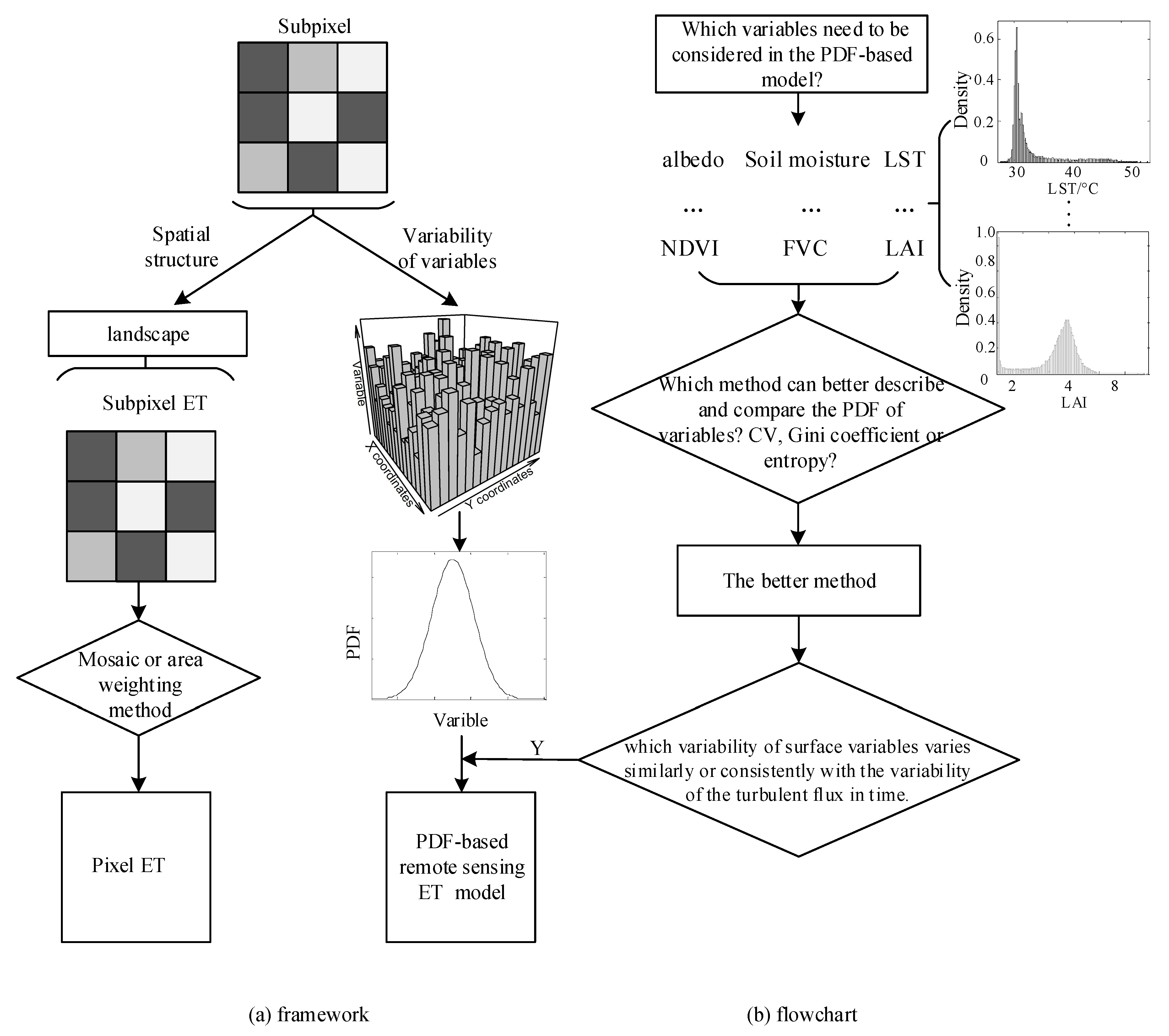
34]. As we mentioned in the introduction, the commonly used methods that express the spatial variability of surface variables include the quantile, range, deviation, variance/standard deviation, moment, CV, Gini coefficient and entropy. Because the magnitude and dimension of each surface variable vary, a dimensionless or dimensional consistent indicator is required to compare the variability between variables directly. After comparing the aforementioned methods, the indicators that can satisfy the above demand and better represent the variability are the CV, Gini coefficient and entropy. The first two are dimensionless. For a fixed scale, the amount of information can be quantified via the entropy and its dimension is consistent; the unit in this paper is nats. We illustrate the characteristics of the three methods in expressing spatial variability from both aspects of simulated data and experimental data. The framework and flowchart of this paper is shown in
Figure 2. PDF is the starting point for our research of surface spatial variability. The framework in
Figure 2 is as we reviewed in the introduction, and for the flowchart (i.e., the main purpose of this paper), it is the first step to answer the basic question, and also the first step to build a more efficient PDF-based ET or LE estimation model. The details of the three methods are described in the following paragraphs.
CV is dimensionless and often used for auxiliary modeling, such as the use of CV to characterize surface variability when establishing a temperature-sharpening method, and lower CV values correspond to more homogeneous land surface values [
1,
3,
36]. CV can evaluate the variability of a sample in a population as follows [
25]:
where std(x) and u(x) are the standard deviation and the average value of the sampling point, respectively. u(x) can be negative, then the above equation is also negative. However, if CV is negative, its absolute value should be used to measure the degree of variability (i.e., the greater the absolute value, the stronger the degree of variability, and vice versa). Generally, a value of CV < 0.15 indicates a variable with low variability; 0.15 ≤ CV ≤ 1 indicates a variable with moderate variability; and CV > 1 indicates a variable with a high degree of variability [
1,
36].
Compared to CV, the Gini coefficient is also dimensionless and is more likely to represent the ratio of deviations between data [
44]. The Gini coefficient is an index of the fairness of the income distribution in the field of economics, and it is in the range of [0, 1]. For n values of the variable x, a number of methods are available to calculate the Gini coefficient. The calculation method used in this study is as follows [
44]:
Information entropy is a state variable in thermodynamics that indicates the degree of chaos, and it was introduced into information theory by Shannon (sometimes called Shannon entropy) and now represents a measure of the uncertainty of a random variable. The random variable is divided into several intervals, each of which represents a state of the variable, and entropy is the average uncertainty of all possible states of the variable. It is also a common tool to quantify the information included in the PDF [
34,
45]. For discrete data, the formula is as follows [
46]:
where p
i is the probabilistic mass function (PMS) of the variable that falls within the
ith interval after dividing the set of points into n intervals, and it satisfies the normalization condition
. The calculation of entropy is related to the size and the start of the probability density interval segmentation, and Brunsell, Ham and Owensby [
35] suggested using the kernel density estimation method to determine the interval size and the starting value. In this paper, we used the Gaussian kernel density estimation method to divide the interval into 512 aliquots and calculate the probability [
47]. When the variable has only one state or a single value distribution, the entropy value is 0; and when the variable is evenly distributed, the entropy value of the variable is the largest, which is ln
n.
Because the number of observations involved in the calculation of each variable varies, in order to make the variability of each variable comparable, the entropy of all variables must be normalized, and the formula is as follows:
where m is the number of observations.
The above three methods are often used in remote sensing-assisted modeling [
1,
3,
34,
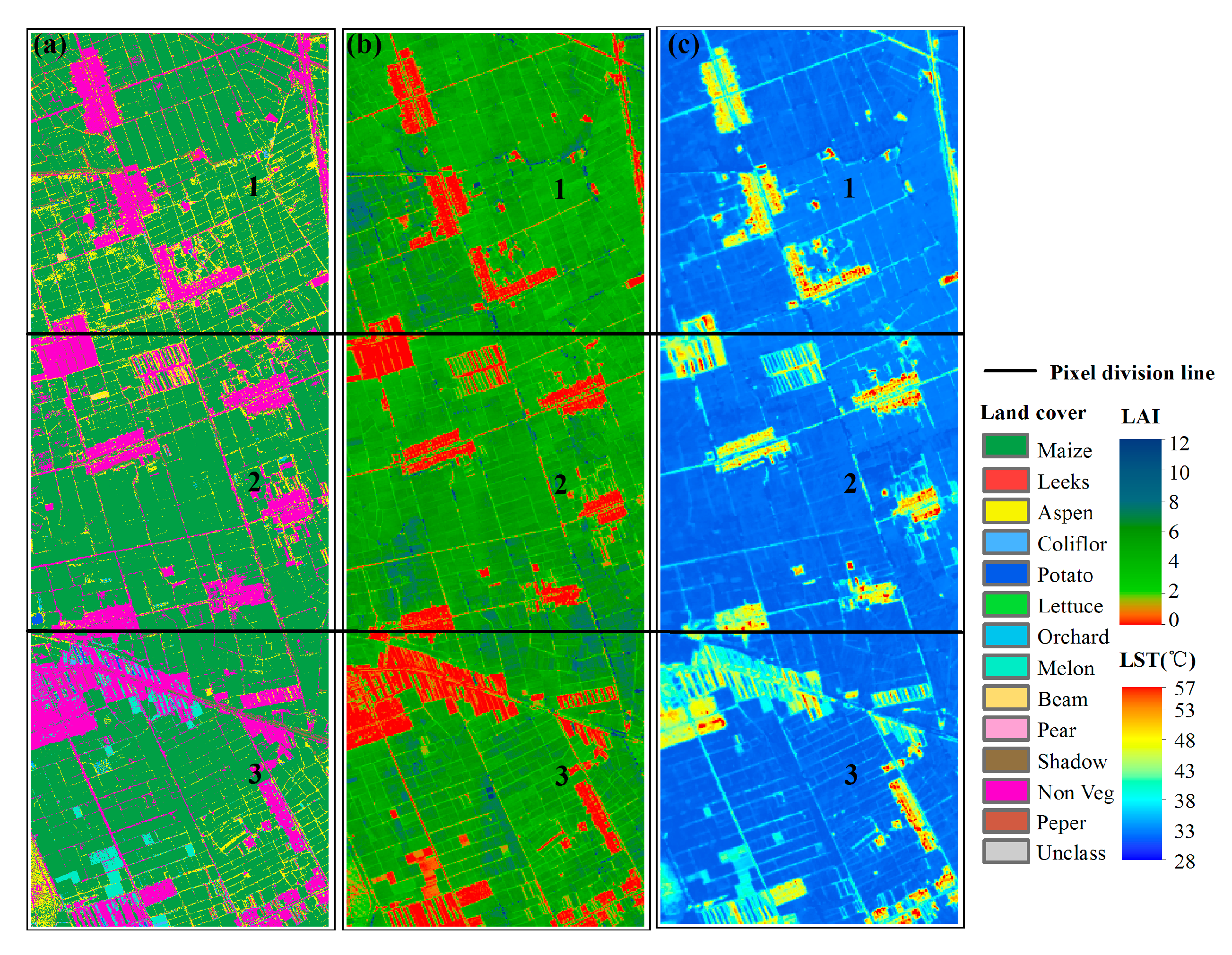
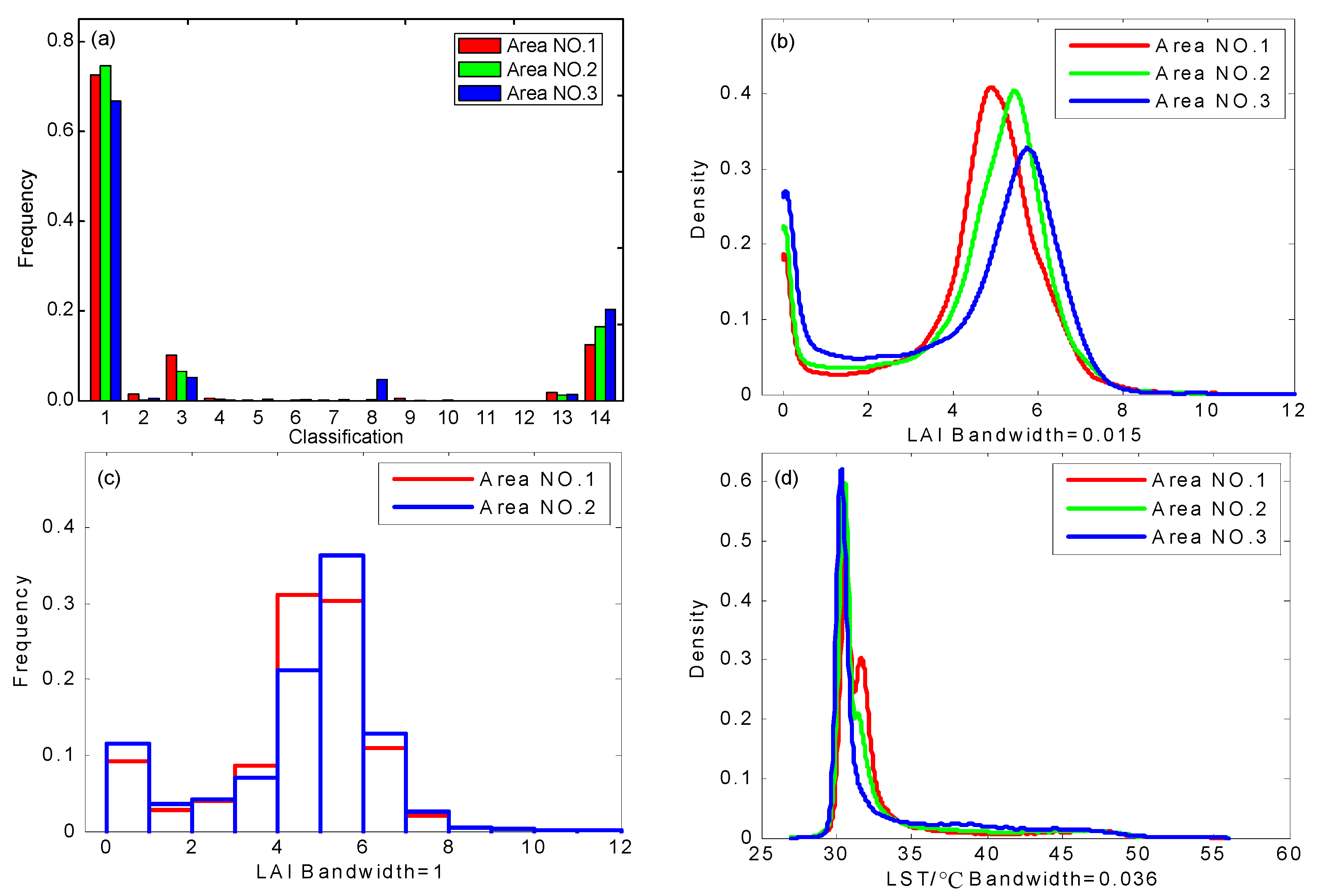
44]. Therefore, compared with other methods (i.e., quantile, range, deviation, variance/standard deviation and moment) the three methods are not only dimensionless or dimensional consistent, but also have representativeness. In this paper, we analyze the three methods from different type of data (e.g., remote sensing airborne data) to express variability.
5. Discussion
The entropy describes the spatial variability much better than CV and Gini coefficient. Generally, the CV and Gini coefficient have similar characteristics when expressing spatial variability, but the Gini coefficient is more focused on the deviation ratio between data. Therefore, in some cases, the Gini coefficient is worse than the CV in expressing spatial variability, and the Gini coefficient has a large computational effort. In summary, the advantages of entropy are described as follows:
Entropy is more consistent with PDF when describing spatial variability, and in some extreme distributions, entropy can express spatial variability more accurately, while CV and Gini coefficients cannot.
In this paper, the unit of entropy is nats, which can be used directly to compare the spatial variability of variables. While the CV and Gini coefficients cannot, they are affected by the specific value (i.e., the average) of the variable.
Nevertheless, it is worth mentioning that PDF is the starting point for our research of surface spatial variability. If we do not use this as a prerequisite to analyze the heterogeneity of surface variables separately, the spatial patterns (also known as spatial structure) or spatial autocorrelation of the surface must be considered [
26,
34]. Entropy calculates the variability of variables in their own range. In
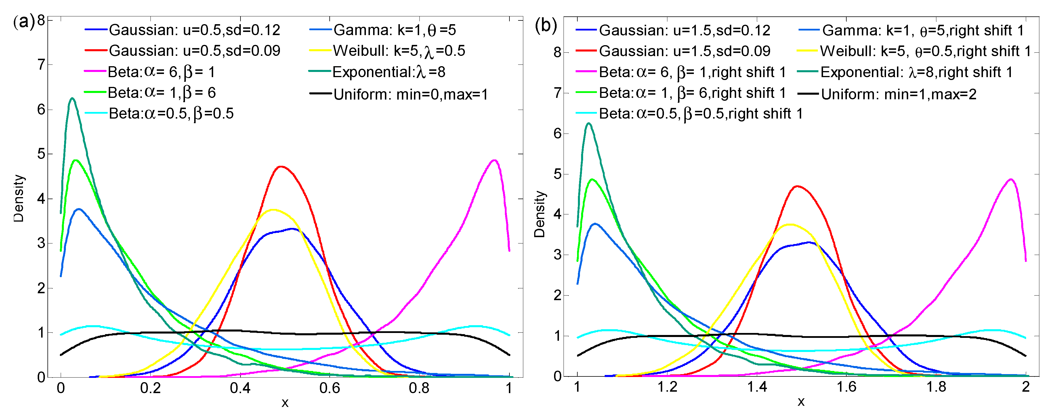
Table 1, if we compare the three methods in describing the variability between the different distributions, the result is still reliable. However, we must consider the actual range of variables. For example, if variable A satisfies a uniform distribution, its value can range from 0 to 10, and in some cases (e.g., an observation scene of a remote sensing image or the target area that we are interested in) its value falls in the range of 0–1. If there is no value in the 1–10 range, similar to U (1) in
Table 1, then its variability is not necessarily stronger than variable B which belongs to other distributions (e.g., the beta distribution in
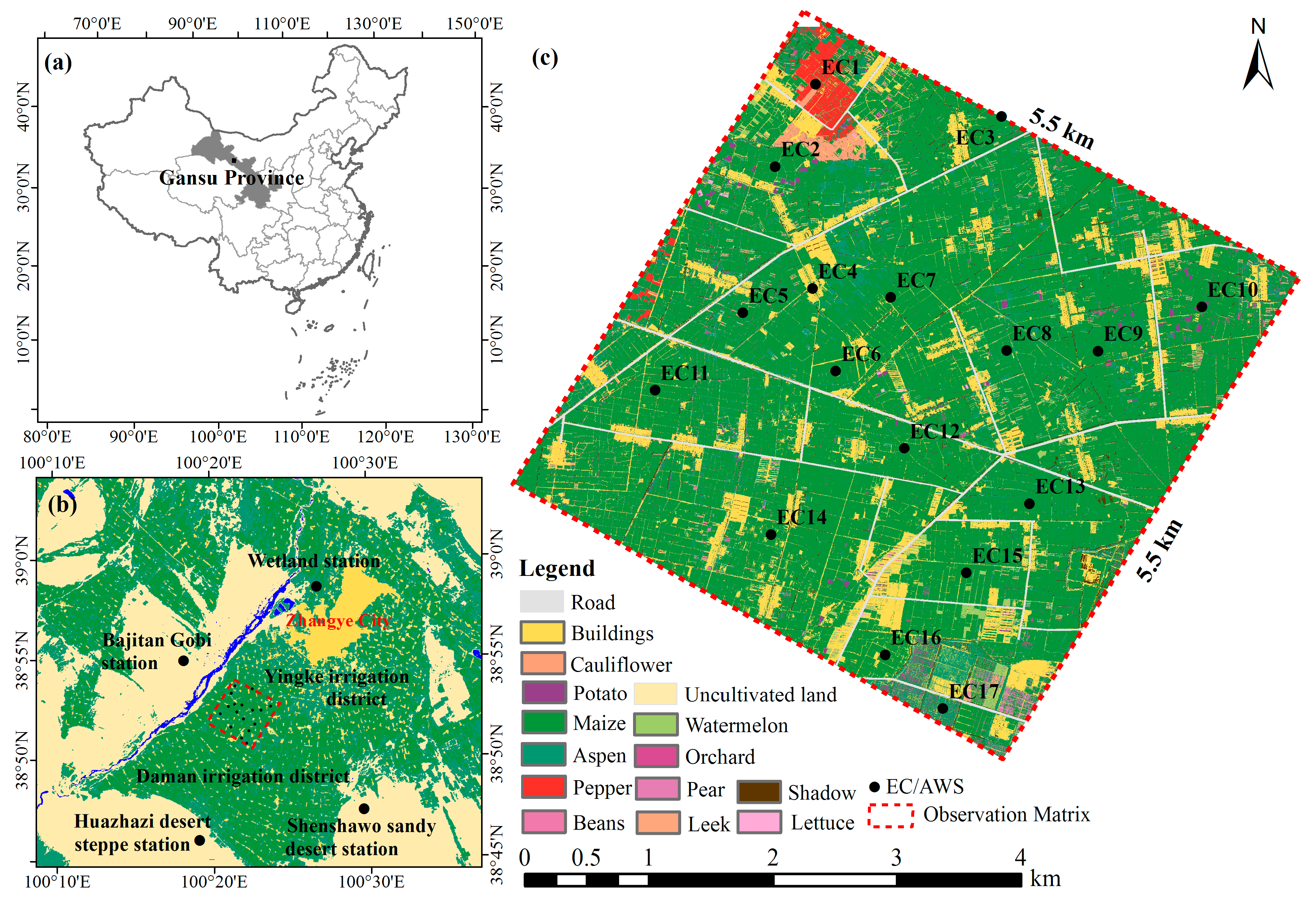
Table 1) in the actual sense. In this article, the design and arrangement of the scheme is to gradually illustrate the characteristics of the three methods in expressing spatial variability. In addition, entropy takes into account the distribution of variable values, and its calculation has a certain dependence on the number of samples. Considering the high cost of the experiments, the datasets of the seventeen EC systems and AWS stations in the 5.5 × 5.5 km
2 kernel experimental area are very valuable [
39]. Moreover, the conclusions drawn from the analysis based on the spatial data may be quite preliminary but are important and valuable for future exploration in this area. More data from wireless sensor network [
49] will be added and used for more sophisticated analysis. More reliable and interesting findings will be discovered with increased number of sites and observations. Detailed information on the spatial variability of variables derived from the ground observation network and the time variation of the variability of surface variables will be introduced in another paper.
6. Conclusions
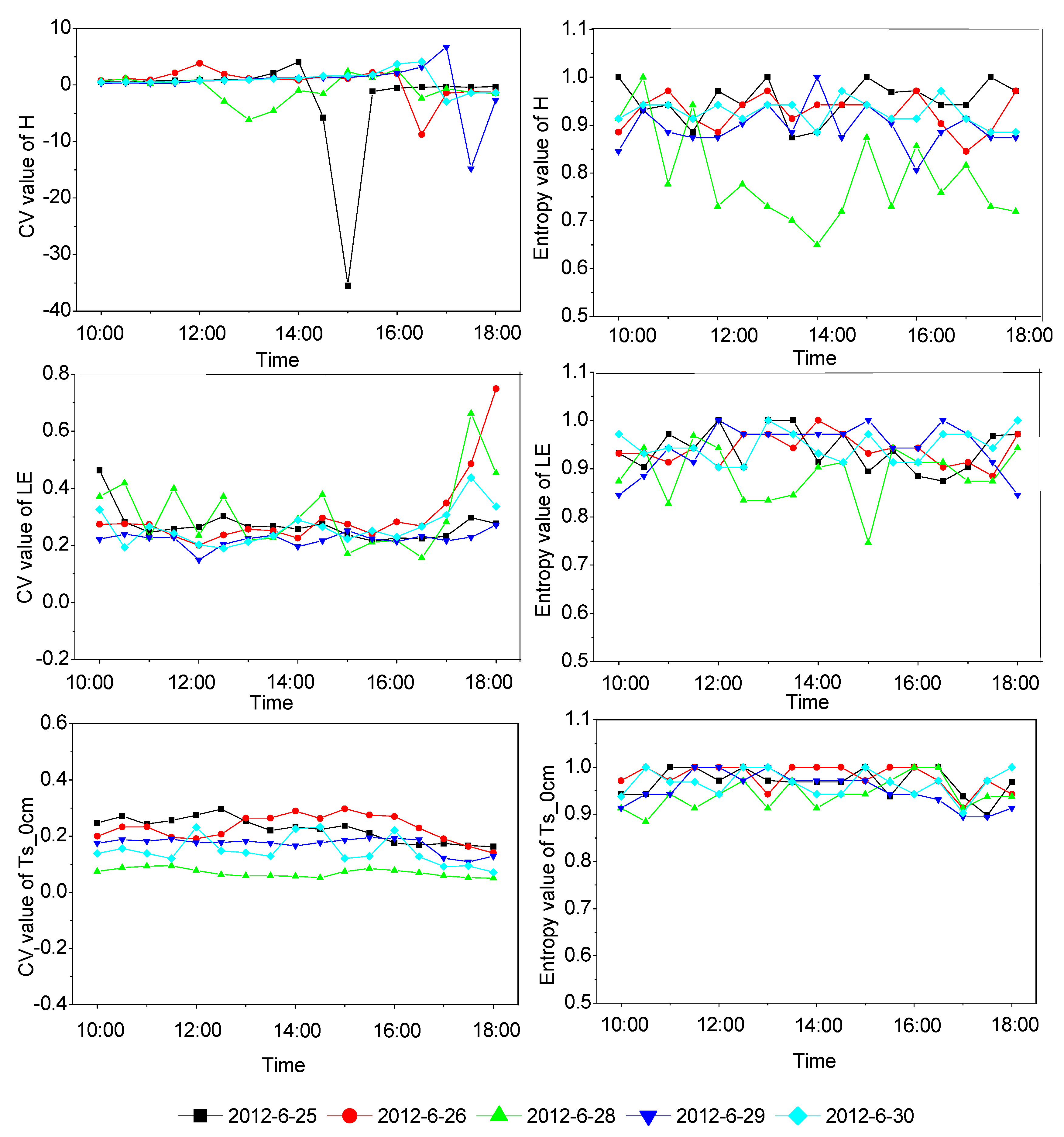
The estimation of ET or LE using remote sensing data does not usually consider the influence of advection or interaction between subpixels; hence, the distribution of surface variable values (i.e., spatial variability) is usually the focus for building a model that considers the heterogeneity produced by surface variables for a target area or landscape. PDF is the most promising way to describe subpixel variability for given data. In attempting to produce efficient PDF-based parameterization of remotely sensed ET or LE, it is important to determine which variables are similar or consistent with the variability of turbulent flux in time. However, the use of PDF alone does not facilitate direct comparisons of the spatial variability of surface variables. To address this, we chose three dimensionless or dimensional consistent indicators, i.e., CV, Gini coefficient and entropy values, to express the variability in surface variables. Based on the analysis of simulated data and the field experiment data, we found the following: (1) Entropy has a high consistency with the PDF of surface variables, which is more stable and efficient in expressing the variability of surface variables. The entropy of the airborne data shows that the variability of LAI is greater than that of LST; (2) Regardless of whether it is from the analysis of simulated data or field experimental data, the CV and the Gini coefficient are insufficient for measuring spatial variability. They are susceptible to the mixing of special values, such as the inversion of temperature at the oasis in the summer; (3) The results of normalized entropy of different variables observed by EC systems and AWS stations show that the variability of soil moisture at depth of 2 cm (MS_2cm) is the strongest, and the variability of friction wind speed (Ustar) is relatively strong, which is related to the special geographical environment of the study area. Furthermore, the trend of sensible heat flux (H) and latent heat flux (LE) seems to show a certain diurnal variation.
The findings of this study provide a reference for expressing the spatial variability of surface variables and illustrate a suitable method for comparing the variability of different variables. How to combine it with the analysis in which surface variables vary similarly or consistently with the variability of the turbulent flux in time and to establish a more efficient PDF-based remote sensing ET or LE model will be the next research goal.

 ,
, 


