3D Vibration Estimation from Ground-Based Radar

Abstract

The paper proposes a method to estimate 2D/3D vibrations and displacements of mostly linear structures, like pipes, chimneys, towers, bridges from afar, based on synchronized Radars. The method takes advantage of Radar sensitivity to displacements to sense tiny deformations (up to tens of micron) with a time scale from milliseconds to hours. The key elements are: (a) The use of calibrators to remove at once both the tropospheric turbulence and the effect of radial motion, and (b) the compensation of interferences from fixed targets. The latter is performed by estimating and removing the contribution of interfering targets, based either on a proper data processing or by exploiting an ad-hoc motorized calibrator. Performance in terms of accuracy of the deformation field is evaluated theoretically and checked by tests carried out in laboratories and by full-scale acquisition campaigns.

1. Introduction

The use of Radar for remote monitoring of vibrations and displacements in structures, infrastructures, and buildings has become more and more widespread thanks to the advent of small, cost-effective devices, combined with their intrinsic advantages due to a fast installation that avoids wiring, a sensitivity to vibrations from frequency zero to kHz, and a wide dynamic range [1,2,3,4,5,6,7,8,9,10,11].

Most Radar-based systems are designed for bidimensional imaging, like rail-mounted Synthetic Aperture Radar (SAR) or Multiple Input Multiple Output (MIMO) Radar [12,13]; however, simple monodimensional (1D) Radars are used in many applications—particularly for Short Range Radar (SRR), thanks to the fine range resolution that allows us to separate echoes coming from objects extended in a predominant direction, like in pipes, chimneys, towers [1,2,3,6,7,8,10,11], and, most noticeably, cable-strayed bridges [10,14,15].

In these cases, we propose a combination of just three such Radars, properly synchronized to avoid interfering with each other, allowing for a complete 3D rendering of the displacement of each target. The drawback of such a simple system is the interference coming from stable or moving targets placed in the same range, but different azimuth or elevation, like from the ground or other structures.

In this paper, we discuss a system made up of up to three Radars for precise remote estimation of vibrations and displacements in 3D; in particular, we propose a method to separate the contribution of a slow-moving target to a nearly fixed clutter, based on the estimation and removal of the co-range interference. The method has been integrated into a fully 3D rendering approach, while results carried out in the fields with different validations are shown.

The paper is organized as follows: Section 2 introduces the Radar-based technique for monitoring deformation, focusing on the removal of errors due to propagation and possible Radar vibrations. The accuracy achieved after those compensations, from a single Radar placed near the target, has been estimated from full-scale campaigns by comparison with accelerometers located on the target itself.

Section 3 discusses the method to retrieve the 2D–3D deformation field by combining measures from multiple Radars, previously discussed. The case in question, the use of two or three closely spaced Radars, is assumed as the basis for deriving theoretical performances.

Section 4 approaches the problem of interferences due to the combination of multiple targets located at the same distance, the Radar clutter, which is the major problem affecting each monodimensional Radar—that would not occur in the more complex rail-mounted SAR or multiple antenna MIMO Radars. A method to estimate and reduce the target co-interferences is proposed.

The last section details the full implementation of 2D/3D monitoring and evaluates the performance achieved in controlled experiments.

2. Radar Acquisition System

The Radar acquisition system is sketched in Figure 1a. It consists of up to three Radars, which are properly synchronized, for example, by a common time-base, or a Global Navigation Satellite System (GNSS) based device. The precise deformation and vibration measurements are performed by the system whose layout is in Figure 1b. At the scene, two or more artificial targets are placed as calibrators, outside the object to be monitored, named C₁ and C₂ in Figure 1a. They are used to compensate both for propagation fluctuations and RADARs motion [7,16,17,18]. Other targets, usually trihedrals, are firmly attached to the pipe or to the object to be monitored, like T₁–T₃ in the figure. In many cases, particularly with very high frequency Radars, reflections of opportunity can be exploited in place of trihedrals, as from the flanged joint shown in Figure 1b.

The Line Of Sight (LOS) distance (or range) from each target, T_n, to each Radar can be decomposed into the target vibration, $R_k\left(T_n;t\right)$, and the Radar vibration, $\Delta R_k\left(T_n;t\right)$, both changing with time, t. We can relate that range to the phase, ${\psi }_{k,n}$, measured by the k-th Radar in correspondence of the n-th target:

$${\psi }_{k,n}\left(t\right)=\frac{4\pi }{\lambda }\left(R_k\left(T_n;t\right)+\Delta R_k\left(T_n;t\right)+{\alpha }_k\left(T_n;t\right)\right)+w_{k,n }\left(t\right)$$

(1)

where λ is the wavelength, ${\alpha }_k\left(T_n;t\right)$ is the distance error due to non-ideal propagation, that is, the atmospheric turbulence, while $w_{k,n}\left(t\right)$ is another random noise affecting the observation that accounts for thermal noise, interference from multiple clutter at the same distance, and any other model error.

Briefly put, we deal here with the errors due to Radar vibration, ΔR, and propagation, α. For closely located Radars, we can assume the water–vapor, the major esponsible for those errors, is uniformly distributed, so that propagation errors are proportional to the radar–target path length, the range $R_k\left(T_n\right)$, at least within many tens of meters [16,17,18]:

$${\alpha }_k\left(T_n;t\right)\simeq {\alpha }_0\left(t\right)+{\alpha }_1\left(t\right)·R_k\left(T_n\right)$$

(2)

Radar vibration is estimated—up to the limit due to thermal noise, by combining Equations (1) and (2):

$$R_k\left(T_n;t\right)\approx {\psi }_{k,n}\left(t\right)·\frac{\lambda }{4\pi }-\left({\alpha }_0\left(t\right)+\Delta R_k\left(T_n;t\right)\right)-{\alpha }_1\left(t\right)·R_k\left(T_n\right)$$

(3)

To remove the errors due to turbulent propagation and Radar vibration, we have to estimate the time-variant terms α₀, α₁, ΔR_k. We do this by exploiting measures of range from the calibration targets, C_p, shown in Figure 1a, which are fixed and hence not affected by pipe vibration or Radar motion. We express the Radar phase measured at the calibration targets like in Equation (3), but replacing T_n, with C_k:

$$\begin{gathered} {\psi }_{k,p}\left(t\right)·\frac{\lambda }{4\pi }\approx {\beta }_k\left(t\right)+\left({\alpha }_1\left(t\right)-1\right)·R_k\left(C_p\right) \\ {\beta }_k\left(t\right)=\left({\alpha }_0\left(t\right)+\Delta R_k\left(C_P;t\right)\right) \end{gathered}$$

(4)

The phase measured in correspondence with those targets, ψ_k,p, depends on two unknown time-varying contributions: β_k(t) and α₁(t), whereas R_k(C_p) is the distance from the k-th Radar to the p-th fixed target that is known. We write two equations like Equation (4) for each Radar, for two calibration targets, C₁ and C₂—see Figure 1a—and then we solve the equation system for the unknown terms β_k(t) and α₁(t).

Finally, we remove these errors and estimate the target motion on the generic target T_n by Equation (3):

$${\widehat{d}}_k\left(T_n;t\right)=\frac{{\psi }_{k,n}\left(t\right) }{4\pi }\lambda -\left\{{\beta }_k\left(t\right)+{\alpha }_1\left(t\right)·R_k\left(T_n\right)\right\}$$

(5)

where we have evidenced in braces the errors due to Radar vibration and propagation compensated by exploiting calibration targets.

An example of LOS motion estimation by the Ku-band devices is shown in Figure 1b. There, trihedral corners were tightly connected with the pipe and a triaxial accelerometer. There was only one Radar; therefore, the 3D vibrations fields measured by accelerometers were projected in the Radar LOS. The device was a Ku band (17.05–13.35 GHz) Radar of IDS GeoRadar, mentioned also in [3,5]; further details are also found in [7]. The signals plotted in Figure 2a (top) represent the pipe vibrations induced by hitting the empty pipe with a hammer measured by Radar and accelerometers. The Radar measures therein shown have been calibrated according to Equation (5) to remove the tropospheric disturbance and Radar vibration. The results fit the accelerometric measures within 10 μm (±3σ).

The spectral analysis, plotted in Figure 2b, shows that the high frequency components of the vibration were so tiny as to fall below the Radar noise floor. On the other hand, one can notice very low frequency components, close to zero Hz, which are not captured by the accelerometer, as shown also in Figure 3b,c.

This figure refers to results achieved by a second campaign on gas compressing stations [7]. Figure 3a shows the pipes and three measure points, while Figure 3b shows the deformations during a cycle of 100 min from compressor switch-on to full operation and then switch-off. The results have already compensated for clutter noise, as discussed in the next sections.

Note the capability of the Radar to monitor very slow and tiny deformations, with a total excursion of about 1 mm. Such smooth deformations were not measured by the accelerometers.

3. 2D and 3D Motion Estimation

So far, a single Radar has shown good accuracy in measuring the deformation in the target LOS. However, for a full 3D deformation estimation, we need to combine at least three of such measures, made by three Radars, located in different directions compared to the target. Moreover, it is desirable that all Radars be placed as closely as possible, to simplify the set-up and have all the targets within the visual field of each Radar. The drawback is a loss of accuracy in the 3D deformation retrieval.

We can evaluate it as a function of Radar location as a classical triangulation problem [18]. The distance measured between one target and the k-th Radar, as from Equation (5), is the Euclidean norm of the difference between the target location P(x, y, z) and the Radar’s, P_k(x_k, y_k, z_k)

$$d_k\left(\mathit{P}\left(t\right)\right)=\left|\right|\mathit{P}\left(t\right)-{\mathit{P}}_k\left|\right|=\sqrt{{\left(x\left(t\right)-x_k\right)}^2+{\left(y\left(t\right)-y_k\right)}^2+{\left(z\left(t\right)-z_k\right)}^2}={\widehat{d}}_k\left(t\right)$$

(6)

We assume that the target is subject to tiny vibrations, so its position P changes slightly over time, in the order of millimeters, as shown in the previous section. We can then linearize Equation (6) both to provide a simple and fast solution and to estimate the deformation accuracy in the three coordinates [19]:

$$d_k\left(\mathit{P}\left(t\right)\right)-d_k\left({\mathit{P}}_0\right)\simeq {\frac{\partial d_k}{\partial P}|}_{P=P_0}\Delta \mathit{P}\left(t\right)={\widehat{d}}_k\left(t\right)-{\widehat{d}}_k\left(0\right)$$

(7)

where P₀ is the initial target position and ΔP(t) the 3D displacement to be measured. The three components of the displacement derivatives are computed in closed form:

$${\frac{\partial d_k}{\partial P}|}_{P=P_0}=\frac{1}{\left|\right|{\mathit{P}}_0-{\mathit{P}}_k\left|\right|}\left[\begin{array}{ccc}\left(x_0-x_k\right)& \left(y_0-y_k\right)& \left(z_0-z_k\right)\end{array}\right]$$

(8)

The equations in Equation (7) can then be expressed in matrix form of N_K equations (as the number of Radars):

$$\mathit{J}\left(P_0\right)·\Delta \mathit{P}\left(t\right)=\Delta \widehat{\mathit{d}}\left(t\right)$$

(9)

where J(P₀) is the Jacobean evaluated at the nominal target position. The 3D target displacement comes out by inverting Equation (9):

$$\Delta \mathit{P}\left(t\right)={\mathit{J}}^{-1}\left(P_0\right)·\Delta \widehat{\mathit{d}}\left(t\right)$$

(10)

In the case of two Radars, we just need to replace the inversion with the pseudoinversion:

$$\Delta \mathit{P}\left(t\right)={\left({\mathit{J}}^T·\mathit{J}\right)}^{-1}·{\mathit{J}}^T·\Delta \widehat{\mathit{d}}\left(t\right)$$

(11)

that provides the approximation with null component orthogonal to the plane defined by the two Radar–Target LOS.

Evaluation of Accuracy for Closely Spaced Radar

As mentioned earlier, we are interested in placing the Radars quite close together to achieve the same visual field with an antenna of limited aperture, while still achieving a good 3D location accuracy. The geometry of such a 3D monitoring system is shown in Figure 4a, where we have assumed that the three Radars observe a target by the same angular separation. The polar coordinates of the Radars in the target-centered reference are set out in

Table 1. Radar locations in the target-centered reference in polar coordinates.

	Range	Elevation	Azimuth
Radar 1	R0	0	ψ0 − Δ/2
Radar 2	R0	0	ψ0 + Δ/2
Radar 3	R0	Δ	ψ0

: We assumed Δ to be the angular separation and ψ₀ the mean azimuth angle.

Location accuracy has been computed in the same terms of Dilution Of Precision (DOP) used for GNSS, that is, the normalized covariance of the location error [19]. The error covariance matrix results from Equation (10):

$$E\left[\Delta \mathit{P}\Delta {\mathit{P}}^T\right]=\left({\mathit{J}}^{-1}·\mathit{J}\right)·{\sigma }_{\Delta d}^2$$

(12)

The normalized standard deviation of the location error ${\sigma }_{DOP}$, is the square root of the trace (Tr) of ${\mathit{J}}^{-1}·\mathit{J}$:

$${\sigma }_{DOP}=\sqrt{\frac{E\left[\Delta P_x^2+\Delta P_y^2+\Delta P_z^2\right]}{{\sigma }_{\Delta d}^2}}=\sqrt{Tr\left({\mathit{J}}^{-1}·\mathit{J}\right)}$$

(13)

The values of ${\sigma }_{DOP}$ are shown in Figure 4b for different directions of the deformation, and by assuming three Radars equally spaced by Δ = 30°, and in Figure 4c for the case of two Radars. In the former case, one notices that deformations in any direction can be retrieved with an accuracy that degrades by a factor three in the worst case: That would still keep the absolute accuracy within tens of micrometers, as shown in Figure 2a. In the case of two Radars, the accuracy diverges fast when vibrations are nearly orthogonal to the plane with the two LOS.

4. Clutter Removal

The monodimensional Radar devices herein assumed are sensitive to the interference of multiple targets located nearby within the same range, within a resolution cell, as shown in Figure 5a. The impact so far modelled as system noise in Equation (1) can be so relevant as to jeopardize the deformation estimate. The problem is well known in Radar processing, where efficient methods of clutter rejection, based on Doppler separation, have been proposed [20]. However, they do not apply to the case of concern to us here, where the displacements are too tiny to prevent any frequency separation between target and clutter.

The procedure we follow is rather based on an estimation of the clutter itself and thereafter its removal. The reference model is shown in Figure 5b. The figure shows, in the complex plane, the return of the target of interest, T, superposed to the return of one or more fixed targets, represented by the vector I. For each vector, the amplitude is proportional to the intensity of the echo and the phase to the displacement. What is observable is the vector T + I, the linear superposition of target and clutter. It can be modelled as:

$$\mathit{s}\left(t\right)={\mathit{s}}_I+{\mathit{s}}_T\left(t\right)={\rho }_I\exp \left(j{\psi }_I\right)+A_T\exp \left(j{\psi }_T\left(t\right)\right)$$

(14)

where ${\rho }_I$ is the amplitude of the clutter, ${\psi }_I$ its phase, A_T the amplitude of the target contribution, and ψ_T its phase that we need to measure.

The proposed clutter removal is based on the assumption, implied in Equation (14), that only the target phase changes with time, due to target vibration, whereas its amplitude, A_T, and the clutter return are constant. If the model in Equation (14) holds, the Radar returns at different times should belong to the dotted circle shown in Figure 5b, centered around O’ with radius |T| = A_T. 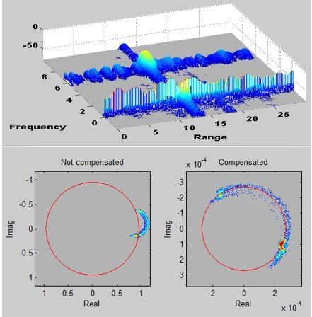The validity of such a model can be checked by plotting the locus of s(t) with time. We call this plot “Complex Scatter Plot” (CSP); examples taken from real data are shown in Figure 6. In the figure, the color represents the log count of the complex Radar returns after many minutes of observations (that corresponds to thousands of samples), superposed to the circle fitting the measures, as shown in Figure 5b. The fit is rather good is most cases, whereas in some cases data are better fitted by two or more circles, which is due to the variation of clutter with time. We will discuss this case in the next section.

The proposed clutter removal is carried out by first estimating the three parameters in Equation (14), carried out by the minimization of the L₁ norm of the error (chosen for robustness):

$$\widehat{{\rho }_I},\widehat{{\psi }_I},\widehat{A_T}=\arg \min {\displaystyle \sum }_n\left|\left|s\left(t_n\right)-{\rho }_I·\exp \left(j{\psi }_I\right)\right|-A_T\right|$$

(15)

and then retrieving the target contributions:

$${\widehat{s}}_T\left(t\right)=s\left(t\right)-\widehat{{\rho }_I}\exp \left(j\widehat{{\psi }_I}\right)$$

(16)

The minimization of Equation (18) is done numerically by systematically exploring the 2D space (${\rho }_I,{\psi }_I$) and, for each pair, by imposing:

$${\widehat{A}}_T=\frac{1}{N}{\displaystyle \sum }_n\left|\left|\mathit{s}\left(t_n\right)-{\rho }_I·\exp \left(j{\psi }_I\right)\right|\right|$$

(17)

The accuracy of the solution measures. The entity of the interference can be visualized in Figure 6 by the goodness of the fit between the black circle and the locus of the can be guessed by the amplitude of the center O’, that is, the length of |O−O’|: The larger it is, the stronger the interference. The signal to interference noise ratio can be computed by the ratio between the two radii:

$$SNIR={\left(\frac{A_T}{{\rho }_I}\right)}^2$$

(18)

Small Vibrations

The clutter removal method herein described relies on the identification of the circle fitting the loci of data amplitudes, |s(t)|, at different times. This can be done if the angle of s(t) varies appreciably, which occurs if the total deformation is a significant fraction of the wavelength, λ = 1.7 cm in the examples assumed so far.

However, for small vibrations, we can intentionally superpose some motion to the target to be measured, by means of a motorized target, like the one shown in Figure 7a. The motor introduces a harmonic vibration, which adds up to the deformation, causing a significant Doppler shift. The effect is quite evident in the power spectra plotted at a different range in Figure 7b, where the target can be easily identified by the ~6 Hz contribution at a ~12 m range. Within the same range, the complex amplitude measured at frequency corresponds to the clutter, which can be easily removed.

The effectiveness of the approach can be verified by observing the CSP diagrams before and after clutter removal, in Figure 7c,d. The harmonic motion of the target before and after the clutter compensation is shown in Figure 8. Please note that the full peak-to-peak vibration of 8 mm is reconstructed out of the 2 mm clutter-affected, while the spectral distortion is nulled.

This approach can also be exploited for separating the contribution of a slow-moving clutter. In this case, the signal model, in Equation (14), can be modified as follows:

$$s\left(t\right)={\rho }_I\exp \left(j{\psi }_I\left(t\right)\right)+A_T\exp \left(j\left(\omega t+{\psi }_T\left(t\right)\right)\right)$$

(19)

ω being the angular speed of the moving target. The result, s(t), is made of two contributions, the first being the interference—eventually time-varying—and the second the phase modulated signal. The latter is quite separable in the frequency domain from the first, provided that the spectra do not overlap, which can be checked using the analysis shown in Figure 7c.

5. Implementation and Validation

The proposed method to perform 2D/3D vibration estimation is summarized in the block diagram of Figure 9. The elements of the blocks are described in the previous sections: Note the use of the CSP to provide an evaluation of the possible interference, hence the target quality.

The method has been tested in laboratory with two Q band Radars, operating with about 800 MHz bandwidth, which allows for 20 cm resolution. The testbed for checking the 2D/3D vibration estimation is shown in Figure 10.

For the sake of simplicity, we used two Radars that were closely located just by stacking one upon the other. The 2D layout allowed us to measure only the displacements in the (x, z) plane, represented in Figure 10a.

A first set of measures was done by moving the target in the LOS x-axis, and a second set by moving the target in (x,y), along the 15° tilted basement shown in the figure. Results are shown in Figure 11.

In this experiment, the extent of a range resolution, 20 cm, marked by the red arrow in Figure 10a, was such that many reflections were superposed, in addition to that of the target itself. In fact, the CSP diagrams in Figure 11a, Figure 11c show a marked interference. Unless compensated, this would completely jeopardize the motion estimation, as shown on the top panel in Figure 11b. However, the compensation was capable of removing the bulk of the error, as shown in the bottom panel of the same figure. The method described in Equation (15) was good enough, since the total target displacement, 5 mm, was even larger that the wavelength.

The second case, the 15° tilted motion, was more complex, since the interference was changing over time, as one notices by the multiple circles in the CSP of Figure 11c. Therefore, the compensation was carried out by implementing Equation (15) in overlapped time-blocks. In this case, too, the method was effective in removing the clutter and retrieve the precise target displacement, as shown in Figure 11c.

6. Conclusions

The paper proposed a technique to estimate 2D or 3D vibrations by using two or three synchronized Radars and at least two fixed calibrators. The use of simple and cost-effective devices is the major advantage with respect to complex real or synthetic aperture or MIMO Radar. Methods to properly remove the distortion due to (a) propagation and Radar vibration and (b) interference from fixed targets were discussed, and results shown in both laboratories and a full-scale campaign.

The accuracy of a single Radar in estimating deformations has been estimated in terms of microns by comparison with accelerometers. The Radar has lower accuracy; however, it is still in the micron range, which is balanced by its sensitivity to the very slow components of the displacements. It has been shown that this accuracy worsens by a factor of three, in the worst case, in the estimation of 3D vibrations by three Radars closely spaced within 30°. An example of retrieving 2D millimetric displacements with very low errors has been shown in a controlled laboratory experiment.

It can be concluded that a Radar is complementary in respect of accelerometers, whereby the lower sensitivity is compensated by the remote measure form, the greater accuracy in the nearly static rates, and the simultaneous measures from multiple targets.

7. Patents

Part of the methods herein discussed are proposed in the patents:

• EP 2937711B1, “Method and system for the remote monitoring of the two/three-dimensional field of displacements and vibrations of items/structures” Eni S.p.A., granted 1 November 2017.
• EP 2937710A1” method and kinematic calibration system for measuring displacements and vibrations of items/structures” Eni S.p.A, granted 14 March 2018.