Evaluation of Sensor and Environmental Factors Impacting the Use of Multiple Sensor Data for Time-Series Applications
Abstract
:1. Introduction
2. Materials and Methods
2.1. Forest Canopy Model
2.2. Modeling Defoliation
2.3. Modeling the Signal for Different Data Products
2.3.1. TOA Reflectance Data
- is the planetary reflectance
- is the spectral radiance at the sensor’s aperture
- d is the earth-sun distance in astronomical units
- is the mean solar exoatmospheric irradiance
- is the solar zenith angle
2.3.2. Surface Refectance Derived Using ELM
- is the mean exoatmospheric irradiance
- is the reflectance factor of the Lambertian panel
- is the upwelled radiance
- is the downwelled radiance
- is the transmittance from the ground to the sensor
- is the solar zenith angle
2.3.3. Surface Refectance from Canopy BRDF
2.4. Factor Effects
2.4.1. RSR
- is the TOA reflectance for a specific spectral band
- is the effective BRDF reflectance (adjusted by the shape of the RSR)
- is the BRDF reflectance of the canopy
- n is the number of sun, view , and visibility combinations randomly selected
- k is the number of sun, view combinations shown in Table 1
2.4.2. Across-Track View Angle Effects
2.4.3. Visibility
2.4.4. Solar Zenith (SZN) Effect
3. Results and Discussion
3.1. Defoliated Forests
3.2. Modeling the Signal for Different Products
3.2.1. Radiance and Reflectance Products
3.2.2. NDVI Products
3.3. Factor Effect Analysis
3.3.1. RSR
3.3.2. Across-Track effect
3.3.3. Visibility Effects
3.3.4. SZN Effects
4. Conclusions
- The effect of atmospheric differences between two scenes due to changes in the visibility conditions can introduce as much effect as would be observed when the forest defoliates by 40%, but if compensated, the effect can be reduced to 1–7% in defoliation depending on the accuracy of the atmospheric compensation algorithm. The atmospheric attenuation is observed to be the most significant factor among all the factors considered in this study. Both the USGS (Landsat) and ESA (Sentinel-2) provide TOA products as their default/standard products, and as demonstrated in this study, if the atmosphere is not compensated, the effect of atmosphere can introduce large uncertainty in the estimation of forest defoliation.
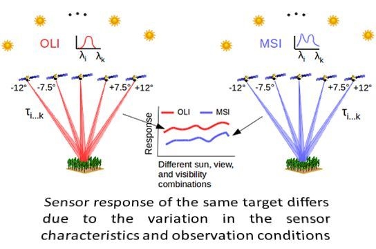
- The effect due to RSR differences between Landsat 8 and Sentinel 2 is observed to be 20% in defoliation, but compensation algorithm such as SBAF can reduce the effect to 1–7% in defoliation depending on whether the atmospheric attenuations are compensated or not.
- The cross-track view angle differences can introduce effects anywhere from 9% to 40% in defoliation depending on the accuracy of the atmospheric compensation algorithms.
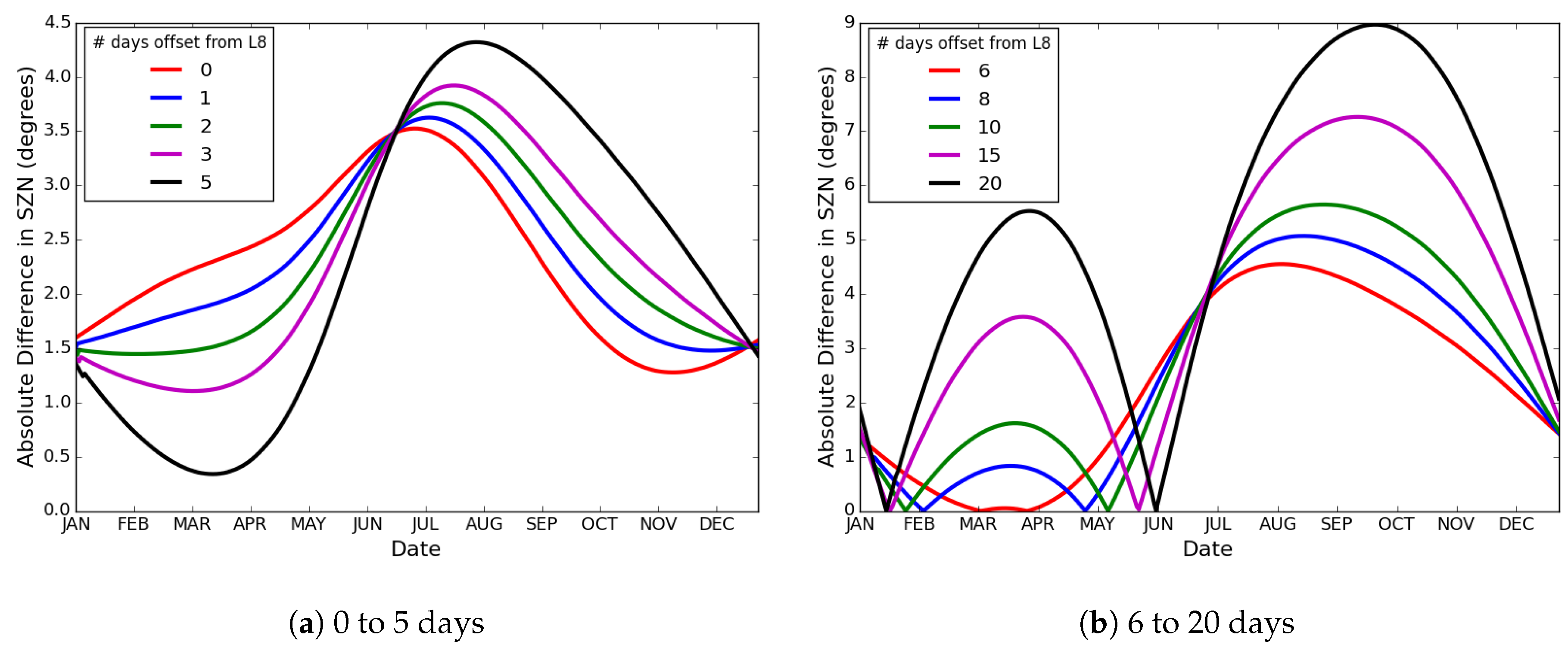
- For 5 days difference in acquisition between Landsat 8 and Sentinel 2 sensors, the effect of SZN angle differences can introduce effects ranging from 4% to 10% in defoliation depending on whether the atmospheric attenuations are compensated or not.
- Analysis of effects on the real data (OLI) acquired over a period of 23 days indicates that more than half the observed changes are likely to be due to the effects of the factors.
- Target specific and sensor specific SBAF values should be estimated and provided to the user community either using the real or simulated data. Many recent studies have used SBAF techniques to normalize for spectral response differences [44,45], but they were predominantly estimated using pseudo-invariant sites like desert sites for calibration purposes. Since SBAF values are both target and sensor specific, modeling approach as shown here for deciduous canopy can be used to estimate for other land cover classes.
- Understanding that the factors identified in this research can introduce real effects, future time series analysis should provide the uncertainty in their estimation that are based on the uncompensated and residual effects. Our study provides the first-order uncertainty estimates due to these factors, which can be used effectively to derive accuracy metrics in forest applications.
- Atmospheric compensation and compensation for sensor differences (RSR) should be applied for the data used in time-series applications. The Landsat and Sentinel-2 data providers have been providing surface reflectance data on-demand, but no associated uncertainty estimates are available for these products. The atmospheric compensation algorithm proposed by [46] and used in generating Landsat surface reflectance products indicate, that it is not uncommon to expect a 6% uncertainty in surface reflectance products using their algorithm. However, this is an overall estimate, and cannot be used as per-pixel uncertainty estimates for every data products. In the future, data providers should focus on per-pixel uncertainty estimates rather than a product or algorithm level uncertainty.
- Future research should focus on validating the accuracy of the atmospheric compensation algorithms used in generating the Landsat surface reflectance products using the real data if possible, or with the simulated data, and improve the algorithm as necessary. As shown in this study, atmospheric compensation has the potential to reduce the uncertainty in the products, but it has to be done correctly, as otherwise, it increases the uncertainty. This is one reason future research should focus on validating the surface reflectance products.
Author Contributions
Funding
Acknowledgments
Conflicts of Interest
References
- Markham, B.L.; Helder, D.L. Forty-year calibrated record of earth-reflected radiance from Landsat: A review. Remote Sens. Environ. 2012, 122, 30–40. [Google Scholar] [CrossRef] [Green Version]
- Schott, J.R.; Gerace, A.D.; Brown, S.D.; Gartley, M.G. Modeling the image performance of the Landsat Data Continuity Mission sensors. In Proceedings of the SPIE Optical Engineering+ Applications, San Diego, CA, USA, 21–25 August 2011; p. 81530F. [Google Scholar]
- Storey, J.C. Landsat 7 on-orbit modulation transfer function estimation. In Proceedings of the International Symposium on Remote Sensing, Toulouse, France, 17–21 September 2001; pp. 50–61. [Google Scholar]
- Masek, J.G.; Vermote, E.F.; Saleous, N.E.; Wolfe, R.; Hall, F.G.; Huemmrich, K.F.; Gao, F.; Kutler, J.; Lim, T.K. A Landsat surface reflectance dataset for North America, 1990–2000. IEEE Geosci. Remote Sens. Lett. 2006, 3, 68–72. [Google Scholar] [CrossRef]
- Tan, B.; Morisette, J.T.; Wolfe, R.E.; Gao, F.; Ederer, G.A.; Nightingale, J.; Pedelty, J.A. An Enhanced TIMESAT Algorithm for Estimating Vegetation Phenology Metrics From MODIS Data. IEEE J. Sel. Top. Appl. Earth Obs. Remote Sens. 2011, 2, 361–371. [Google Scholar] [CrossRef]
- Mishra, N.; Haque, M.O.; Leigh, L.; Aaron, D.; Helder, D.; Markham, B. Radiometric Cross Calibration of Landsat 8 Operational Land Imager (OLI) and Landsat 7 Enhanced Thematic Mapper Plus (ETM+). Remote Sens. 2014, 6, 12619–12638. [Google Scholar] [CrossRef] [Green Version]
- Chander, G.; Meyer, D.J.; Helder, D.L. Cross calibration of the Landsat-7 ETM+ and EO-1 ALI sensor. IEEE Trans. Geosci. Remote Sens. 2004, 42, 2821–2831. [Google Scholar] [CrossRef]
- Zhang, H.K.; Roy, D.P.; Yan, L.; Li, Z.; Huang, H.; Vermote, E.; Skakun, S.; Roger, J.C. Characterization of Sentinel-2A and Landsat-8 top of atmosphere, surface, and nadir BRDF adjusted reflectance and NDVI differences. Remote Sens. Environ. 2018, 215, 482–494. [Google Scholar] [CrossRef]
- Mandanici, E.; Bitelli, G. Preliminary Comparison of Sentinel-2 and Landsat 8 Imagery for a Combined Use. Remote Sens. 2016, 8, 1014. [Google Scholar] [CrossRef]
- Gorroño, J.; Banks, A.C.; Fox, N.P.; Underwood, C. Radiometric inter-sensor cross-calibration uncertainty using a traceable high accuracy reference hyperspectral imager. ISPRS J. Photogramm. Remote Sens. 2017, 130, 393–417. [Google Scholar] [CrossRef]
- Chen, C.P.; Zhang, C.Y. Data-intensive applications, challenges, techniques and technologies: A survey on Big Data. Inform. Sci. 2014, 275, 314–347. [Google Scholar] [CrossRef]
- Liu, P.; Di, L.; Du, Q.; Wang, L. Remote Sensing Big Data: Theory, Methods and Applications. Remote Sens. 2018, 10, 711. [Google Scholar] [CrossRef]
- Rengarajan, R.; Schott, J.R. Modeling and Simulation of Deciduous Forest Canopy and Its Anisotropic Reflectance Properties Using the Digital Image and Remote Sensing Image Generation (DIRSIG) Tool. IEEE J. Sel. Top. Appl. Earth Obs. Remote Sens. 2017, 10, 4805–4817. [Google Scholar] [CrossRef]
- Rengarajan, R. Evaluation of Sensor, Environment and Operational Factors Impacting the Use of Multiple Sensor Constellations for Long Term Resource Monitoring. Ph.D. Thesis, Rochester Institute of Technology, Rochester, NY, USA, 2016. [Google Scholar]
- Yao, T.; Yang, X.; Zhao, F.; Wang, Z.; Zhang, Q.; Jupp, D.; Lovell, J.; Culvenor, D.; Newnham, G.; Ni-Meister, W.; et al. Measuring forest structure and biomass in New England forest stands using Echidna ground-based lidar. Remote Sens. Environ. 2011, 115, 2965–2974. [Google Scholar] [CrossRef]
- Yang, X.; Tang, J.; Mustard, J.F.; Wu, J.; Zhao, K.; Serbin, S.; Lee, J.E. Seasonal variability of multiple leaf traits captured by leaf spectroscopy at two temperate deciduous forests. Remote Sens. Environ. 2016, 179, 1–12. [Google Scholar] [CrossRef] [Green Version]
- Brown, S.D.; Schott, J.R. Verification and Validation Studies of the DIRSIG Data Simulation Model; Technical Report 1; Rochester Institute of Technology: Rochester, NY, USA, 2010. [Google Scholar]
- Brown, S.D.; Goodenough, A.A. DIRSIG Documentation Manual; Technical Report; Rochester Institute of Technology: Rochester, NY, USA, 2015. [Google Scholar]
- Goodenough, A.A.; Brown, S.D. Development of land surface reflectance models based on multiscale simulation. In Proceedings of the SPIE Algorithms and Technologies for Multispectral, Hyperspectral, and Ultraspectral Imagery XXI, Baltimore, MD, USA, 20–24 April 2015; Volume 9472, p. 94720D. [Google Scholar]
- Widlowski, J.L.; Côté, J.F.; Béland, M. Abstract tree crowns in 3D radiative transfer models: Impact on simulated open-canopy reflectances. Remote Sens. Environ. 2014, 142, 155–175. [Google Scholar] [CrossRef]
- Spruce, J.P.; Sader, S.; Ryan, R.E.; Smoot, J.; Kuper, P.; Ross, K.; Prados, D.; Russell, J.; Gasser, G.; McKellip, R.; et al. Assessment of MODIS NDVI time series data products for detecting forest defoliation by gypsy moth outbreaks. Remote Sens. Environ. 2011, 115, 427–437. [Google Scholar] [CrossRef]
- De Beurs, K.M.; Townsend, P.A. Estimating the effect of gypsy moth defoliation using MODIS. Remote Sens. Environ. 2008, 112, 3983–3990. [Google Scholar] [CrossRef]
- Onyx Computing. Onyx Tree. 2015. Available online: http://www.onyxtree.com (accessed on 23 October 2018).
- Frederic Baret. PROSPECT Inversion. 2015. Available online: http://teledetection.ipgp.jussieu.fr/prosail/ (accessed on 23 October 2018).
- Feret, J.B.; François, C.; Asner, G.P.; Gitelson, A.A.; Martin, R.E.; Bidel, L.P.; Ustin, S.L.; le Maire, G.; Jacquemoud, S. PROSPECT-4 and 5: Advances in the leaf optical properties model separating photosynthetic pigments. Remote Sens. Environ. 2008, 112, 3030–3043. [Google Scholar] [CrossRef]
- Lucht, W.; Schaaf, C.B.; Strahler, A.H. An algorithm for the retrieval of albedo from space using semiempirical BRDF models. IEEE Trans. Geosci. Remote Sens. 2000, 38, 977–998. [Google Scholar] [CrossRef]
- Schaaf, C.B.; Gao, F.; Strahler, A.H.; Lucht, W.; Li, X.; Tsang, T.; Strugnell, N.C.; Zhang, X.; Jin, Y.; Muller, J.P.; et al. First operational BRDF, albedo nadir reflectance products from MODIS. Remote Sens. Environ. 2002, 83, 135–148. [Google Scholar] [CrossRef] [Green Version]
- McManus, M.; Schneeberger, N.; Reardon, R.; Mason, G. Gypsy Moth. USDA Forest Service Forest Insect and Disease Leaflet 162; 1989. Available online: https://www.fs.usda.gov/Internet/FSE_DOCUMENTS/fsbdev2_043394.pdf (accessed on 23 October 2018).
- Tree Diseases. Trees and Shrubs: Diseases, Insects and Other Problems. 2016. Available online: https://extension.umn.edu/tree-selection-and-care/forest-pests-and-diseases#insects-1270960 (accessed on 23 October 2018).
- Wanner, W.; Li, X.; Strahler, A.H. On the derivation of kernels for kernel-driven models of bidirectional reflectance. J. Geophys. Res. Atmos. 1995, 100, 21077–21089. [Google Scholar] [CrossRef]
- Anderson, G.P.; Berk, A.; Acharya, P.K.; Matthew, M.W.; Bernstein, L.S.; Chetwynd, J.H., Jr.; Dothe, H.; Adler-Golden, S.M.; Ratkowski, A.J.; Felde, G.W.; et al. MODTRAN4: Radiative transfer modeling for remote sensing. In Proceedings of the SPIE Optics in Atmospheric Propagation and Adaptive Systems III, Florence, Italy, 20–24 September 1999; Volume 3866, pp. 2–10. [Google Scholar]
- NASA Goddard Space Flight Center. Landsat 7 Science Data Users Handbook; Landsat Project Science Office, NASA Goddard Space Flight Center: Greenbelt, MD, USA, 2009.
- Schott, J.R. Remote Sensing: The Image Chain Approach; Oxford University Press: New York, NY, USA, 2007. [Google Scholar]
- Li, S.; Ganguly, S.; Dungan, J.L.; Wang, W.; Nemani, R.R. Sentinel-2 MSI radiometric characterization and cross-calibration with Landsat-8 OLI. Adv. Remote Sens 2017, 6, 147. [Google Scholar] [CrossRef]
- Pahlevan, N.; Smith, B.; Binding, C.; O’Donnell, D. Spectral band adjustments for remote sensing reflectance spectra in coastal/inland waters. Opt. Express 2017, 25, 28650–28667. [Google Scholar] [CrossRef]
- Morfitt, R.; Barsi, J.; Levy, R.; Markham, B.; Micijevic, E.; Ong, L.; Scaramuzza, P.; Vanderwerff, K. Landsat-8 Operational Land Imager (OLI) Radiometric Performance On-Orbit. Remote Sens. 2015, 7, 2208–2237. [Google Scholar] [CrossRef] [Green Version]
- Drusch, M.; Del Bello, U.; Carlier, S.; Colin, O.; Fernandez, V.; Gascon, F.; Hoersch, B.; Isola, C.; Laberinti, P.; Martimort, P.; et al. Sentinel-2: ESA’s Optical High-Resolution Mission for GMES Operational Services. Remote Sens. Environ. 2012, 120, 25–36. [Google Scholar] [CrossRef]
- ESA. Sentinel-2 Spectral Response Functions (S2-SRF). 2017. Available online: https://earth.esa.int/web/sentinel/user-guides/sentinel-2-msi/document-library (accessed on 23 October 2018).
- Chander, G.; Mishra, N.; Helder, D.L.; Aaron, D.B.; Angal, A.; Choi, T.; Xiong, X.; Doelling, D.R. Applications of Spectral Band Adjustment Factors (SBAF) for Cross-Calibration. IEEE Trans. Geosci. Remote Sens. 2013, 51, 1267–1281. [Google Scholar] [CrossRef]
- Teillet, P.M.; Markham, B.L.; Irish, R.R. Landsat cross-calibration based on near simultaneous imaging of common ground targets. Remote Sens. Environ. 2006, 102, 264–270. [Google Scholar] [CrossRef] [Green Version]
- Teillet, P.M.; Barker, J.L.; Markham, B.L.; Irish, R.R.; Fedosejevs, G.; Storey, J.C. Radiometric cross-calibration of the Landsat-7 ETM+ and Landsat-5 TM sensors based on tandem data sets. Remote Sens. Environ. 2001, 78, 39–54. [Google Scholar] [CrossRef] [Green Version]
- Czapla-Myers, J.; McCorkel, J.; Anderson, N.; Thome, K.; Biggar, S.; Helder, D.; Aaron, D.; Leigh, L.; Mishra, N. The Ground-Based Absolute Radiometric Calibration of Landsat 8 OLI. Remote Sens. 2015, 7, 600–626. [Google Scholar] [CrossRef] [Green Version]
- Wang, Q.; Adiku, S.; Tenhunen, J.; Granier, A. On the relationship of NDVI with leaf area index in a deciduous forest site. Remote Sens. Environ. 2005, 94, 244–255. [Google Scholar] [CrossRef]
- Mishra, N.; Helder, D.; Angal, A.; Choi, J.; Xiong, X. Absolute calibration of optical satellite sensors using Libya 4 pseudo invariant calibration site. Remote Sens. 2014, 6, 1327–1346. [Google Scholar] [CrossRef]
- Bouvet, M. Radiometric comparison of multispectral imagers over a pseudo-invariant calibration site using a reference radiometric model. Remote Sens. Environ. 2014, 140, 141–154. [Google Scholar] [CrossRef]
- Vermote, E.; Justice, C.; Claverie, M.; Franch, B. Preliminary analysis of the performance of the Landsat 8/OLI land surface reflectance product. Remote Sens. Environ. 2016, 185, 46–56. [Google Scholar] [CrossRef]


| Sun Angles | Defoliation | X-Track | Visibility | RSR | Spectral | |
|---|---|---|---|---|---|---|
| Zenith | Azimuth | Levels | Angles (deg) | (KM) | Bands | |
| 35 | 145 | 0% | −12 | 10 | OLI (L8) | RED |
| 30 | 137 | 10% | −7.5 | 15 | MSI (S2A) | NIR |
| 33 | 157 | 20% | 0 | 20 | ||
| 25 | 150 | 25% | 7.5 | 25 | ||
| 27 | 135 | 30% | 12 | |||
| 35 | 165 | 40% | ||||
| 20 | 150 | 55% | ||||
| 23 | 132 | 70% | ||||
| 40 | 150 | 85% | ||||
| 38 | 153 | |||||
| Level of Defoliation | Data Products in the Red Spectral Band | ||||
|---|---|---|---|---|---|
| TOA RAD μ (σ) | TOA REFL μ (σ) | ELM-Typical μ (σ) | ELM-Ideal μ (σ) | BRF μ (σ) | |
| 0% | 0 (0) | 0 (0) | 0 (0) | 0 (0) | 0 (0) |
| 10% | 0.25 (0.09) | 0.25 (0.09) | 1.32 (0.54) | 1.36 (0.48) | 1.05 (0.44) |
| 20% | 0.59 (0.19) | 0.59 (0.19) | 3.07 (1.05) | 3.17 (0.93) | 2.36 (0.86) |
| 25% | 0.75 (0.23) | 0.75 (0.23) | 3.85 (1.19) | 3.98 (1.04) | 3.25 (1.03) |
| 30% | 1.02 (0.31) | 1.02 (0.31) | 5.26 (1.54) | 5.45 (1.35) | 4.52 (1.36) |
| 40% | 1.64 (0.46) | 1.64 (0.46) | 8.40 (2.19) | 8.71 (1.84) | 7.55 (1.79) |
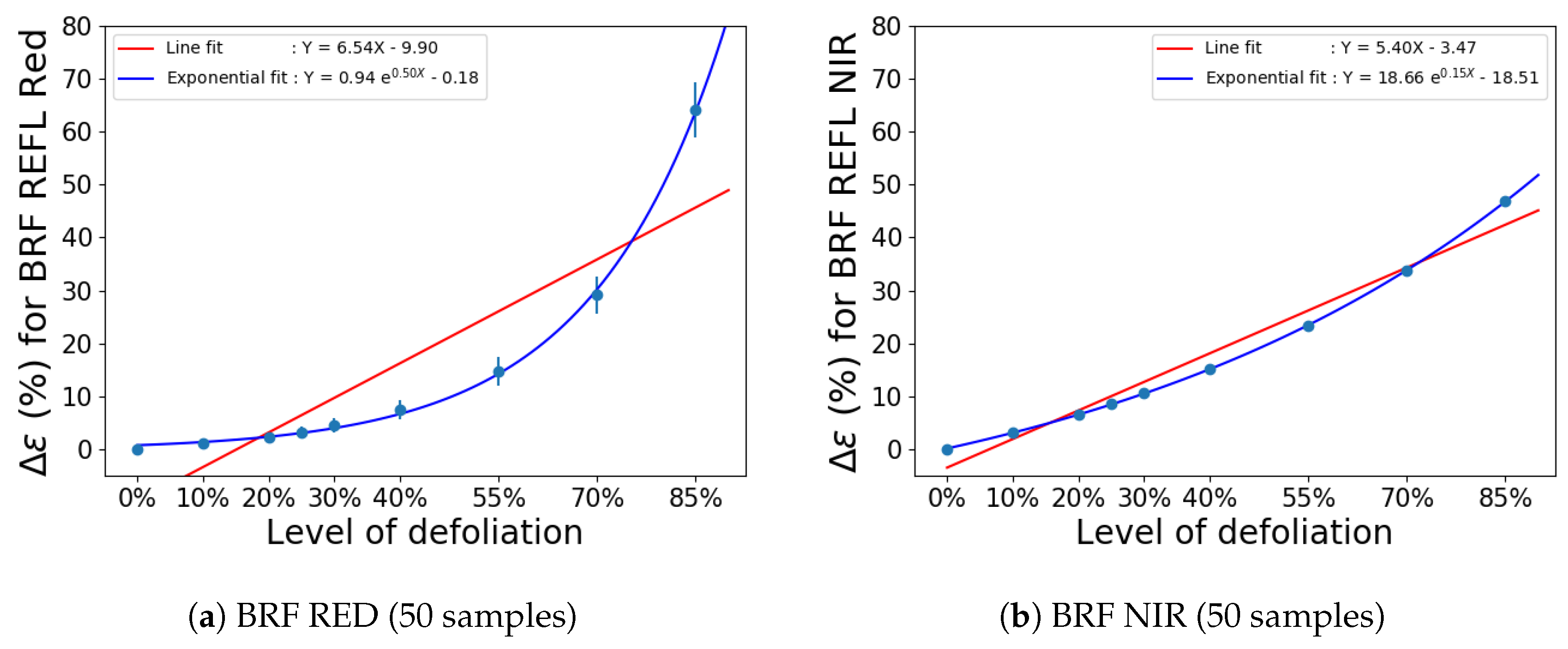
| 55% | 3.11 (0.83) | 3.11 (0.83) | 15.86 (3.57) | 16.44 (2.69) | 14.73 (2.61) |
| 70% | 6.00 (1.56) | 6.00 (1.56) | 30.40 (6.02) | 31.52 (3.99) | 29.16 (3.51) |
| 85% | 12.86 (3.42) | 12.86 (3.42) | 64.80 (11.84) | 67.21 (6.90) | 64.15 (5.21) |
| Level of Defoliation | Data Products in the Red Spectral Band | ||||
|---|---|---|---|---|---|
| TOA RAD μ (σ) | TOA REFL μ (σ) | ELM-Typical μ (σ) | ELM-Ideal μ (σ) | BRF μ (σ) | |
| 0% | 0 (0) | 0 (0) | 0 (0) | 0 (0) | 0 (0) |
| 10% | 2.39 (0.31) | 2.39 (0.31) | 2.95 (0.30) | 2.96 (0.30) | 3.18 (0.18) |
| 20% | 5.14 (0.48) | 5.14 (0.48) | 6.34 (0.34) | 6.36 (0.35) | 6.63 (0.29) |
| 25% | 6.70 (0.55) | 6.70 (0.55) | 8.27 (0.31) | 8.29 (0.32) | 8.54 (0.34) |
| 30% | 8.37 (0.70) | 8.37 (0.70) | 10.33 (0.45) | 10.36 (0.46) | 10.61 (0.42) |
| 40% | 11.97 (0.92) | 11.97 (0.92) | 14.78 (0.44) | 14.78 (0.44) | 15.18 (0.46) |
| 55% | 18.47 (1.36) | 18.47 (1.36) | 22.81 (0.55) | 22.81 (0.57) | 23.32 (0.54) |
| 70% | 27.07 (1.83) | 27.07 (1.83) | 33.44 (0.43) | 33.53 (0.45) | 33.81 (0.47) |
| 85% | 37.86 (2.45) | 37.86 (2.45) | 46.76 (0.28) | 46.90 (0.33) | 46.86 (0.37) |
| Level of Defoliation | NDVI Products | ||||
|---|---|---|---|---|---|
| TOA RAD μ (σ) | TOA REFL μ (σ) | ELM-Typical μ (σ) | ELM-Ideal μ (σ) | BRF μ (σ) | |
| 0% | 0 (0) | 0 (0) | 0 (0) | 0 (0) | 0 (0) |
| 10% | 1.30 (0.16) | 0.85 (0.10) | 0.38 (0.04) | 0.37 (0.03) | 0.37 (0.01) |
| 20% | 2.89 (0.30) | 1.89 (0.18) | 0.87 (0.08) | 0.84 (0.04) | 0.82 (0.03) |
| 25% | 3.80 (0.38) | 2.50 (0.22) | 1.14 (0.10) | 1.10 (0.04) | 1.100 (0.03) |
| 30% | 4.86 (0.47) | 3.19 (0.27) | 1.50 (0.12) | 1.45 (0.05) | 1.44 (0.04) |
| 40% | 7.26 (0.65) | 4.78 (0.37) | 2.33 (0.17) | 2.26 (0.07) | 2.27 (0.05) |
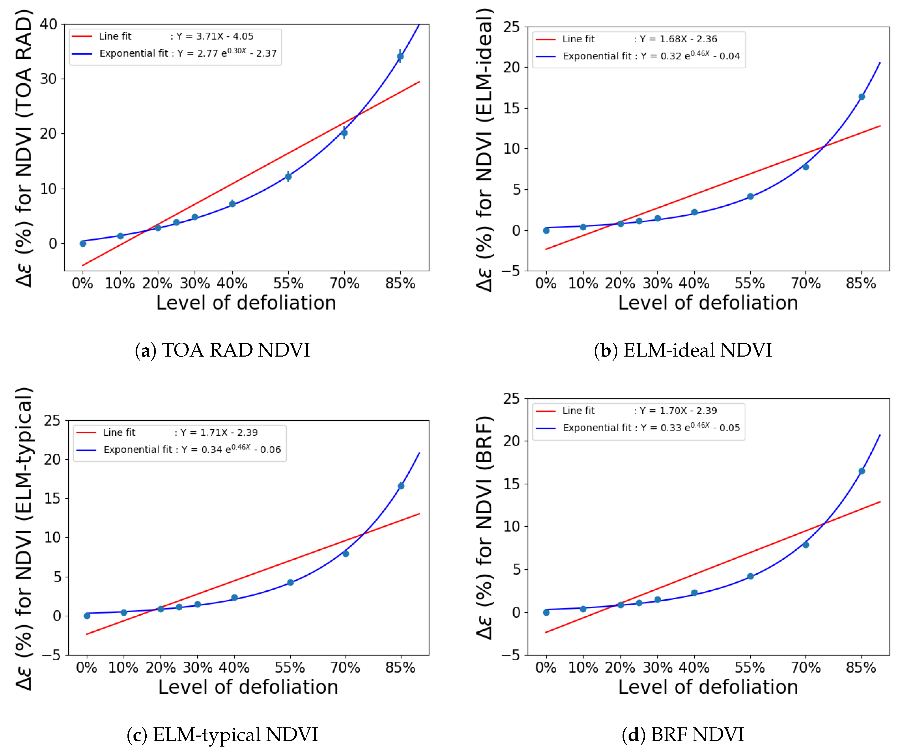
| 55% | 12.18 (0.94) | 8.06 (0.53) | 4.25 (0.26) | 4.14 (0.08) | 4.17 (0.07) |
| 70% | 20.16 (1.26) | 13.47 (0.69) | 7.97 (0.38) | 7.80 (0.10) | 7.85 (0.10) |
| 85% | 34.07 (1.27) | 23.14 (0.60) | 16.63 (0.50) | 16.39 (0.27) | 16.51 (0.21) |
| Data | RED | NIR | NDVI |
|---|---|---|---|
| Products | Relative Error | Relative Error | Relative Error |
| TOA Rad | 6.1% | 1.5% | 6.9% |
| TOA Refl | 6.1% | 1.5% | 7.4% |
| ELM-typical Refl | 6.3% | 1.5% | 10.9% |
| ELM-ideal Refl | 6.2% | 1.5% | 10.9% |
| BRF Refl | 5.3% | 0.9% | 10.6% |
| Data | Uncompensated | SBAF (TOA REFL) | SBAF (BRF) |
|---|---|---|---|
| Products | Mean (STD) | Mean (STD) | Mean (STD) |
| NDVI TOA Rad | 19% (2.2%) | 2% (1.3%) | 7% (3.4%) |
| NDVI TOA Refl | 19% (1.9%) | 2% (1.3%) | 7% (3.2%) |
| NDVI ELM-typical Refl | 15% (1.5%) | 3% (0.6%) | 1% (0.9%) |
| NDVI ELM-ideal Refl | 15% (0.8%) | 3% (0.5%) | 1% (0.5%) |
| Data | Uncompensated | SBAF (TOA REFL) | SBAF (BRF) |
|---|---|---|---|
| Products | Mean (STD) | Mean (STD) | Mean (STD) |
| NDVI TOA Rad | 17% (8.8%) | 8% (5.7%) | 11% (8.2%) |
| NDVI TOA Refl | 17% (8.6%) | 8% (5.7%) | 10% (8.1%) |
| NDVI ELM-typical Refl | 28% (21.5%) | 28% (21.3%) | 28% (21.9%) |
| NDVI ELM-ideal Refl | 16% (5.0%) | 5% (3.8%) | 4% (2.7%) |
| NDVI BRF Refl | 5% (2.8%) | 5% (2.8%) | 5% (2.8%) |
| Data | Uncompensated | SBAF (TOA REFL) | SBAF (BRF) |
|---|---|---|---|
| Products | Mean (STD) | Mean (STD) | Mean (STD) |
| NDVI TOA Rad | 14% (4.6%) | 14% (4.7%) | 14% (4.8%) |
| NDVI TOA Refl | 14% (4.5%) | 14% (4.7%) | 14% (4.7%) |
| NDVI ELM-typical Refl | 40% (21.7%) | 40% (22.1%) | 40% (22.2%) |
| NDVI ELM-ideal Refl | 9% (2.6%) | 9% (3.8%) | 9% (2.7%) |
| NDVI BRF Refl | 10% (3.2%) | 10% (3.2%) | 10% (3.2%) |
| Data | Uncompensated | SBAF (TOA REFL) | SBAF (BRF) |
|---|---|---|---|
| Products | Mean (STD) | Mean (STD) | Mean (STD) |
| NDVI TOA Rad | 40% (39%) | 40% (40%) | 40% (39%) |
| NDVI TOA Refl | 40% (38%) | 40% (39%) | 40% (38%) |
| NDVI ELM-typical Refl | 16% (10%) | 8% (9%) | 7% (9.7%) |
| NDVI ELM-ideal Refl | 15% (1.4%) | 4% (1.3%) | 1% (0.9%) |
| Data | Uncompensated | SBAF (TOA REFL) | SBAF (BRF) |
|---|---|---|---|
| Products | Mean (STD) | Mean (STD) | Mean (STD) |
| NDVI TOA Rad | 10% (5%) | 10% (5%) | 10% (5%) |
| NDVI TOA Refl | 10% (5%) | 10% (5%) | 10% (5%) |
| NDVI ELM-typical Refl | 8% (7%) | 8% (7%) | 8% (7%) |
| NDVI ELM-ideal Refl | 4% (1.4%) | 4% (1.4%) | 4% (1.4%) |
| NDVI BRF | 4% (1.6%) | 4% (1.6%) | 4% (1.6%) |
© 2018 by the authors. Licensee MDPI, Basel, Switzerland. This article is an open access article distributed under the terms and conditions of the Creative Commons Attribution (CC BY) license (http://creativecommons.org/licenses/by/4.0/).
Share and Cite
Rengarajan, R.; Schott, J.R. Evaluation of Sensor and Environmental Factors Impacting the Use of Multiple Sensor Data for Time-Series Applications. Remote Sens. 2018, 10, 1678. https://doi.org/10.3390/rs10111678
Rengarajan R, Schott JR. Evaluation of Sensor and Environmental Factors Impacting the Use of Multiple Sensor Data for Time-Series Applications. Remote Sensing. 2018; 10(11):1678. https://doi.org/10.3390/rs10111678
Chicago/Turabian StyleRengarajan, Rajagopalan, and John R. Schott. 2018. "Evaluation of Sensor and Environmental Factors Impacting the Use of Multiple Sensor Data for Time-Series Applications" Remote Sensing 10, no. 11: 1678. https://doi.org/10.3390/rs10111678
APA StyleRengarajan, R., & Schott, J. R. (2018). Evaluation of Sensor and Environmental Factors Impacting the Use of Multiple Sensor Data for Time-Series Applications. Remote Sensing, 10(11), 1678. https://doi.org/10.3390/rs10111678


