Forest Cover and Vegetation Degradation Detection in the Kavango Zambezi Transfrontier Conservation Area Using BFAST Monitor

Abstract

Forest cover and vegetation degradation was monitored across the Kavango-Zambezi Transfrontier Conservation Area (KAZA) in southern Africa and the performance of three different methods in detecting degradation was assessed using reference data. Breaks for Additive Season and Trend (BFAST) Monitor was used to identify potential forest cover and vegetation degradation using Landsat Normalized Difference Moisture Index (NDMI) time series data. Parametric probability-based magnitude thresholds, non-parametric random forest in conjunction with Soil-Adjusted Vegetation Index (SAVI) time series, and the combination of both methods were evaluated for their suitability to detect degradation for six land cover classes ranging from closed canopy forest to open grassland. The performance of degradation detection was largely dependent on tree cover and vegetation density. Satisfactory accuracies were obtained for closed woodland (user’s accuracy 87%, producer’s accuracy 71%) and closed forest (user’s accuracy 92%, producer’s accuracy 90%), with lower accuracies for open canopies. The performance of the three methods was more similar for closed canopies and differed for land cover classes with open canopies. Highest user’s accuracy was achieved when methods were combined, and the best performance for producer’s accuracy was obtained when random forest was used.

1. Introduction

The Kavango-Zambezi Transfrontier Conservation Area (KAZA) is the largest transboundary conservation area in Africa, straddling the borders of Angola, Botswana, Namibia, Zambia and Zimbabwe (Figure 1). Changes in climate regimes and increased human activities which are driving increases in human-wildlife conflicts (HWC). Between 2007 and 2014, large animal herds changed their movement patterns for several reasons, increasing chances of HWC within KAZA [1], and related economic losses have been incurred, further fueling the spiral of HWC [2]. When animal movement patterns and human-induced land change are known, wildlife corridors can be planned and managed as a suitable solution to manage conflicts [3]. Such efforts are equally important for nations in slowing down forest decline and conserving or increasing carbon sink capacities of forests, promoted by Reducing Emissions from Deforestation and forest Degradation (REDD+) projects [4]. Monitoring, Reporting and Verification (MRV) of activity data [5] has been proven to create additional revenues when properly implemented [6], providing operational financial alternatives to land use change and reducing reliance on more exploitative activities [7].

To observe land cover change, bi-temporal remote sensing-based measurements of human-induced land change has been used previously in KAZA [8]. In particular, the Caprivi strip shows an ongoing human expansion of cropland and settlements and a transformation of closed woodland into secondary woods and shrub lands [9]. A long-term study from 1975–2014 used decadal remote sensing data, observing an acceleration of such trends [10]. Ecosystems were found to be impacted by an abundance of factors, such as the El Niño–Southern Oscillation [11], large-scale burning [12], and flooding events [13]. In comparison to other ecosystems, uncertainties of remote sensing-based measurements in savannah land cover types were particularly high [14]. Isolation of ecosystem variability from anthropogenic degradation was achieved using high-temporal resolution coarse-spatial resolution time series for small areas [15]. Other large-scale applications on continental or national scales have been achieved using sample-based approaches [16,17,18]. For KAZA, no large-scale study exists providing spatially explicit and up-to-date land degradation to meet the needs of mapping and reporting practices [19]. Long-term consistent observations have been used to measure global changes in tree cover, but these studies more often focus on dense forest and tend to exclude or omit detection in savannah landscapes, dry forests or bushlands which are most common in KAZA [20,21].

Breaks For Additive Season and Trend (BFAST) [22] type models have been used to measure forest decline across the tropics [23,24,25,26], but in contrast to [21], application has remained focused on local scales, similar to radio detection and ranging (RADAR) and optical time series fusion approaches [27,28]. The more popular BFAST Monitor (BFM) [29] applications have been found to be used robustly with different data sources [30]. BFM has been applied to describe patterns of anthropogenic forest change [31], for reconstructing land use history [32] and observing regrowth dynamics after degradation [33]. It has also been used in combination with community-based monitoring [25], for long-term studies [34], and also to map vegetation decline in arid and semi-arid environments [35,36]. The most common data source used is Landsat satellites, where BFM results are often post-processed using the so-called magnitude of change. Potential changes have been identified using either a threshold approach [26] or a random forest machine learning algorithm [37] to classify magnitude values [24,25,38]. Using BFM, multiple forest types have been studied regarding their biomass and changes, mostly excluding sparsely vegetated areas [39]. Only few BFM studies exist which apply accurate estimation of changes [19], including reporting accuracy confidences [40], besides existing consolidated standard measures [41], as they require exhaustive reference data. To date, no large-scale application of BFM exists observing vegetation degradation for a range of open- and closed-canopy, dry and moist ecosystems.

KAZA is characterized by a gradient of vegetation cover ranging from closed woodlands in the northern regions to open grasslands in the south. The main objective of this study was to assess the performance difference in degradation detection for six different classes in KAZA using BFM. We studied the performance of degradation detection using BFM for different canopy cover types, using modifications of existing methods [24,26], accounting for good practices and introducing a new method to refine results. Studies within similar setups [24,26,42,43] used the normalized difference moisture index (NDMI) [44] or the soil adjusted vegetation index (SAVI) [45]. The aforementioned accuracies were generally moderate, ranging approximately around 70–80%, but mostly lacked comprehensive reporting and did not split observed land into specific land cover classes. Particularly, commission of change was identified as a large error source for BFM applications [23]. We combined the advantages of existing non-parametric random forest-based methods [24], field data time series fusions [38,43] and conservative parametric magnitude threshold-based approaches [26] to identify the suitability of BFM to detect land cover degradation. The main objective of this study was to assess the performance difference in degradation detection for six different classes in KAZA using BFM. In this respect, post-processing of threshold-based and random forest-based BFM were compared in terms of the accuracy of detecting degradation. Finally, the effectiveness of combining both threshold-based and random forest-based BFM post-processing methods was studied.

Three research questions were addressed:

How does degradation detection performance differ for six different land cover classes in KAZA using BFM?

How does threshold-based and random forest-based BFM post-processing for degradation detection compare?

How are method variations impacting degradation detection accuracy and how can threshold-based and random forest-based BFM post-processing methods be effectively combined?

2. Methods

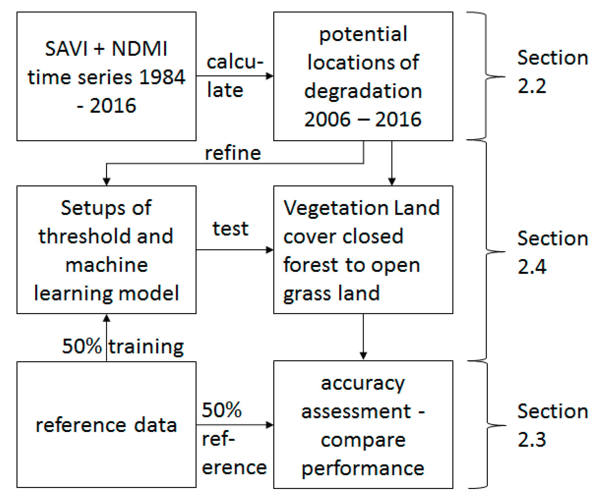
Figure 2 provides an outline of the current study. A description of the study area and relevant land cover classes subjected to degradation detection are provided in Section 2.1. Landsat-derived NDMI and SAVI data from the United States Geological Survey (USGS) were used for the degradation detection, because their combination has shown accurate results previously in similar environments [24]. Data pre-processing, time series construction and time series analysis are presented in Section 2.2. This includes statistical tests of the SAVI and NDMI time series for the occurrence of significant signal drops from 2006–2016 compared to 1984–2005 observations using BFM. In contrast, vegetation changes caused only by seasonality were considered to be stable vegetation (no change) [29]. Section 2.3 describes reference data used for accuracy assessment and for method calibration. Part of the reference data was used for a threshold-based approach [26], a random forest feature level fusion-based approach [24], and their combination to understand BFM suitability for the detection of land cover-specific degradations (Section 2.4).

The formula for the SAVI is provided below as Equation (1), which is a ratio of near-infrared (NIR) (NIR, TM (0.76–0.90 μm), ETM+ (0.77–0.90 μm)) and red (RED, TM/ETM+ (0.63–0.69 μm)). Similar to the normalized difference vegetation index (NDVI). The soil correction is expressed with a variable L, for which we select 0.5 [45,46].

$$SAVI=\left(1+L\right)\ast \left(\frac{\left(NIR-RED\right)}{\left(NIR+RED+L\right)}\right)$$

(1)

The formula of the NDMI is provided below as Equation (2), which is a ratio of NIR and short-wave infrared (SWIR1) (SWIR1, TM/ETM+ (1.55–1.75 μm)). The NDMI has proven to be an accurate tool when monitoring forests in the tropics [47].

$$NDMI=\frac{\left(NIR-SWIR1\right)}{\left(NIR+SWIR1\right)}$$

(2)

2.1. Study Area

KAZA comprises mixed savannah and dry forest landscapes with large grassland ranges, the world’s largest inland delta and dense bushlands and forested areas with a highly varying vegetation canopy (Figure 1). Tree cover increases from south to north. In addition to the effects of human activities, land cover is impacted by varying dry and wet seasons, and responses in spectral reflectance factors vary throughout the year. The near-infrared (NIR) and shortwave infrared (SWIR) bands are especially sensitive to these variations, as foliage disappears in the dry season and reoccurs again in the wet season. Land cover in 2005 was identified from existing products [13,48], and the identification of natural vegetated areas at 30 m resolution for the year 2005 [48] was used as a benchmark map. We updated the locations of wetlands using global surface water data [13] and applied a minimum mapping unit of 0.5 ha for all land cover types subjected to the degradation analysis.

Table 1. Classes and their definition, classes 1–6 were subjected to anthropogenic degradation detection [13,48].

Class Name	Description
no data	Absence of data
CW—closed canopy woodland	predominantly tree and herbaceous strata, where tree cover may be greater than 70%
CF—closed canopy forest	multiple vegetation strata likely, where tree cover is likely to be greater than 70%
CB—closed canopy bushland, thicket	closed–medium canopy short bushland and/or thicket areas multiple vegetation strata likely, where shrub and bush cover is likely to be greater than 70%
OW—open canopy woodland	Open canopy woodland and/or bushland, where the tree and bush cover is likely to be between 40–70%
OB—open canopy bushland, sparse	Sparse canopy woodland and/or bushland, where the tree and bush cover is likely to be less than 40%
OG—open grassland	Grass dominated areas with little or no tree, shrub or bush cover (tree and bush cover is likely to be less than 5–10% and/or where the herbaceous cover is likely to be less than 40%)
OL—Other land	Other land than the above

provides an overview of the identified classes, and Figure 1 shows locations of the six vegetated land cover classes (a–f) that were considered for degradation detection. In 2005, closed canopy woodland (CW) was predominantly covered by trees and underlying herbaceous species, covering roughly 5% of KAZA. Closed canopy forest (CF) was characterized by multiple vegetation strata and a closed tree cover, occupying about 4% of the study site. Closed canopy bushland (CB) covered about 2% of KAZA, and was the smallest considered land cover class, consisting of medium-sized canopy short bushlands and shrub vegetation. One fifth of KAZA was covered by open canopy woodland (OW), and about half of the study site was occupied by open canopy bushland (OB). A tenth of KAZA was open grassland (OG), with almost no bush, shrub or tree presence. Other land covers included anthropogenic categories, wetland and/or water areas, bare land and rocks, which were not addressed in our investigations.

2.2. Pre-Processing and Time Series Analysis

The Landsat precision terrain corrected (L1TP) surface reflectance (SR) [49] product was used in this study. In particular, SAVI and NDMI climate data record (CDR) [50] collection 1, level 1 data with less than 30% cloud cover from 01.01.1984 to 01.01.2016 was used. It was processed and provided by the Earth Resources Observation and Science (EROS) Center Science Processing Architecture (ESPA). In the following, the term pixel is used to describe the spatial location of a single Landsat resolution cell (30 × 30 m). A time series of a pixel consists of Landsat observations (measurements) for that specific pixel. Observations either radiometrically saturated [51], with a high confidence flag for cloud or its shadow [52] were dropped from the analysis. About half a billion (477.04 million) valid observations were available for KAZA, where the majority of pixels was represented by at least 288 observations. If the number of valid observations for a pixel was larger than 30, two (irregular) time series of NDMI and SAVI observations were created for this pixel. Each time series was tested for significant changes of vegetation index (VI) values using BFM [29]. BFM checks whether signal intensities at the tail of a time series are different from the previous measurement period. The tail of our time series ranged from 2006 onwards (monitoring period). Previously captured data (historic period) were used to produce a historic model consisting of a harmonic component, a trend and a reminder component. Equation (3) describes the used BFM:

$$y_t={\alpha }_1+{\alpha }_{2}t+\gamma \sin \left(\frac{2\pi t}{f}+\delta \right)+{ϵ}_t$$

(3)

For each time series $y_t$ over time t, a model is created for observation frequency f captured during the historic period. ${\alpha }_1$ is the overall mean response and ${\alpha }_2$ its slope, both formulating a linear trend function of the overall signal intensity through time. Seasonality with a harmonic order of one is expressed by the amplitude $\gamma$ and its phase $\delta$. The residual between modelled and measured values is expressed by ${\epsilon }_t$. The model of the time series is forecasted and compared to the measured values captured during the monitoring period. In case the absolute value of the moving sum of the residuals of monitored and measured values is significant, a break is detected and its timing assigned to the pixel. The difference of modelled and measured value for this moment in time is also provided and referred to as magnitude. If modelled and measured values are in correspondence, no breakpoint is provided for the pixel; however, the largest difference between measured and modelled value (magnitude) is still provided. Once the time series of a pixel has produced a breakpoint, no further breakpoints can be detected afterwards. The processing was performed within an Ubuntu parallel cloud-computing environment. Up to 64 cores and 0.5 TB RAM were required during peaks of processing. All software and libraries used are available open source, for instance the BFAST package was available on CRAN.

2.3. Sample-Based Reference Data Set

Sampling design [53], response design [54] and analysis [19] were considered for the creation of the reference data set [55], resulting in a reference data base consisting of 31,778 reference points.

2.3.1. Sampling Design

Each Landsat tile was sampled individually by using a stratification based on the occurrence of negative magnitude values for a BFM breakpoint and on land cover. Hence, if all six land cover classes were present within a tile and all showed breakpoints, six class proportions were considered for estimation of the sampling size. Each sampling size of BFM breakpoints for each land cover fraction was calculated using Equation (4) [53]:

$$n=\frac{z_{\frac{\alpha }{2}}^{2}P\left(1-P\right)}{h^2}$$

(4)

where n is the sample size, h the half-width of the desired confidence interval (here, h = 0.01), P the respective class proportion and $z_{\frac{\alpha }{2}}^{}$ the critical level of the desired significance level (here, α = 0.05). Design-based sampling and random stratification did not necessarily provide sufficient material to hit change sites. When interpreted, BFM suggested change was frequently found to be stable (no change). Stratification of reference points by magnitude has been applied previously [26], where large portions of sampling points were spread particularly in areas represented by very low magnitude or very high-magnitude values in order to increase chances of successfully hitting actual change by a random sampling design. Here, random sampling of breakpoints within a specific land cover class was stratified by spreading 50% of sample points within those pixels represented by the lowest 20% magnitude values and the other 50% in the residual pixels. Each stratum was considered sufficiently sampled if at least 40 real changes could be identified. Because more reference points are spread through the data, the number of reference samples found to be stable increased, as well.

2.3.2. Response Design

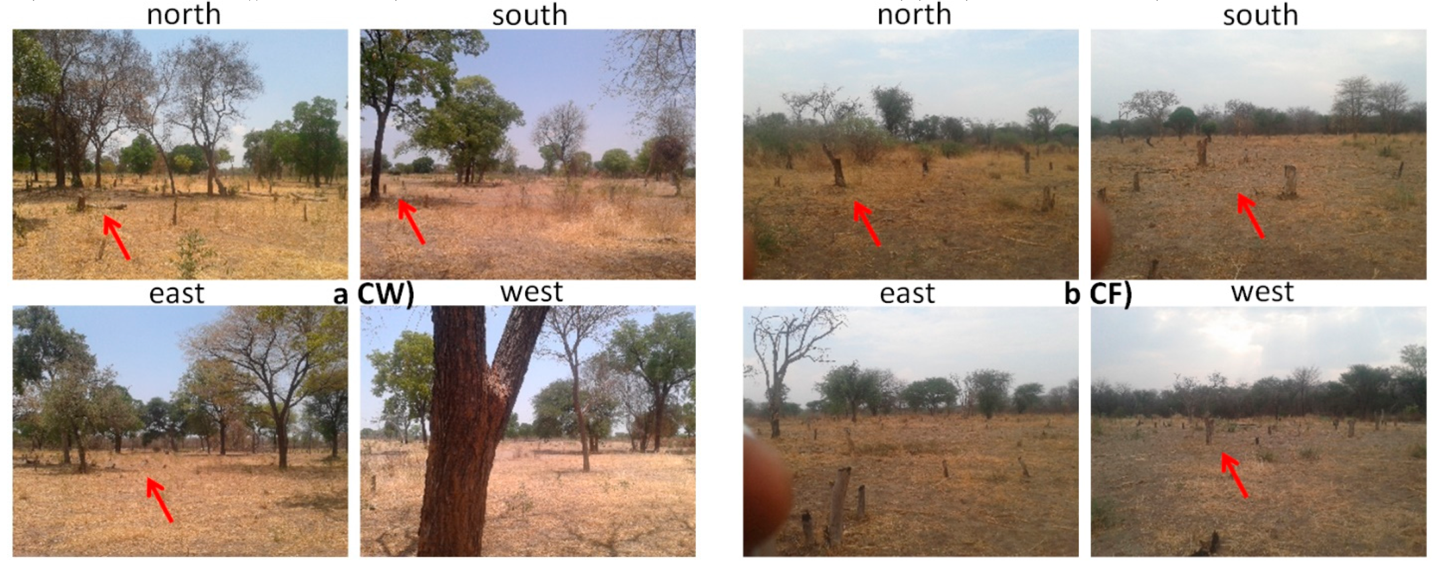
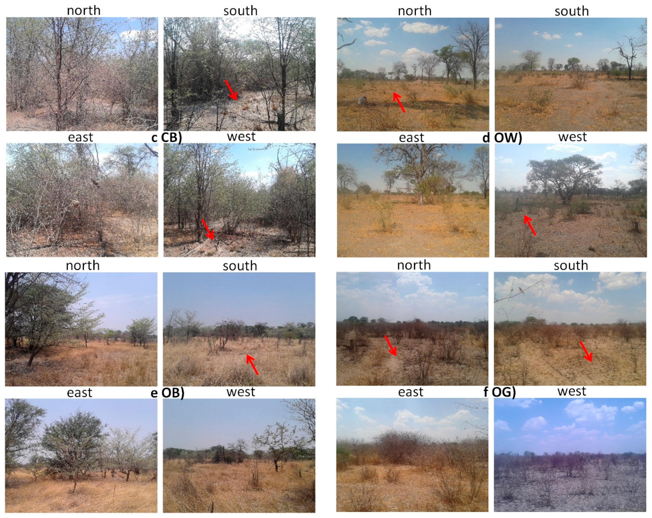
Each time series of a pixel identified by the sampling design was interpreted using TimeSync [54] and inspected with respect to whether the time series was impacted by degradation or remained unchanged for any moment in time from 2006 to 2016. During a field trip in October 2016, a total of 131 reference points located in the center of the study site were visited. Open data kit forms on smart phones were used to capture ground truth data. Date, GPS position and photos in the cardinal directions were used to report timing, location and condition of the visited plots [25]. Alongside local experts from the World Wide Fund for Nature (WWF) and the Peace Parks Foundation (PPF), the timing and observed driver of change was captured and recorded to create unambiguous plot descriptions. Questionnaires were developed to address changes within Landsat pixels of 30 m, and the interpreter in the field was asked to address environment properties within a 15 m radius. Agricultural expansion, anthropogenically caused fires and infrastructure development were found to be the most dominant land conversion processes in the area. Examples of collected ground truth of recent degradation activities for each land cover class captured during the field campaign in 2016 are shown in Figure 3. The figure shows red arrows marking visible degradation. During the field trip, it was concluded that different intensity levels of anthropogenic degradation were prominent in the visited areas, which were also characterized by differences in BFM magnitude. The most intense degradation was found in close proximity (0–160 m) to human dwellings, where the predominant land use was characterized by cultivation. Here, vegetation degradation was characterized by highly degraded landscapes through firewood collection, selective logging and burning.

2.3.3. Analysis

Comparing reference data with the produced map yields the accuracy of the map [41]. Overall accuracy, producer’s accuracy, omission error (1—producer’s accuracy) expressing the underestimation of a class, user’s accuracy, and commission error (1—user’s accuracy) expressing overestimation of a class, were calculated and reported [41,56]. According to the best practices provided by [19], accuracy estimates were corrected for true marginal map proportions [40] correcting for map class proportions as matched by the reference data based on the reference samples. Hence, confidence intervals for overall, producer’s and user’s accuracy were calculated, as well.

2.4. Land Cover-Specific Degradation Detection

Random forest [24,37] and probabilistic threshold-based [26] models were used to post-process the BFM results. Negative magnitudes are likely linked to loss of vegetation [26], while positive magnitudes can suggest an onset of vegetation growth or recovery from previous degradations [33]. Because this study focused on the measurement of degradation (removal of vegetation), any pixel characterized by a positive magnitude was discarded from further analysis. Detected BFM breakpoints with a negative magnitude are prone to errors of commission rather than omission [23]. BFMs tendency to overestimate change was reported and addressed earlier [24,26]. Each land cover type per Landsat tile was calibrated separately for degradation detection. Section 2.4.1, Section 2.4.2 and Section 2.4.3 describe three generic approaches. The three approaches were employed to understand method suitability, to identify common trends shared among them and ultimately resolve the BFM service to depict land cover specific degradation. Section 2.4.1 describes an approach to determine degradation per land cover type by the NDMI change magnitude based on probabilities, a modification of earlier work [26]. Section 2.4.2 uses a combination of SAVI and NDMI as the feature space for a random forest classification to determine degradation [24]. Section 2.4.3 combines advantages of both methods.

2.4.1. Degradation Estimation by Magnitude Threshold

The BFM magnitude provides the deviations of observed and modelled values within the monitoring period. A model was created using reference pixels depicting the ability of the NDMI magnitude to serve as method to distinguish degraded from stable land cover. For all reference points for a specific tile and land cover, the NDMI magnitude was used as a predictor variable within a binary logistic generalized linear model (GLM) for either degradation or stable land cover. Based on this, the probability of mapping degradation by magnitude was calculated for each land cover for each tile using a logistic fit for the probability $\pi$. We used a similar approach previously to determine the relationship between observation frequency and deforestation detection ability [24]. The model was constructed using ordinary least squares fitting, where ${\beta }_0$ and ${\beta }_1$ were the regression variables and $X_1$ the magnitude value. The GLM formula was:

$$ln\left(\frac{\pi }{1-\pi }\right)={\beta }_0+{\beta }_1{X}_1$$

(5)

The formula for the calculation of the probabilities was:

$$\pi =\frac{e^{{\beta }_0+{\beta }_1{X}_1}}{1+e^{{\beta }_0+{\beta }_1{X}_1}}$$

(6)

The Akaike Information Criterion (AIC) was used to determine the goodness of fit [57]. Finally, a magnitude threshold was selected for each land cover, where user’s and producer’s accuracy of change balanced out or in other words where the area bias of change was minimal. Any pixels associated with magnitudes larger than the identified magnitude threshold were treated as stable land, while smaller (more negative) magnitudes were identified as change.

2.4.2. Degradation Estimation by Random Forest Classification

Previous work identified the fusion of SAVI and NDMI magnitude features by random forest as suitable method to distinguish deforestation from stable land cover for a study site similar to KAZA [24]. We used the same combination of VIs but altered the configuration of random forest. Random forest is a supervised non-parametric classification method making use of a defined set of decision trees, a so-called forest. Each tree consists of branches (nodes) where weights of input layers are randomly varied to create a model suitable for the classification of the given feature space towards the trained classes. When executed, a reference data set is used to estimate the performance of the decision tree and potentially reiterate to find better node weights of input parameters (bootstrapping). Our random forest varied from one to 100 trees of two nodes splitting the available reference data into a 50% training fraction and a 50% validation fraction. First, the number of trees necessary to allow random forest to perform enough iterations for model creation was tested for each land cover. Secondly, the identified forest size was reiterated 100 times in a Monte Carlo approach to describe the variation in resulting accuracies by its intrinsic randomness.

2.4.3. Degradation Estimation by Combination of Magnitude Threshold and Random Forest Classification

Both methods described in Section 2.4.1 and Section 2.4.2 were combined to use their joint strength. Low-magnitude values (note that low-magnitude values are high negative values) tend to be likely linked to deforestation or degradation [26]. Any threshold set that removes high-magnitude values can result in an omission of potential changes that were high in terms of magnitude, and thus subtle events. Setting the threshold too low might result in omission of many valid changes and could result in a low producer’s accuracy of change. The opposite is true for the user’s accuracy of change and comparatively high magnitude thresholds. The advantage of random forest is the non-parametric robustness, but it lacks parametric accommodation of real-world change intensities. We chose a magnitude threshold in such a way that a producer’s accuracy of change would not drop below 80% and applied a further classification by random forest for the remaining magnitudes. Hence, a two-stage change filter was applied, where we first removed obvious or highly unlikely changes by a soft magnitude threshold and then classified the remaining portion of change to reduce the potential error of commission.

3. Results

Selected examples of the time series trajectories and BFM models for the field validation are shown in Figure 4. The time series in our study were characterized by an abundance of observations from 2013 onwards, and a low observation frequency between 1985 and 1990. Amplitude ranges for the NDMI of different land covers varied. In contrast to the other time series, CF showed the most stable time series with the least outliers and signal drops for a degradation event were clearly distinct from previous observations (history period). CW was less stable, yet degradation was distinctively identifiable in this example (Figure 4a). Both aforementioned land cover time series showed the highest NDMI values and largest amplitudes. The NDMI values for CB and OG were subtler. Values and amplitudes were low, and degradation events were not as distinct from undisturbed observations as for CW and CF. CB and OW trajectories were similar, and were characterized by medium values, amplitudes and fluctuations.

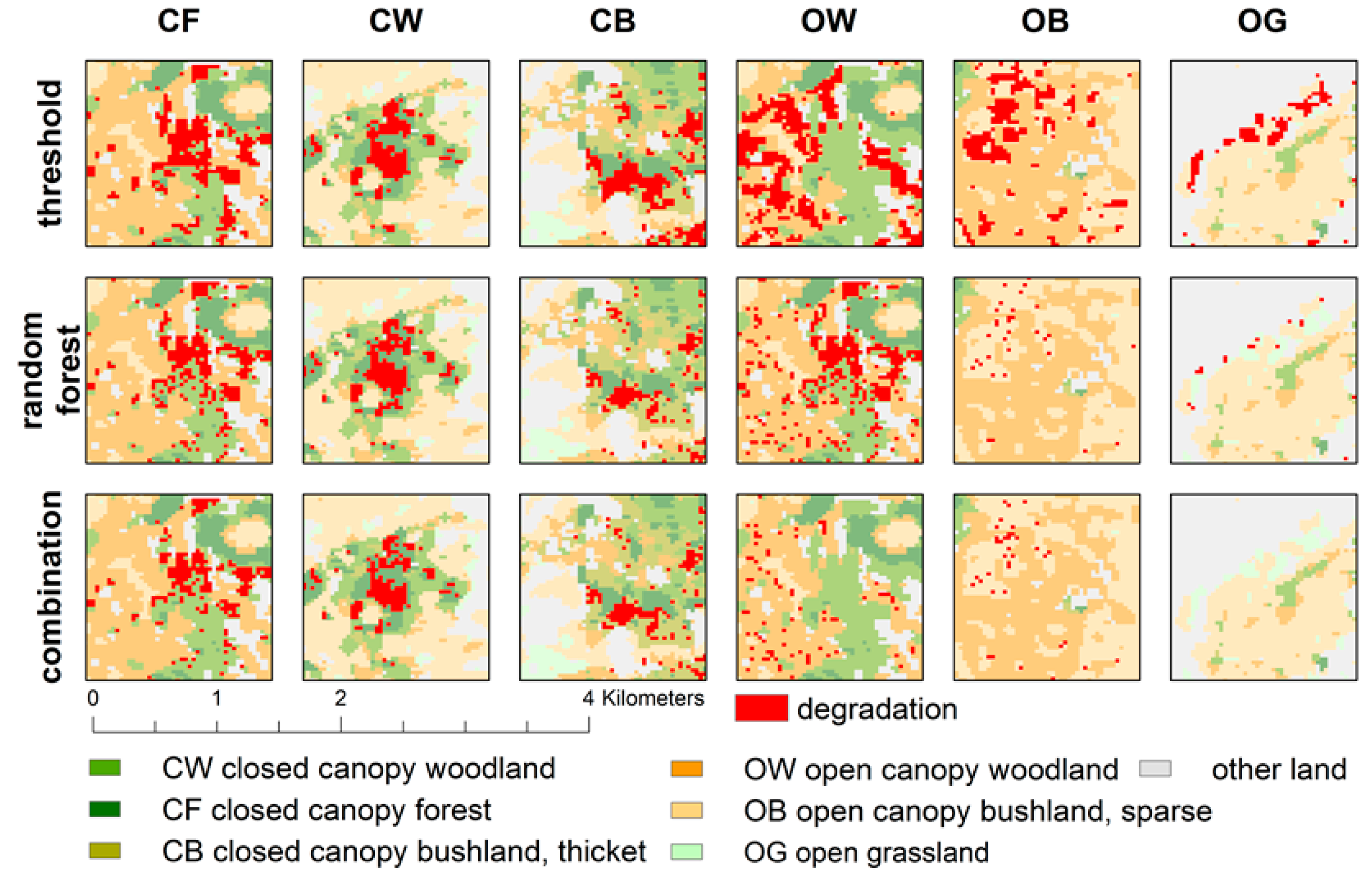
Figure 5 shows the spatial pattern of measured degradation for the selected examples. Among the methods, threshold-based degradation patterns appeared as conterminous patches, while those for random forest alone were more scattered, indicating fewer areas impacted by degradation. The random forest and threshold-based approaches combined showed the smallest amount of area impacted by degradation. The effect on the resulting detected changes was especially profound for open land cover, while changes of detected degradation across methods varied less for closed cover canopies.

3.1. Magnitude Threshold-Based Degradation Determination

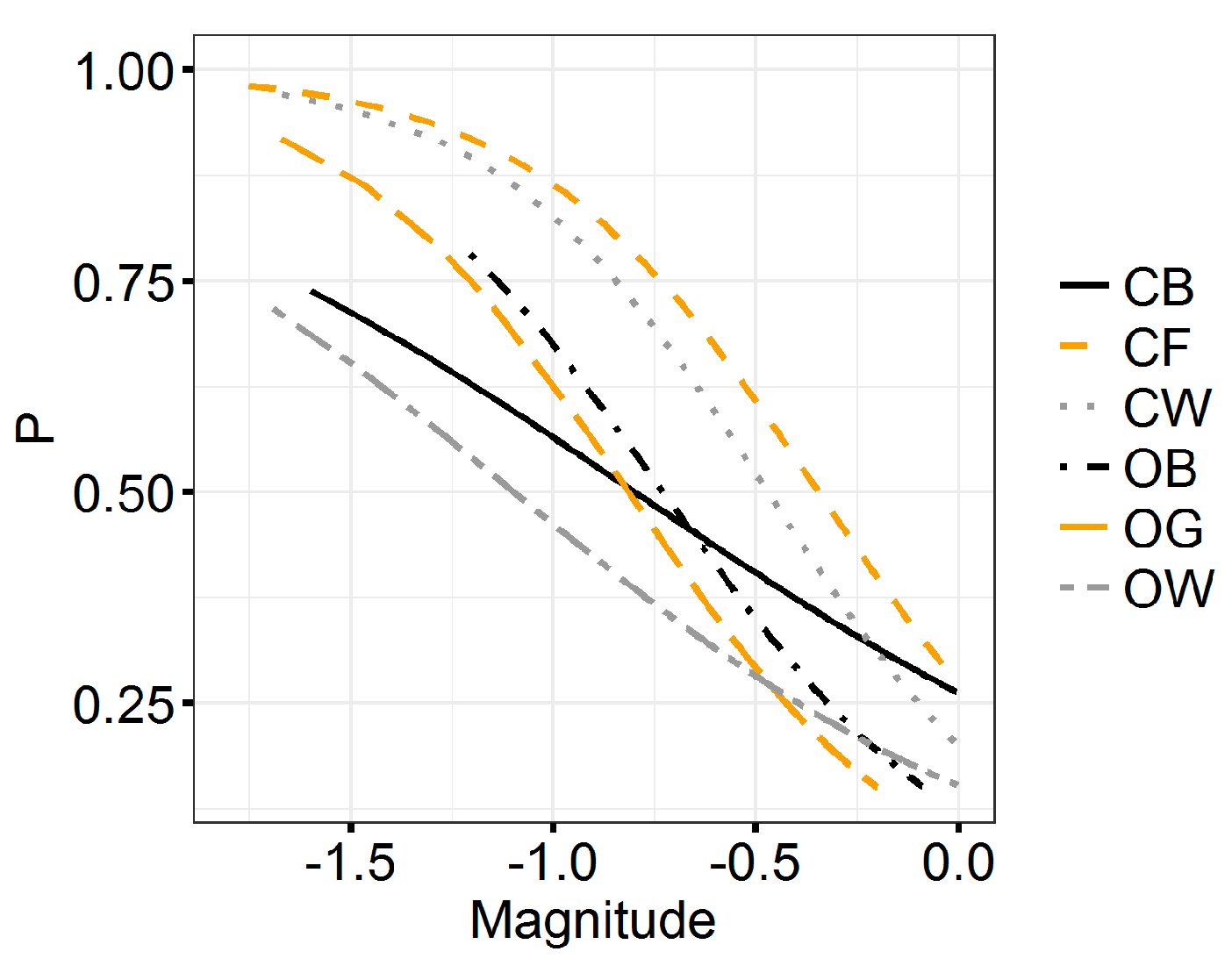
The relationship between the size of the magnitude and the probability of detecting degradation (Equation (4)) for the different land cover types is shown in Figure 6. For the sake of simplicity, within this paragraph, the term land cover refers to land cover-specific degradation. The probability of detecting degradation increased with decreasing magnitude for all classes. Differences among the relationships exist regarding the probability maxima, the shape and the position of the trajectory. These three function categories are each represented by two land cover classes. First, CW and CF were “s”-shaped functions, reaching a plateau at probabilities of 0.8–1.0. For these classes, larger magnitude values were linearly related to the probability. Furthermore, only magnitudes of these two land cover classes could identify a degradation event with high probability by using only magnitude values (where magnitude < −1.5, then p ≈ 1.0). CW and CF also showed a rapid increase in probability at rather low magnitudes (0.0–1.0). Secondly, OW and OG showed almost linear relationships between probability and magnitude. The slope of the relationship increased for class OW for magnitudes lower than −0.75, while it remained constant for OG. The maximum negative magnitude reached by OG was −1.84, and for OW it was −1.79, still suggesting that these magnitudes were not necessarily related to actual degradation events (p < 0.75). Thirdly, the functions for OB and CB were located in the middle of Figure 6. The shape of the functions was a less defined “s” shape than for the categories CW and CF, although a plateau in probability was also not reached. The slope of the two functions was located from a magnitude of −0.4 up to −1.1, similar to CF. The minimum magnitude of CB was −1.81 at a probability of 0.92, and for OB, the minimum magnitude was −1.24 at a probability of 0.79.

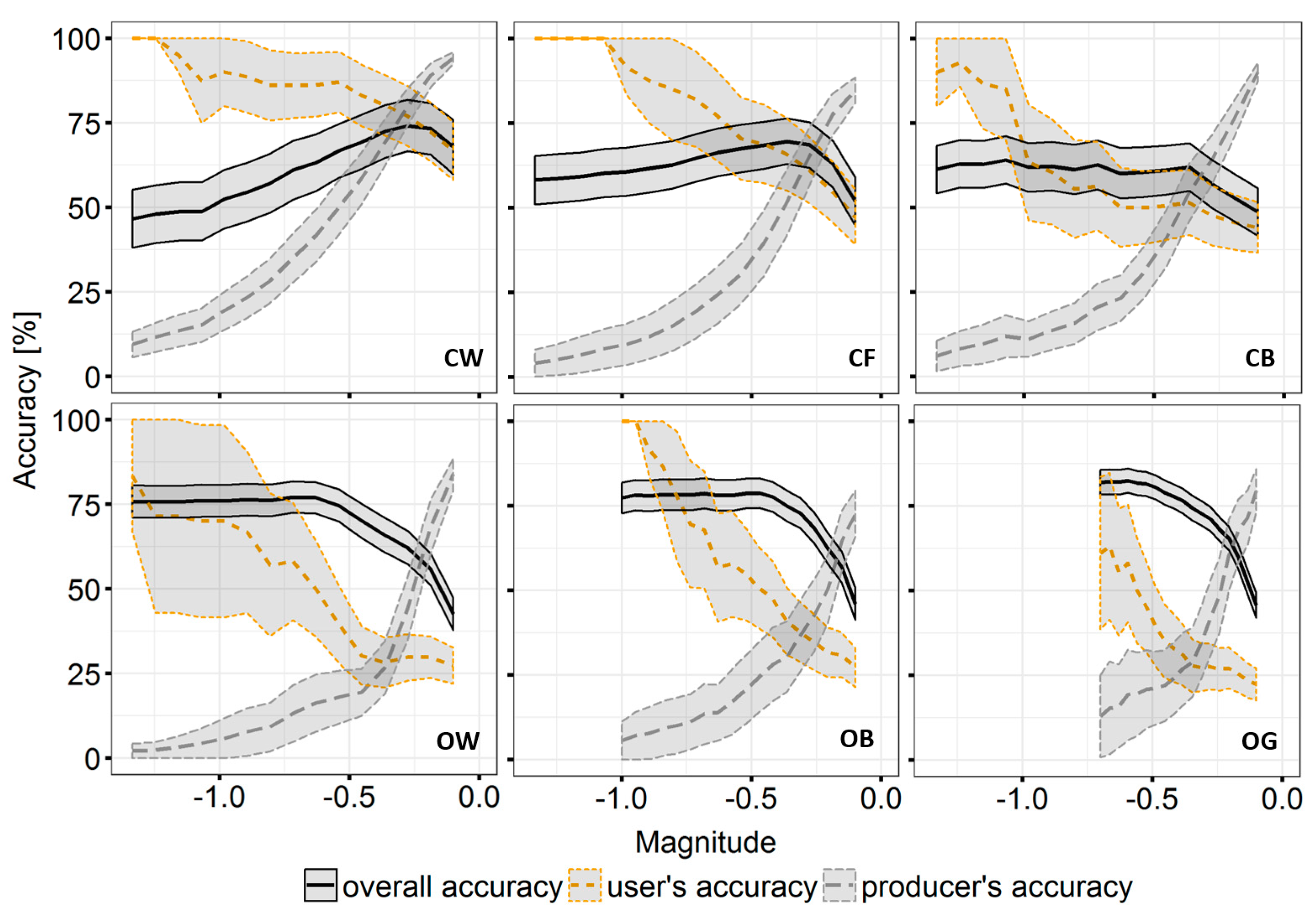
Figure 7 displays overall accuracy, user’s and producer’s accuracy, and confidence intervals for a range of magnitude thresholds for a degradation event per land cover class. The trends in accuracy in Figure 7 were similar for all classes. When the magnitude threshold was lowered, the producer’s accuracy decreased, and the user’s accuracy increased. The upper line of graphs is characterized by closed canopies (land cover CW, CF and CB) and the overall accuracy peaks at the intersection of user’s and producer’s accuracy, while for the bottom graphs, characterized by open canopies (OW, OB and OG), overall accuracy gradually increased and became saturated when the magnitude threshold was lowered. Three further phenomena were observed when the magnitude threshold was lowered. First, the confidence interval for user’s accuracy and producer’s accuracy generally increased, and diminished shortly before reaching 100% (0%, respectively, for producer’s accuracy), except for OG. For this effect, open canopies were more severely impacted than closed canopies. Lowest accuracy confidences were generally found in the mid-range of magnitude values (−0.5 to −0.9). Secondly, changes in open canopies accuracy and confidence changes occurred mostly at larger magnitudes than for closed canopies, where variations of accuracy and confidences were evident throughout the full range of negative magnitudes. As a result, the slopes of the user’s and producer’s accuracy functions were relatively flatter for closed canopies and steeper for open canopies. Closed canopies usually occupied a larger range of magnitudes, while for open canopies, major variations occurred for a short magnitude range.

3.2. Random Forest-Based Degradation Determination

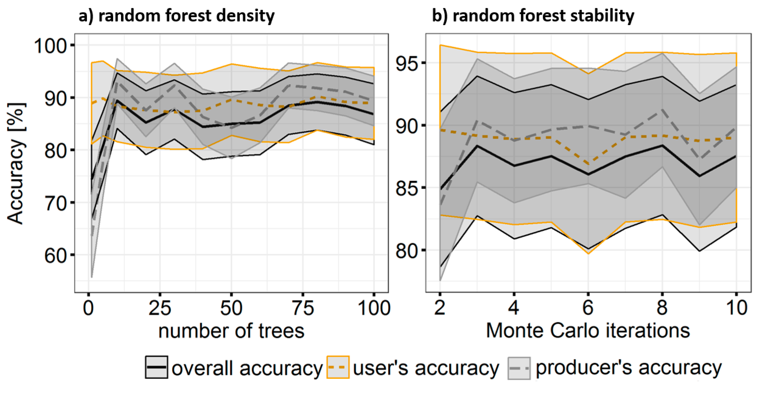
Figure 8a shows the relation between random forest tree size and its accuracy at classifying degradation events using magnitudes based on the reference data and a 50/50 training validation bootstrapping. Random forest sizes from 1–15 trees showed low producer’s accuracy for change and low overall accuracy. From 25 to 75 trees, accuracies stabilized, and no major changes in accuracy were observed. As a result, a random forest tree size of 80 was selected for all random forest classifications using the NDMI-SAVI magnitude feature spaces. Figure 8b shows the stability of the performance of the random forest classification. A Monte Carlo experiment was performed 100 times, where training and validation samples were randomly changed. A random forest model with 80 trees showed that the user’s accuracy can vary up to 3%, the producer’s accuracy up to 9%, and the overall accuracy up to 8%. The confidence interval remained fairly stable with only minor variations. The relationship between tree size and accuracies was similar for other land covers, but absolute accuracies varied. Results are summarized in Figure 9.

3.3. Combination of Magnitude Threshold and Random Forest Classification

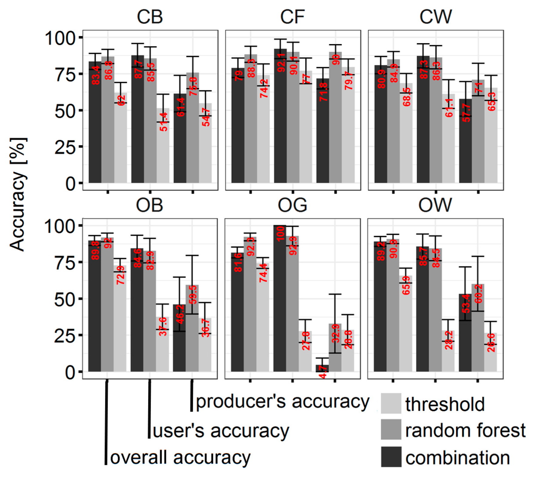
Accuracy trends were similar for the detection of land cover-specific degradation using all three methods (Figure 9). The highest combination (area bias) of producer’s and user’s accuracy was found for CF (92.1% and 90.1%, respectively). Degradation of open land cover was detected with lower accuracy than degradation of closed canopies, with open land cover classes, especially, characterized by large area estimation uncertainties (high difference between user’s and producer’s accuracy). Estimates of user’s accuracy were usually higher than those of the producer’s accuracy. For CF the user’s and producer’s accuracy were more similar in relation to the accuracies of other classes, meaning that degradation detection within this class had the lowest area bias and thus allowed for most accurate area estimations. Confidence intervals for the producer’s and user’s accuracy were different, with a confidence for user’s accuracy at about 7% and a confidence for producer’s accuracy at about 15%. Non-parametric random forest classification always outperformed probability-based threshold classification. User’s accuracy improved when random forest and the threshold classification methods were combined, while the producer’s accuracy decreased. Although random forest outperformed the threshold approach, random forest uncertainties were higher than those generated by the threshold method, especially for the producer’s accuracies of OW, OB and OG.

4. Discussion

In this study, the performance at detecting degradation of natural land cover using BFAST Monitor and Landsat NDMI and SAVI time series was assessed for different land cover classes. Within this section, the research objectives as previously stated are addressed and discussed successively. More general discussion points are provided at the end of the section.

4.1. How Does Degradation Detection Performance Differ for Six Different Land Cover Classes in KAZA Using BFM?

The performance at detecting degradation for each land cover class was most successful in the order CW, CF, CB, OW, OB and OG. The sensitivity of BFM to different land cover types, in conjunction with Enhanced Vegetation Index (EVI), was observed in a semi-arid landscape [36] and confirmed by this analysis; although we use NDMI, EVI and NDMI share similarities such as the near-infrared wavelength. For all three methods tested, the degradation for closed canopy land cover was more accurately detected than degradation within open canopy land cover types. Other studies confirm that closed canopy degradation was less prone to error than open canopy [9]. The suitability of BFM for detecting forest degradation using threshold or random forest methods has been assessed in earlier studies [24,26]. The NDMI is specifically sensitive to vegetation and its water content, which is more abundant when more vegetation is present. Since SAVI is an index that removes the effect of increasing soil exposure, it was used in combination with NDMI. The combination (using random forest) was up to 3.7 times (open woodland user’s accuracy of 100% for the combination method and 28% for the threshold-based method) more successful than using NDMI alone (threshold-based). In closed canopies and forested areas, the differences in accuracies between threshold-based, random forest and combination methods were less distinct. Confidence intervals were generally larger for user’s accuracy than for producer’s accuracy. This effect is related to the sampling design which promotes producer’s accuracy, as only areas which were identified as having potential change by BFM were sampled. A reliable independent reference data set does not yet exist for this region. Because change areas were significantly smaller than stable areas (no change detected), any mapping errors within the change class increased the uncertainty of the true marginal map proportion, resulting in a low confidence for change errors of omission while the confidence interval for errors of omission for stable land cover remained narrow. The overall accuracies shown in Figure 9 also account for stable land and are characterized by small confidence intervals, as they accommodate the confidence of both stable and change classes. With the current setup, the use of an additional independent reference data set providing knowledge of recent degradation sites can expose additional errors of omission and render existing errors of commission as correctly classified change. A similar study in Ethiopia facilitated a community-based monitoring (CBM) approach, where locals collected reference data and fed their observations into a monitoring system [38]. A similar approach might have produced a more robust reference data for the degradation monitoring system outlined in this article.

4.2. How Does Threshold Based and Random Forest-Based BFM Post-Processing for Degradation Detection Compare?

Parametric probability-based threshold selection using GLM and AIC as proposed by [26] provided comprehensible and reproducible results. In contrast, results for the non-parametric random forest classification varied due to the randomness of the method. The performance depends on tree iteration and bootstrapping, where use of reference data is a prerequisite [24]. Random forest bootstrapping tends to blur proper distinction of training and reference data, as observations are randomly swapped and shuffled to achieve the best mapping result. The use of random forest in conjunction with field data has been deemed an appropriate and successful tool in similar environments [38,43], although its error margins have not been determined. Although the magnitude threshold-based approach can be more intuitive, it fails to depict the ecosystem complexity and its related degradation processes. Typically, the random forest machine learning approach will fail to produce the same result as demonstrated in Figure 8b.

4.3. How Are Method Variations Impacting Degradation Detection Accuracy and How to Combine Threshold-Based and Random Forest-Based BFM Post-Processing Methods Effectively?

Across observed land cover types, the impact of a decrease in magnitude as threshold on the confidence interval varied, because degradation reference points were gradually allocated to stable land with a decrease in magnitude (more negative). This reduced confidence in the producer’s accuracy for degradation. As the confidence interval of the producer’s accuracy for degradation increased, the user’s accuracy simultaneously increased, along with the confidence interval. Figure 10 reveals that the confidence intervals and accuracy for stable land cover were tending in the opposite direction from the degraded areas, but changes and expansion of the confidence interval were lower, as their area is larger, and thus an increase in error introduced by true marginal map proportions is less severe. Changing the magnitude threshold affected the accuracy but, more importantly, also the accuracy confidence, especially for open canopies, where confusion (error rate) was higher. Random forest, on the other hand, was solely impacted by the number of trees and its internal randomness. As a result, the accuracy varied, but confidence remained stable if iterations were kept stable (Figure 8). When threshold-based degradation detection alone was used, optimal results were achieved at the intersection of user’s and producer’s accuracy for change [26]. When combined with random forest particularly the commission of change was suppressed, and the magnitude threshold should be set as conservatively and subtle as possible to avoid any omission of degradation. Pixels characterized by very small magnitudes and by high probabilities of degradation (p > 0.8) can be considered an accurate degradation detection, while remaining pixels can be subject to more selective random forest classification. The combination of both methods secured pixels that were almost certain, having changed using a threshold-based method, whereas more complex changes were addressed by random forest.

5. Conclusions

Landsat NDMI time series analysis using BFM detected degradation of heavily vegetated areas within large savannah landscapes, especially when tree cover was high (CW and CF). Distinct signal drops of BFM change magnitude were used in non-parametric and parametric approaches to detect degradations. As vegetation cover decreased, the performance of degradation detection dropped. When combining NDMI and SAVI at the feature level, detection performance increased, especially for sparse vegetation cover. Hence, different land cover degradations require specific VIs for accurate monitoring programs. In comparison, non-parametric random forest was found to be more accurate at detecting change than a threshold-based approach. Especially confidence intervals were affected by the threshold-based approached, when the magnitude threshold varied. Large-area monitoring programs covering different ecosystems and land cover types therefore require specific VI time series and an individual BFM model calibration. Variations in BFM harmonic order, different models to address model history or BFM sequential approaches (for instance, year-wise monitoring) also require specific VIs and land cover-specific adjustments. Alternatively, spectral endmember-based approaches have shown promising results for forested landscapes [24,58], and therefore, specific land cover endmembers can be of use for different sets of land cover types. Implementing a CBM campaign driven by local experts, as done in [38], within KAZA could produce a stronger reference data set, and therefore allow more detailed conclusions of the proposed method for the different vegetation types. Increasing observation frequency could also increase the probability of detecting degradation events [24,27]. Hence, incorporating other data sources such as Sentinel 1 and 2 is desirable, as observation frequency could be increased at no-cost [28]. Dense time series within the monitoring period will result in fewer errors of omission [21]. Data fusion with Sentinel 1 and other synthetic aperture radar (SAR) devices, as suggested previously [27], could improve both historic period observation frequency, and therefore BFAST Monitor models and monitoring performance. Furthermore, SAVI and NDMI degradation detection performances were low for open canopy forest Vis, which are more sensitive to these forest types, and differences in canopy cover can yield higher performances. For instance, the normalized difference fraction index (NDFI) was identified to be sensitive to different degrees of canopy cover [58]. In summary, increasing observation frequency by incorporating Sentinel data and the application of canopy cover-sensitive VIs yields promising prospects for further improving degradation detection accuracy for open canopy forests.

References

1. Naidoo, R.; Preez, P.D.; Stuart-Hill, G.; Beytell, P.; Taylor, R. Long-range migrations and dispersals of African buffalo (Syncerus caffer) in the Kavango–Zambezi Transfrontier Conservation area. Afr. J. Ecol. 2014, 52, 581–584. [Google Scholar] [CrossRef]
2. Naidoo, R.; Fisher, B.; Manica, A.; Balmford, A. Estimating economic losses to tourism in Africa from the illegal killing of elephants. Nat. Commun. 2016, 7, 13379. [Google Scholar] [CrossRef] [PubMed] [Green Version]
3. Metcalfe, S.; Kepe, T. ‘Your Elephant on Our Land’ The Struggle to Manage Wildlife Mobility on Zambian Communal Land in the Kavango-Zambezi Transfrontier Conservation Area. J. Environ. Dev. 2008, 17, 99–117. [Google Scholar] [CrossRef]
4. Scholz, I.; Schmidt, L. Reducing Emissions from Deforestation and Forest Degradation in Developing Countries: Meeting the Main Challenges Ahead; Deutsches Institut für Entwicklungspolitik Bonn: Bonn, Germany, 2008. [Google Scholar]
5. Herold, M.; Skutsch, M. Monitoring, reporting and verification for national REDD + programmes: Two proposals. Environ. Res. Lett. 2011, 6, 14002. [Google Scholar] [CrossRef]
6. TÜV SÜD. Reducing Emissions from Deforestation and Carbon Enhancement from in Xe Pian National Protected Area, Lao PDR; Environmental Technology, Carbon Management Service Solitaire, I.T.I. Road, Aundh, Pune-411007, INDIA: Noida, India, 2018. [Google Scholar]
7. Nellemann, C. Green Carbon, Black Trade: Illegal Logging, Tax Fraud and Laundering in the World’s Tropical Forests; United Nations Environment Programme, GRID-Arendal: Arendal, Norway, 2012. [Google Scholar]
8. Petit, C.; Scudder, T.; Lambin, E. Quantifying processes of land-cover change by remote sensing: Resettlement and rapid land-cover changes in south-eastern Zambia. Int. J. Remote Sens. 2001, 22, 3435–3456. [Google Scholar] [CrossRef]
9. Kamwi, J.M.; Kaetsch, C.; Graz, F.P.; Chirwa, P.; Manda, S. Trends in land use and land cover change in the protected and communal areas of the Zambezi Region, Namibia. Environ. Monit. Assess. 2017, 189, 242. [Google Scholar] [CrossRef] [PubMed]
10. Wingate, V.R.; Phinn, S.R.; Kuhn, N.; Bloemertz, L.; Dhanjal-Adams, K.L. Mapping decadal land cover changes in the woodlands of north eastern Namibia from 1975 to 2014 using the Landsat satellite archived data. Remote Sens. 2016, 8, 681. [Google Scholar] [CrossRef]
11. Mason, S.J. El Niño, climate change, and Southern African climate. Environmetrics 2001, 12, 327–345. [Google Scholar] [CrossRef]
12. Roy, D.P.; Boschetti, L.; Justice, C.O.; Ju, J. The collection 5 MODIS burned area product—Global evaluation by comparison with the MODIS active fire product. Remote Sens. Environ. 2008, 112, 3690–3707. [Google Scholar] [CrossRef]
13. Pekel, J.-F.; Cottam, A.; Gorelick, N.; Belward, A.S. High-resolution mapping of global surface water and its long-term changes. Nature 2016, 540, 418–422. [Google Scholar] [CrossRef] [PubMed]
14. Avitabile, V.; Herold, M.; Heuvelink, G.B.; Lewis, S.L.; Phillips, O.L.; Asner, G.P.; Armston, J.; Ashton, P.S.; Banin, L.; Bayol, N.; et al. An integrated pan-tropical biomass map using multiple reference datasets. Glob. Chang. Biol. 2016, 22, 1406–1420. [Google Scholar] [CrossRef] [PubMed] [Green Version]
15. Pricope, N.G.; Gaughan, A.E.; All, J.D.; Binford, M.W.; Rutina, L.P. Spatio-Temporal Analysis of Vegetation Dynamics in Relation to Shifting Inundation and Fire Regimes: Disentangling Environmental Variability from Land Management Decisions in a Southern African Transboundary Watershed. Land 2015, 4, 627–655. [Google Scholar] [CrossRef] [Green Version]
16. Lambin, E.F.; Ehrlich, D. Land-cover changes in sub-Saharan Africa (1982–1991): Application of a change index based on remotely sensed surface temperature and vegetation indices at a continental scale. Remote Sens. Environ. 1997, 61, 181–200. [Google Scholar] [CrossRef]
17. Brink, A.B.; Eva, H.D. Monitoring 25 years of land cover change dynamics in Africa: A sample based remote sensing approach. Appl. Geogr. 2009, 29, 501–512. [Google Scholar] [CrossRef] [Green Version]
18. Mosugelo, D.K.; Moe, S.R.; Ringrose, S.; Nellemann, C. Vegetation changes during a 36-year period in northern Chobe National Park, Botswana. Afr. J. Ecol. 2002, 40, 232–240. [Google Scholar] [CrossRef]
19. Olofsson, P.; Foody, G.M.; Herold, M.; Stehman, S.V.; Woodcock, C.E.; Wulder, M.A. Good practices for estimating area and assessing accuracy of land change. Remote Sens. Environ. 2014, 148, 42–57. [Google Scholar] [CrossRef] [Green Version]
20. Woodcock, C.E.; Allen, R.G.; Anderson, M.; Belward, A. Free Access to Landsat Imagery. Science 2008, 320, 5879. [Google Scholar] [CrossRef] [PubMed]
21. Hansen, M.C.; Potapov, P.V.; Moore, R.; Hancher, M.; Turubanova, S.A.; Tyukavina, A.; Thau, D.; Stehman, S.V.; Goetz, S.J.; Loveland, T.R.; et al. High-Resolution Global Maps of 21st-Century Forest Cover Change. Science 2013, 342, 850–853. [Google Scholar] [CrossRef] [PubMed]
22. Verbesselt, J.; Hyndman, R.; Zeileis, A.; Culvenor, D. Phenological change detection while accounting for abrupt and gradual trends in satellite image time series. Remote Sens. Environ. 2010, 114, 2970–2980. [Google Scholar] [CrossRef] [Green Version]
23. Schultz, M.; Verbesselt, J.; Avitabile, V.; Souza, C.; Herold, M. Error Sources in Deforestation Detection Using BFAST Monitor on Landsat Time Series Across Three Tropical Sites. IEEE J. Sel. Top. Appl. Earth Obs. Remote Sens. 2015, 9, 3667–3679. [Google Scholar] [CrossRef]
24. Schultz, M.; Clevers, J.; Carter, S.; Verbesselt, J.; Avitabile, V.; Hien, V.Q. Performance of vegetation indices from Landsat time series in deforestation monitoring. Int. J. Appl. Earth Obs. Geoinf. 2016, 52, 318–327. [Google Scholar] [CrossRef]
25. Pratihast, A.K.; DeVries, B.; Avitabile, V.; de Bruin, S.; Kooistra, L.; Tekle, M.; Herold, M. Combining satellite data and community-based observations for forest monitoring. Forests 2014, 5, 2464–2489. [Google Scholar] [CrossRef]
26. DeVries, B.; Verbesselt, J.; Kooistra, L.; Herold, M. Robust monitoring of small-scale forest disturbances in a tropical montane forest using Landsat time series. Remote Sens. Environ. 2015, 161, 107–121. [Google Scholar] [CrossRef]
27. Reiche, J.; Verbesselt, J.; Hoekman, D.H.; Herold, M. Fusing Landsat and SAR time series to detect deforestation in the tropics. Remote Sens. Environ. 2015, 156, 276–293. [Google Scholar] [CrossRef]
28. Reiche, J.; Hamunyela, E.; Verbesselt, J.; Hoekman, D.; Herold, M. Improving near-real time deforestation monitoring in tropical dry forests by combining dense Sentinel-1 time series with Landsat and ALOS-2 PALSAR-2. Remote Sens. Environ. 2018, 204, 147–161. [Google Scholar] [CrossRef]
29. Verbesselt, J.; Zeileis, A.; Herold, M. Near real-time disturbance detection using satellite image time series. Remote Sens. Environ. 2012, 123, 98–108. [Google Scholar] [CrossRef]
30. Dutrieux, L.P.; Verbesselt, J.; Kooistra, L.; Herold, M. Monitoring forest cover loss using multiple data streams, a case study of a tropical dry forest in Bolivia. ISPRS J. Photogramm. Remote Sens. 2015, 107, 112–125. [Google Scholar] [CrossRef]
31. Jakovac, C.C.; Dutrieux, L.P.; Siti, L.; Peña-Claros, M.; Bongers, F. Spatial and temporal dynamics of shifting cultivation in the middle-Amazonas river: Expansion and intensification. PLoS ONE 2017, 12, e0181092. [Google Scholar] [CrossRef] [PubMed]
32. Dutrieux, L.P.; Jakovac, C.C.; Latifah, S.H.; Kooistra, L. Reconstructing land use history from Landsat time-series: Case study of a swidden agriculture system in Brazil. Int. J. Appl. Earth Obs. Geoinf. 2016, 47, 112–124. [Google Scholar] [CrossRef]
33. DeVries, B.; Decuyper, M.; Verbesselt, J.; Zeileis, A.; Herold, M.; Joseph, S. Tracking disturbance-regrowth dynamics in tropical forests using structural change detection and Landsat time series. Remote Sens. Environ. 2015, 169, 320–334. [Google Scholar] [CrossRef]
34. Murillo-Sandoval, P.J.; van den Hoek, J.; Hilker, T. Leveraging Multi-Sensor Time Series Datasets to Map Short-and Long-Term Tropical Forest Disturbances in the Colombian Andes. Remote Sens. 2017, 9, 179. [Google Scholar] [CrossRef]
35. Maynard, J.J.; Karl, J.W.; Browning, D.M. Effect of spatial image support in detecting long-term vegetation change from satellite time-series. Landsc. Ecol. 2016, 31, 2045–2062. [Google Scholar] [CrossRef]
36. Watts, L.M.; Laffan, S.W. Effectiveness of the BFAST algorithm for detecting vegetation response patterns in a semi-arid region. Remote Sens. Environ. 2014, 154, 234–245. [Google Scholar] [CrossRef]
37. Breiman, L. Random forests. Mach. Learn. 2001, 45, 5–32. [Google Scholar] [CrossRef]
38. DeVries, B.; Pratihast, A.K.; Verbesselt, J.; Kooistra, L.; Herold, M. Characterizing forest change using community-based monitoring data and Landsat time series. PLoS ONE 2016, 11, e0147121. [Google Scholar] [CrossRef] [PubMed]
39. Urbazaev, M.; Thiel, C.; Migliavacca, M.; Reichstein, M.; Rodriguez-Veiga, P.; Schmullius, C. Improved Multi-Sensor Satellite-Based Aboveground Biomass Estimation by Selecting Temporally Stable Forest Inventory Plots Using NDVI Time Series. Forests 2016, 7, 169. [Google Scholar] [CrossRef]
40. Card, D.H. Using known map category marginal frequencies to improve estimates of thematic map accuracy. Am. Soc. Photogramm. 1982, 48, 431–439. [Google Scholar]
41. Congalton, R. A review of assessing the accuracy of classifications of remotely sensed data. Remote Sens. Environ. 1991, 37, 35–46. [Google Scholar] [CrossRef]
42. Liu, J.; Heiskanen, J.; Maeda, E.E.; Pellikka, P.K. Burned area detection based on Landsat time series in savannas of southern Burkina Faso. Int. J. Appl. Earth Obs. Geoinf. 2018, 64, 210–220. [Google Scholar] [CrossRef]
43. Pratihast, A.K.; DeVries, B.; Avitabile, V.; de Bruin, S.; Herold, M.; Bergsma, A. Design and implementation of an interactive web-based near real-time forest monitoring system. PLoS ONE 2016, 11, e0150935. [Google Scholar] [CrossRef] [PubMed]
44. Gao, B.-C. NDWI—A normalized difference water index for remote sensing of vegetation liquid water from space. Remote Sens. Environ. 1996, 58, 257–266. [Google Scholar] [CrossRef]
45. Huete, A.R. A soil-adjusted vegetation index (SAVI). Remote Sens. Environ. 1988, 25, 295–309. [Google Scholar] [CrossRef]
46. Miura, T.; Huete, A.R.; van Leeuwen, W.J.D.; Didan, K. Vegetation detection through smoke-filled AVIRIS images: An assessment using MODIS band passes. J. Geophys. Res. Atmos. 1998, 103, 32001–32011. [Google Scholar] [CrossRef] [Green Version]
47. Hayes, D.J.; Cohen, W.B.; Sader, S.A.; Irwin, D.E. Estimating proportional change in forest cover as a continuous variable from multi-year MODIS data. Remote Sens. Environ. 2008, 112, 735–749. [Google Scholar] [CrossRef] [Green Version]
48. Thompson, M. Land-Cover Classification for Peace Parks, KAZA Extension for Namibia, Botswana, Zimbabwe and Zambia—Data Users Report and Meta Data; GeoTerraImage: Pretoria, South Africa, 2014. [Google Scholar]
49. Masek, J.; Vermote, E.F.; Saleous, N.; Wolfe, R.; Hall, F.G.; Huemmrich, F.; Gao, F.; Kutler, J.; Lim, T.K. LEDAPS Landsat Calibration, Reflectance, Atmospheric Correction Preprocessing Code; NASA: Oak Ridge, TN, USA, 2012.
50. USGS. Landsat Processing Details; USGS: Sioux Falls, SD, USA, 2016.
51. Roy, D.P.; Borak, J.S.; Devadiga, S.; Wolfe, R.E.; Zheng, M.; Descloitres, J. The MODIS land product quality assessment approach. Remote Sens. Environ. 2002, 83, 62–76. [Google Scholar] [CrossRef]
52. Zhu, Z.; Woodcock, C.E. Object-based cloud and cloud shadow detection in Landsat imagery. Remote Sens. Environ. 2012, 118, 83–94. [Google Scholar] [CrossRef]
53. Foody, G.M. Sample size determination for image classification accuracy assessment and comparison. Int. J. Remote Sens. 2009, 30, 5273–5291. [Google Scholar] [CrossRef]
54. Cohen, W.B.; Yang, Z.; Kennedy, R. Detecting trends in forest disturbance and recovery using yearly Landsat time series: 2. TimeSync—Tools for calibration and validation. Remote Sens. Environ. 2010, 114, 2911–2924. [Google Scholar] [CrossRef]
55. Strahler, A.H.; Boschetti, L.; Foody, G.M.; Friedl, M.A.; Hansen, M.C.; Herold, M.; Morisette, J.T.; Stehman, S.V.; Woodcock, C.E. Global Land Cover Validation: Recommendations for Evaluation and Accuracy Assessment of Global Land Cover Maps; JRC European Commission: Brussels, Belgium, 2006. [Google Scholar]
56. Congalton, R.G.; Green, K. Assessing the Accuraccy of Remotely Sensed Data Principles and Practices; CRC Press: New York, NY, USA, 2009. [Google Scholar]
57. Akaike, H. Information Theory and an Extension of the Maximum Likelihood Principle. In The Second International Symposium on Information Theory; Akademiai Kiado: Budapest, Hungary, 1973; pp. 267–281. [Google Scholar]
58. Souza, C.M., Jr.; Roberts, D.A.; Cochrane, M.A. Combining spectral and spatial information to map canopy damage from selective logging and forest fires. Remote Sens. Environ. 2005, 98, 329–343. [Google Scholar] [CrossRef]
Figure 1. (a) Black lines are borders of countries covered by Kavango Zambezi Transfrontier Conservation Area (KAZA) (blue blob), clockwise from top left: Angola, Zambia, Zimbabwe, Botswana and Namibia; (b) land cover in 2005 for the KAZA study site, grey frames show Landsat tiles used; (c) shown in the blue subset of the KAZA green ribbon, dots are the examples of land cover sites visited during field trip where degradation occurred as displayed in Figure 3.
Remotesensing 10 01850 g001
Figure 2. Overview of the methods applied in this study.
Remotesensing 10 01850 g002
Figure 3. Examples of collected ground truth of recent degradation activities for each land cover class captured during a field campaign in October 2016; red arrows mark visible degradation for (a) closed canopy woodland (CW), where tree trunks outnumber existing trees; (b) closed canopy forest (CF), where tree trunks indicate previous forest density; (c) closed canopy bushland (CB), where footpaths and broken trees indicate firewood collection; (d) thicket open canopy woodland (OW), where tree trunks and footpaths are visible; (e) open canopy bushland (OB), where footpaths are visible; (f) sparse open grassland (OG), where traces of animal and human footprints are visible.
Remotesensing 10 01850 g003aRemotesensing 10 01850 g003b
Figure 4. Black points of NDMI values displayed as time series trajectories and its BFM model allocated within the considered land cover classes; left side of the vertical black line shows the historic period, the right side the monitoring period; vertical dotted line indicates a breakpoint as detected by BFM; blue lines depict the linear and harmonic components of the model.
Remotesensing 10 01850 g004
Figure 5. Examples of mapped land cover-specific degradation shown in red for the different methods used.
Remotesensing 10 01850 g005
Figure 6. Probabilities (P) for detecting a deforestation event in relation to the magnitude for the specific land cover classes.
Remotesensing 10 01850 g006
Figure 7. Land cover degradation-specific accuracies in relation to the magnitude threshold; grey ribbons show confidence interval.
Remotesensing 10 01850 g007
Figure 8. (a) Relationship between accuracy and the number of trees used for random forest classification for class CF (closed canopy forest); (b) variation of accuracy due to random forest randomness when using 80 trees across 100 iterations.
Remotesensing 10 01850 g008
Figure 9. Grouped bar plot of land cover specific accuracies for detecting degradation compared by method; whiskers show confidence interval.
Remotesensing 10 01850 g009
Figure 10. Relationship of accuracy and confidence interval with change magnitude for stable and degraded land cover type OW (open canopy woodland).
Remotesensing 10 01850 g010