1. Introduction
Weather monitoring and particularly nowcasting is currently based on two major data sources: rapid update weather forecast [
1,
2] and weather radars [
3,
4], providing information about current weather and short term forecasts. However, weather radars are very expensive and observations may be affected by several errors such as echo lines, topography, canopy and building shadowing effects as well as rain bands reduction [
5]. For over two decades, ground-based GNSS networks have been used for operational positioning and collecting data time series in order to better understand interference on transmitted radio waves. The dependency on tropospheric conditions revealed the remote sensing application of GNSS signals [
6,
7]. The total tropospheric delay is usually expressed in zenith direction, hence it is called zenith total delay (ZTD). Its conversion into Integrated Water Vapor (IWV) has become a routine in nowadays GNSS data processing within Network of European Meteorological Services (EUMETNET) EIG GNSS Water Vapour Programme (E-GVAP, egvap.dmi.dk) and activities of ESSEM COST Action ES1206 “Advanced Global Navigation Satellite Systems tropospheric products for monitoring severe weather events and climate (GNSS4SWEC)” (gnss4swec.knmi.nl). Assimilation of GNSS ZTD into Numerical Weather Prediction (NWP) models [
8,
9,
10] has helped to reduce forecast uncertainty. The delay in the direction to the satellite, i.e., the slant total delay (STD) contains full information of the troposphere along the propagation path. Currently, improvement of weather models based on GNSS STDs stands a challenge in variational assimilation [
11,
12].
Ray-tracing has become a common technique to provide independent values of tropospheric delays [
13,
14]. Contrary to ground-based GNSS delays that rely on clocks, orbits and associated pseudoranges [
15], ray-tracing uses NWP model variables. Thus, it serves as a forward observation operator in variational assimilation which allows converting model data into geodetic observations [
16]. With ray-tracing we are able to compute tropospheric delays for ground station in the specified elevation angle and azimuth associated with satellite position as long as the weather model is available. The precision of ray-traced delays with respect to GNSS estimates is reported to be at the 1-cm level in terms of standard deviation of ZTD [
17].
In the neutral atmosphere, the major contribution to the tropospheric delay comes from gaseous constituents that form hydrostatic and wet components of the delay. The hydrostatic delay is proportional to air pressure, whereas the wet part is related to temperature and water vapor content. As the GNSS signals sit in the L band of the microwave spectrum, they are almost insensitive to the hydrometeors. Hence, the effect of liquid and solid particles suspended in the air is usually neglected in the tropospheric delays since the impact is a few orders of magnitude smaller than other air constituents [
18].
The significance of hydrometeors becomes important during weather phenomena that produce heavy rainfalls or snow, fog and dust storms which are usually connected with the large amount of clouds. Various particles are expected to induce 3% of the delay compared to that caused by dry air and water vapor [
18]. Douša et al. [
19] reported that the difference between maximum and minimum slant delay mapped to the zenith direction due to the presence of hydrometeors is on the level of 1 cm. Number of studies attempted to characterize local atmospheric structures using GNSS products and associated variables as an indicator. De Haan et al. [
20] analyzed tropospheric delays during cold front passage and demonstrated azimuth-elevation anisotropy visible in the wet delay component. Brenot et al. [
21] simulated and observed ZTDs during extreme weather event to quantify the impact of hydrometeors, they attained maximum 30 mm delay. The Saastamoinen formulation of hydrostatic delay [
22] applied in the presence of high hydrometeor contribution is expected to overestimate the total delay. Application of ZTD and horizontal gradients in the study of Brenot et al. [
23] allowed to point out convection cells during heavy rainfall event, where wet gradients appeared to increase towards its direction. Shoji et al. [
24] used similar methodology to indicate severe weather based on estimated precipitable water vapor gradient calculated from ZTD and mapped STD. In the recent study, Masoumi et al. [
25] presented effects of improper modeling in GNSS data processing induced by horizontal gradients [
26] which may affect estimated tropospheric delays in particular weather conditions.
In this paper, we use GNSS observations and ray-tracing technique to find a potential correlation between rain, clouds and tropospheric delays. We use cases with intense rainfalls observed over Poland during the period of GNSS4SWEC Benchmark campaign [
19]. In our approach, we model ray-traced STDs using Weather Research and Forecasting (WRF) model assuming that the signal propagates in the atmosphere that is a pure gas. Thus, it theoretically depends only on pressure, temperature and water vapor pressure, but it also reflects the model accuracy. On the other hand, the GNSS observations provide slant delays with total atmospheric contribution. Hence, the influence of neglected liquid and solid particles should be visible in calculated GNSS estimates reduced by ray-traced delays. In severe atmospheric conditions, these residuals should surpass the uncertainty level of estimated tropospheric delays. Both GNSS and ray-traced delays need to be provided with superior accuracy in order to properly distinguish troposphere-induced effects from other systematic effects. In the normal equation system GNSS STDs cannot be estimated directly as the number of unknown parameters exceeds number of observations. Thus, GNSS retrievals will absorb part of the uncertainty introduced by assumptions and constraints such as mapping functions and phase ambiguity. The other data source of ray-traced retrievals is affected by uncertainty of meteorological background and assumptions for the propagation of electromagnetic field. The paper provides a detailed analysis of data uncertainties and a comprehensive error propagation for tropospheric estimates to reveal effects of atmospheric liquid and solid water absorbed in GNSS signal.
The novel approach in this study is the application of GNSS STDs to assess the potential to retrieve impact of hydrometeors on independent ray-traced retrievals. The saturation of air with liquid and solid particles is indicated based on cloud type remote sensing measurements and rain rate satellite observations. For easier interpretation of residual magnitudes, the computed differences in tropospheric delays are mapped to the zenith direction. The paper is organized as follows: in
Section 2 we present our approach to ray-trace the GNSS signal from ground station to satellite.
Section 3 shows the applied GNSS STD estimation strategy. In the next chapter, we introduce meteorological observations used in our study. In
Section 5 and
Section 6, an overview of the data quality is presented and discussed.
Section 7 presents statistics for GNSS stations involved in the analysis to demonstrate the impact of hydrometeors on GNSS tropospheric delays. The paper is closed with a conclusion.
2. Ray-Path Model
The ray-tracing technique is used to calculate tropospheric delays in WRF model. We follow similar methodology to Böhm et al. [
27] which has been operationally applied to provide forecast Vienna Mapping Functions (VMF1). Wilgan et al. [
28] showed that application of our ray-tracer to derive WRF-based mapping function results in comparable performance to VMF1-FC Böhm et al. [
29] in terms of position and can help to improve convergence time in real-time PPP. The ray-tracing algorithm is based on the geometrical optics approximation and assumes the signal to propagate within the plane of a constant azimuth. Since horizontal gradients in the troposphere are generally much lower than vertical gradients [
30], the perpendicular contribution to the ray-path is neglected which makes the trajectory two-dimensional (no out-of-plane components). The signal delay is considered to be a phase excess introduced by the atmospheric refraction
n along the ray-path trajectory. It causes the path length to differ from its geometric straight-line distance
S [
31] according to the equation
Here, we separate the signal path into finite number of linear ray-pieces along the bent ray-path. The refractive index
n or alternatively refractivity
N describes the medium properties and its impact on radio propagation. The fundamental variables necessary to express atmospheric state in terms of gaseous properties are: the air pressure
(hPa), the air temperature
T (K) and the water vapor partial pressure
(hPa) that form the equation valid for GNSS frequencies according to Davis et al. [
7]
with
being atmospheric density that can be described as a relation
where
and
are molar masses of dry and wet air respectively and
is the universal gas constant. The values
,
and
denote empirically derived refractivity coefficients with
with
J/K/kg and
J/K/kg being gas constants for dry and wet air, respectively. In this study, we adopt coefficients of Bevis et al. [
32] which equal
K/hPa,
K/hPa and
= 373,900 K
/hPa.
Refractivity fields for the gaseous part of the delay are taken from WRF model [
33]. We assume WRF spherical latitudes to be WGS84 latitudes. Discrepancies introduced by inconsistency between geographic and geodetic coordinates have a minor effect on ray-traced tropospheric delays [
13], but can significantly reduce the computational efficiency. A peculiar feature of WRF model is that the geopotential height, which serve as a standard vertical coordinate, are determined on staggered vertical grid which are usually known as full-eta levels. Processing of meteorological parameters requires to make all model variables collocate vertically so that they share common layers. The geopotential heights are unstaggered in a simple arithmetic average to create half-eta levels. This procedure allows stating reference layers for interpolation in order to obtain finer resolution of meteorological variables. The numerical implementation of the ray-path model to derive tropospheric delays from WRF refractivity field is described in detail in
Appendix A. To provide approximations of rain effect and liquid cloud water, a theoretical model described in
Appendix B is adopted for calculations of respective tropospheric delays.
3. GNSS Slant Delays Estimation
GNSS data processed with Bernese GNSS Software v.5.2 [
34] are based on Precise Point Positioning (PPP) strategy [
35]. The procedure uses two different settings to test products sensitivity on hydrometeors, both with the same input data: GNSS observations, CODE final products—satellites orbits in 15 min interval, clocks information in 30 s interval, monthly differential code biases (DCBs) and daily Earth Rotation Parameters (ERPs) [
36]. Applied ocean and atmospheric tidal loadings use finite element solution (FES) model FES2004 [
37] and model of Ray and Ponte [
38] respectively.
The STD reconstruction procedure is achieved in two ways: with and without using the ZTD gradients in order to account for the possibility of weak representation of troposphere anisotropy by horizontal gradients. GNSS delays are estimated based on corrections to the VMF1 model prepared at Vienna University of Technology (
http://ggosatm.hg.tuwien.ac.at/DELAY/GRID/VMFG/) [
27]. The tropospheric refraction is divided into hydrostatic (ZHD) and “wet” (ZWD) parts of zenith delay with
being a priori zenith hydrostatic delay from VMF1 model. The
is the estimated unknown,
and
are ZTD horizontal gradients that depend on elevation (
) and azimuth (
A). The hydrostatic
and wet
mapping functions for conversion to slant delays are derived from a continued fraction [
39] using VMF1 coefficients [
27]. The gradient mapping function
is calculated according to Chen and Herring [
26].
The STD estimation procedure follows the standard Bernese GNSS Software PPP scenario, where the coordinates and receiver clock corrections are estimated together with ZWD and ZTD horizontal gradients. L3 post-fit phase residuals
are computed for all stations to assess the site-dependent phase multipath effect
and subtract it from the STD. The final
for each of GNSS observation
i is calculated using Equation (
4) following the procedure and for the same period of time as presented in Kačmařík et al. [
17]
where
is averaged from all L3 residuals
within equal-area bins of the sky with 1° elevation height boundaries
:
The azimuthal width boundaries (
,
) [
40] are calculated as
. No constraint is applied to the coordinate estimation (free solution). The ZWD is estimated in 5 min intervals, and relatively constrained to 1 mm within the next 10 min. ZTD gradients are relatively constrained to 0.1 mm within 30 min. The slant delays are reconstructed as well every 5 min. For later comparison purpose, we choose the slant delays from the full hour epochs without any averaging.
4. Meteorological Observations
The meteorological data presented in this study are collected for validation purposes only. Following data types are considered:
SYNOP observations,
radiosonde observations,
Multisensor Precipitation Estimate (MPE) from European Organisation for the Exploitation of Meteorological Satellites (EUMETSAT),
Cloud Type (CT) product from Satellite Application Facility on support to Nowcasting (SAFNWC).
The temperature, relative humidity, wind speed and rain rate measurements are available every hour at 66 SYNOP stations, evenly distributed over the area of Poland, operated by the Institute of Meteorology and Water Management—National Research Institute. Radiosonde data are collected from three Polish stations with following WMO identifiers: 12120 (LEBA), 12374 (LEGIONOWO) and 12425 (WROCLAW). Coordinates of the radiosonde stations are listed in
Table A1 in
Appendix C. Meteorological parameters used in the study consist of the air pressure, the air temperature and the dew point temperature, which is converted to water vapor partial pressure. Observations are collected at mandatory pressure levels and significant with respect to temperature and can consist of 40–80 different height levels in total. The number of levels varies between observations on a daily basis with weather conditions and radiosonde performance. Data for measurements taken twice a day at 0.00 and 12.00 UTC are retrieved from the National Oceanic and Atmospheric Administration’s Earth System Research Laboratory (NOAA/ESRL) Radiosonde Database available under
https://ruc.noaa.gov/raobs/.
Remote sensing information linked with precipitation locations and rain rates are retrieved from EUMETSAT. The data comprise of MPE product [
41] that is a mixture of high-temporal (30 min), relatively high resolution infrared geostationary observations combined with high quality microwave rain rates from polar orbiting satellites [
42]. The temporal and spatial matching of both data types is performed on a basis of rain rates adjusted to the brightness temperature. In our study, we use the MPE product with 15 min resolution, cropped to cover the study area of Poland. Data collected within the radius of 45 km with respect to each station are then subtracted from raster and median values are taken. Only observations at full hours are considered to follow WRF resolution. The choice of 45 km radius aligns with the standard field of view for GNSS station. The data are used as a rain intensity indicator for all considered GNSS stations.
Another source of remotely sensed observations is CT retrieval from SAFNWC software [
43]. The CT multi-mission product contains information on cloud structure and its vertical extent, which includes but is not limited to fractional clouds, semitransparent clouds, high, medium and low clouds. The algorithm is based on the brightness temperature retrieval and reflectance of cloudy pixels, which vary substantially depending on the cloud height (low, medium and height), amount (semi-transparent or opaque) and water phase (liquid or ice). The estimates are provided from the combination of Spinning Enhanced Visible and Infrared Imager (SEVIRI) channels that allow for separation of clouds with different characteristics, taking into account atmospheric conditions and sun/satellite geometry [
44].
Temporal resolution of CT is 6 hours. Typically, 21 pixel classes are distinguished to define cloud types. However, for the purpose of our analysis, we reclassify pixels into 7 classes from no impact on GNSS signal to the most significant impact. The classification in
Table 1 was consulted with Andreas Wirth from ZAMG (personal communication). A single CT value per GNSS station is retained from 45 km pixel radius. A station-specific CT is taken as a median of all pixels within the radius of interest.
5. WRF Model
We used WRF model version 3.6.1 [
45] that was configured using two nested domains, with spatial resolution of
km and
km. In this study, only meteorological data from the
km nested domain are used. The nested domain dimensions are 238 grids in west-east direction and 220 grids in south-north direction and 48 layers in vertical. The model was run using default static data fields (e.g., elevation or land-use), and the input files were generated using the WRF Preprocessing Software (WPS). The USGS 24-classes land-use was used in this study. The model was run using the GFS-FNL data as meteorological initial and boundary conditions. The simulations were initialized each day at 00 UTC, and the forecasts were calculated for the next 24 h. Detailed model configuration in terms of physics is summarized in
Table 2.
The model performance for air temperature, relative humidity and wind speed was summarized using four statistics:
Mean Error (ME)—describing the tendency of the model for over (ME ) or underestimation of the given meteorological variable. ME is calculated as a mean difference between the modeled and observed values for all the stations (domain wide statistics). The units are the same as for the analyzed meteorological variable.
Root Mean Squared Error (RMSE)—calculated as a root of the squared differences between the modeled and observed values for all stations. The units are the same as for the analyzed meteorological variable.
Pearson correlation coefficient (cor)—takes the values from −1 to +1 and the expected value is 1. Cor is unitless.
Index of Agreement (IOA; [
52]) is a standardized measure of the degree of model prediction error. IOA is unitless, and values vary between 0 and 1 (1 indicates a perfect match).
Model performance for rainfall was done using the binary evaluation and presented with the performance diagram [
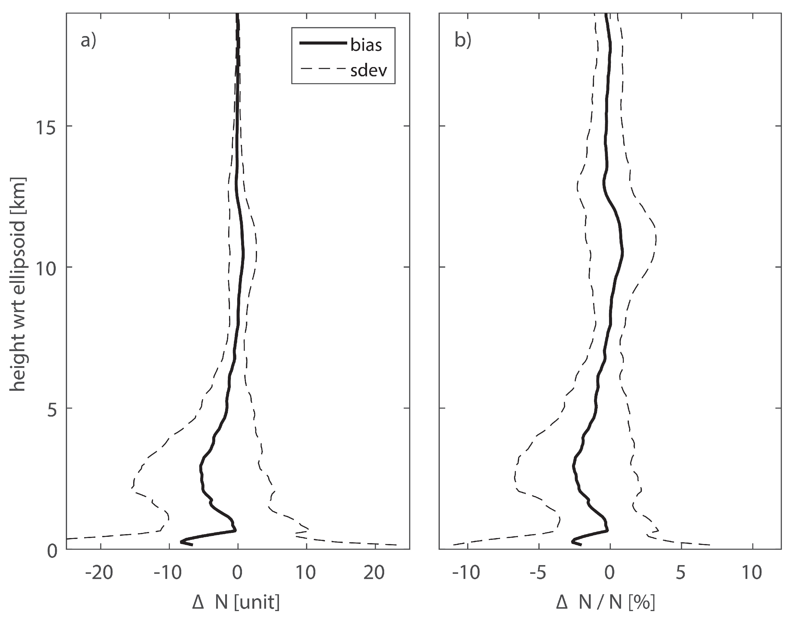
53]. The rainfall events were treated separately regarding to the rainfall intensity and analyzed for five different thresholds. Additionally, at one radiosonde location, central with respect to the area of interest, radiosonde minus WRF refracitivity fields were calculated for whole study period. Resampled differences in model space were used as an input for uncertainty propagation with ray-tracing.
6. WRF Model Evaluation
The model performance for the entire study period is summarized in
Table 3. The model underestimates observed air temperature and relative humidity at 2 m. Correlation coefficient exceeds 0.8 for air temperature, which suggests good temporal agreement between the model and observations. Cor is lower for relative humidity and wind speed.
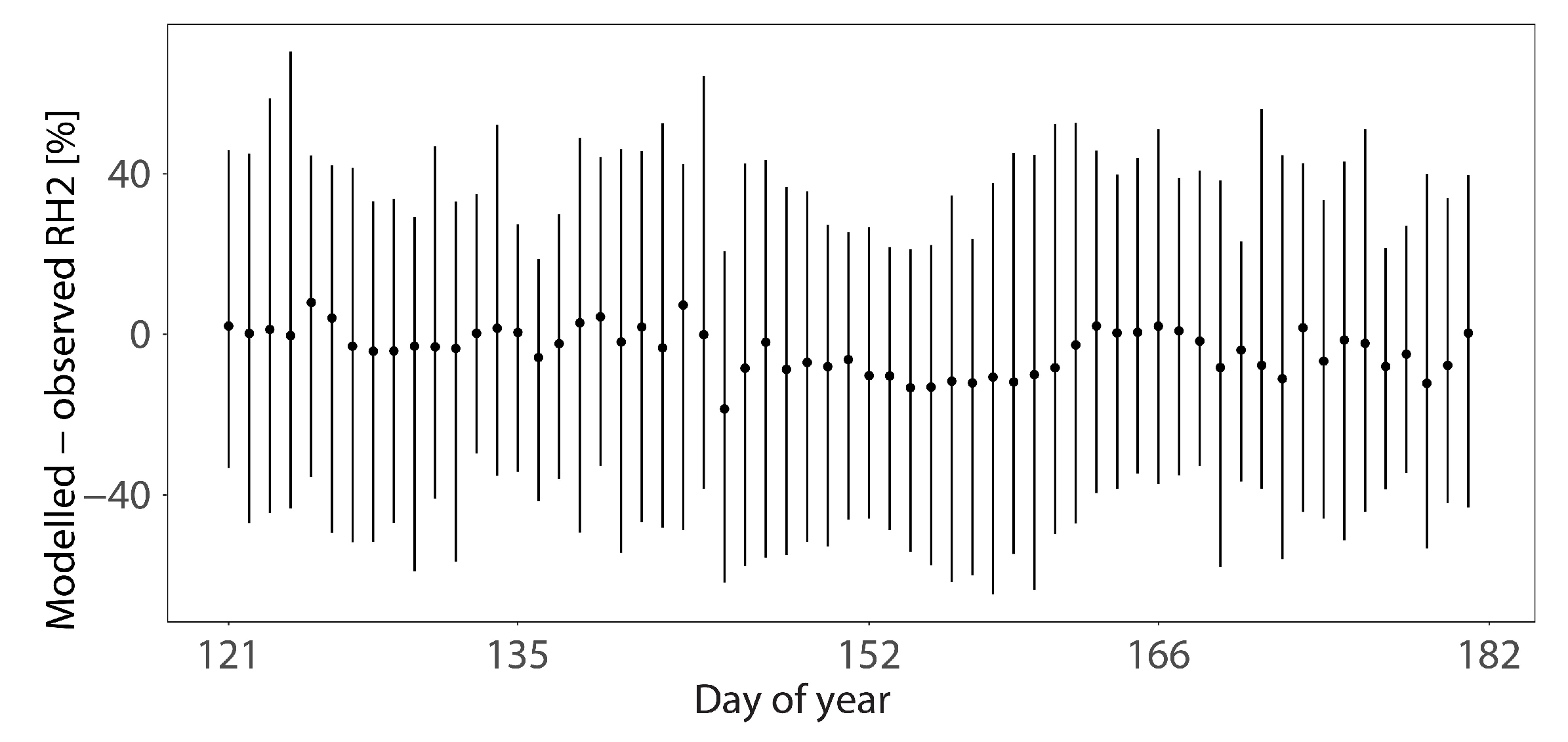
The changes in model performance during the study period is summarized for air temperature in
Figure 1 and relative humidity in
Figure 2. For air temperature, the model tends to underestimate the observed values during the entire period except the days from 152 to 162 DOY. For this period, the median values of the model-observation are significantly above zero. For the same period relative humidity is underestimated.
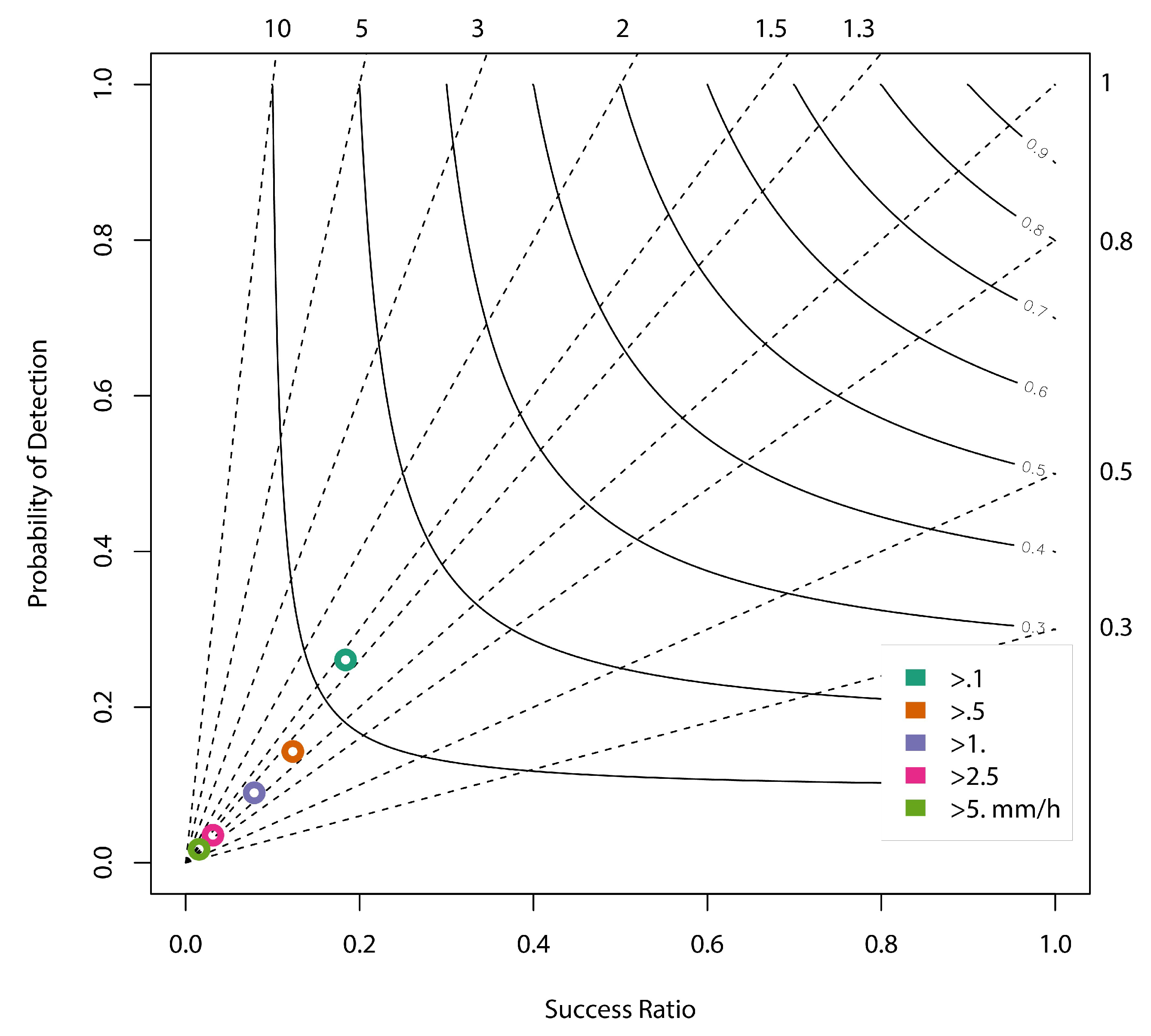
The model performance for rainfall is summarized in
Figure 3 using the binary evaluation. The model skills in forecasting rainfall decrease with observed rainfall intensity. This is partly because of the fact that the high intensity rainfall episodes are of convective origin and cover only small areas and are short in time. This, combined with high spatial and temporal resolution of the data (even relatively small shift in modeled rainfall location/time will lead to errors in binary evaluation) and small number of the episodes with high intensity of rainfall leads to poor performance of the model for the thresholds >2.5 mm/h.
The model performance for rainfall was also analyzed for each day of the study period. For each day the mean daily rainfall intensity was calculated from hourly measurements gathered at all stations and from corresponding WRF model grid cells (
Figure 4). The correlation between the modeled and measured values is high and close to 0.7. The model underpredicts the mean daily rainfall intensity for the peak days, but still, for the majority of days, shows increased values for the days with high measured intensity.
7. Cross-Validation of Ray-Traced and GNSS Slant Delays
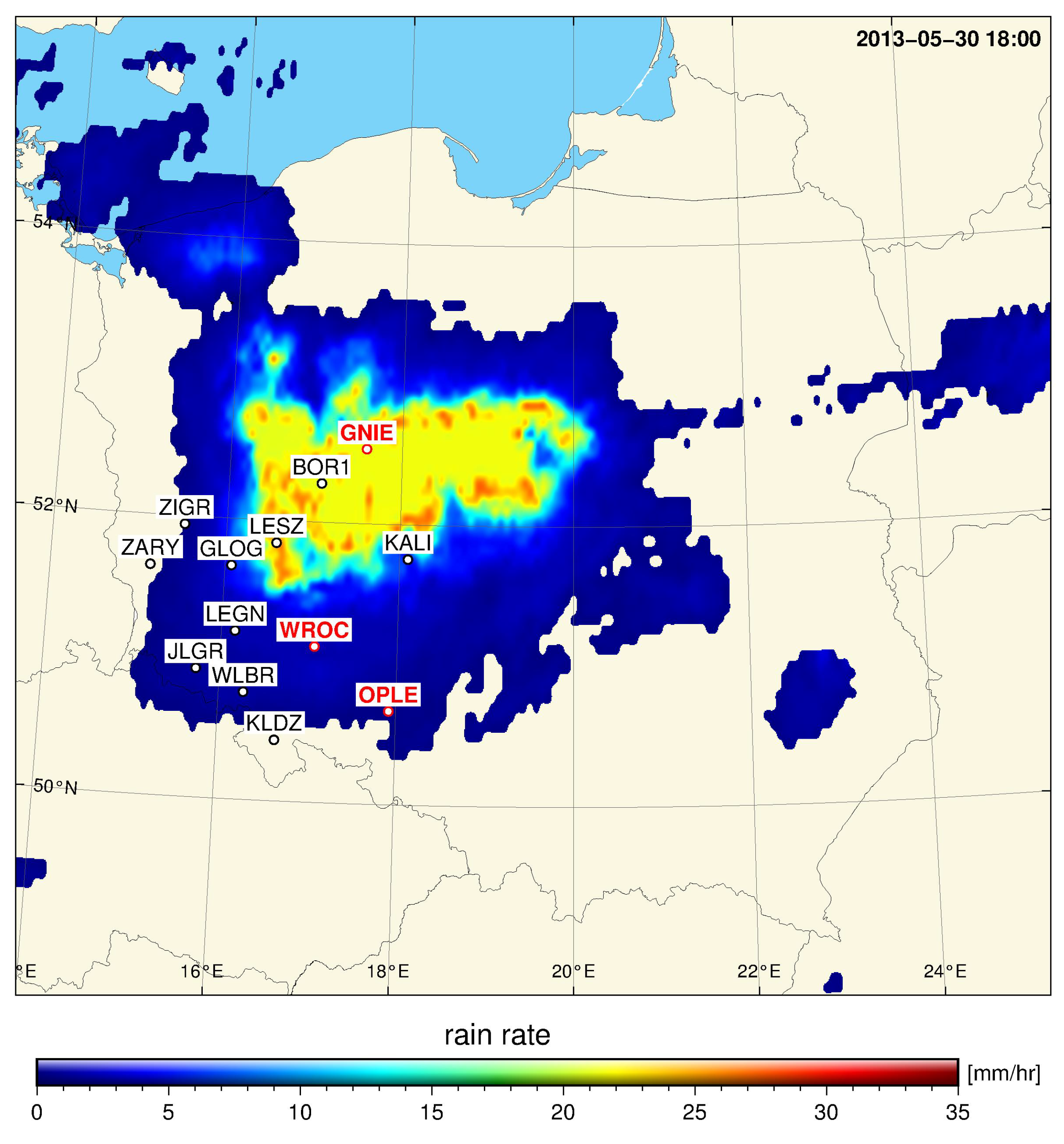
We analyze the quality of tropospheric delays based on representative sample of thirteen ground GNSS stations in southwest Poland that vary in altitude and location. Stations with following IDs of ASG-EUPOS network are considered: GLOG, GNIE, JLGR, KALI, KLDZ, LESZ, OPLE, WLBR, ZARY, ZIGR including three EUREF Permanent Network (EPN) stations: BOR1, GWWL, WROC.
Figure 5 displays the distribution of the station network. Table with listed GNSS stations and their coordinates is provided in
Appendix C. Collected GNSS observations cover a benchmark period of COST ES1206 GNSS4SWEC Action [
19] between 5th May and 30th June of 2013, which corresponds to 125 and 181 day of year (DOY). Selected stations belong to the PL0 cluster.
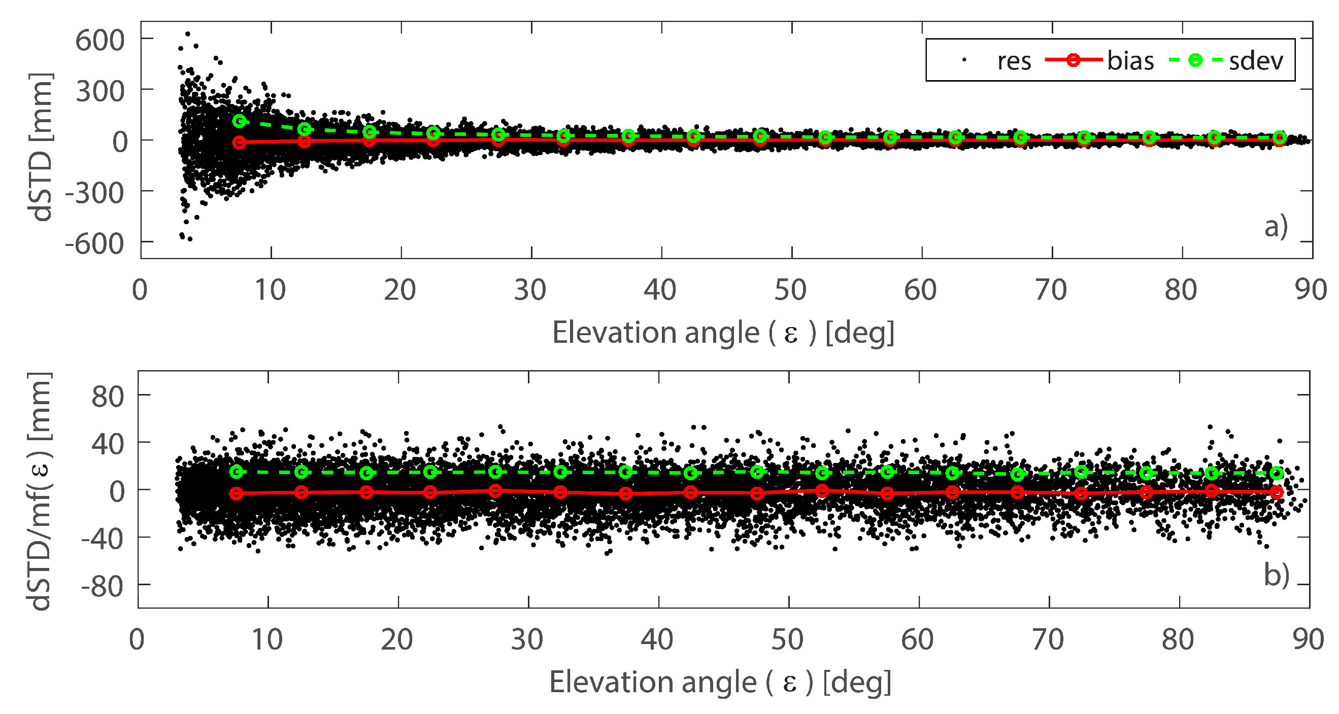
Slant delays down to three degree of elevation angle are taken into account to calculate residuals as GNSS minus ray-traced values in 1-h temporal resolution. A clear dependence on the elevation angle is displayed in
Figure 6a. The mean statistics respective for STD differences are calculated in 5-degree bins of elevation angle starting from 5 degrees up to 90 degrees. Slant delays below 5 degrees are not analyzed in terms of mean bias and standard deviation due to relatively low number of observations. Therefore,
Figure 6a shows that their residuals can reach up to 600 mm for 3 degree elevation angle. The results suggest no considerable differences in estimated STDs as an effect of applied GNSS processing scenario. The inconsistencies in terms of standard deviation due to neglected horizontal gradients equals only 3 mm. Although the reconstruction with horizontal gradients leads to more biased STDs towards smaller values, estimates at the lowest elevation angles are mostly affected. Additional 8 mm negative bias is observed below elevation angle of 5 degree. However, estimates at such low elevation angle are not used in the statistical assessment of hydrometeors’ contributions to tropospheric delays.
Since ray-traced and GNSS-based slant delays are calculated together with their respective mapping functions separated on hydrostatic and wet part, it is possible to express residuals in the zenith direction. ZTD discrepancies are presented in
Figure 6b. The differences generally do not exceed 50 mm, which is a valid residual distribution for STD differences at high elevation angles. No distinctive systematic effects with respect to the elevation angle are observed in ZTD residuals. The delays are affected by mean bias of around −2.5 mm and have 14 mm or 14.4 mm standard deviation, respectively for solution including and excluding post-fit residuals.
The results show that the quality of ray-traced delays with respect to GNSS estimates is comparable to the study of Kačmařík et al. [
17]. There is no statistically significant difference induced by a treatment of post-fit residuals in GNSS solution nor the horizontal gradients affect STD and ZTD values considerably. Therefore, the interpretation of results in the following study will be independent on the applied GNSS processing scenario.
9. Applications in Weather Monitoring
As stated in Kačmařík et al. [
17] and Solheim et al. [
18] the presence of hydrometeors should be visible in estimated GNSS tropospheric delays. In our initial study, we use ray-tracing to attribute the induced delay to the gaseous part of the troposphere by Equation (
2). Hence, the GNSS observations should differ from WRF delays by the neglected hydrometeors contribution assuming properly modeled atmospheric conditions. Part of the impact is expected to be introduced by small uncertainties originating from NWP model. However, this effect is kept to minimum by quality verification procedure using the error propagation and filtering of analyzed time-series. The theoretical impact of liquid water and rain rate on zenith delays is illustrated and described in
Appendix B.
The analysis of hydrometeors impact on GNSS signal propagation in terms of dependency of ZTD residuals on CT product is presented in
Figure 11. GNSS STDs estimated under specific cloudy conditions were selected from observations in 6-hourly temporal resolution, as provided by CT data. Corresponding ray-traced delays modeled in a cloud-free atmosphere were subtracted from GNSS observations to estimate potential cloud contributions. The differences calculated at 13 GNSS stations were mapped to the zenith to make troposphere delays independent on the elevation angle. Cloud type estimates from 15 pixels around each GNSS stations are subtracted from the MPE product and median value is calculated for each observation epoch (6 hours in case of CT). Mean dZTDs for each cloud class for all stations and epochs are calculated and displayed in
Figure 11. The CT ranges follow from
Table 1.
Results show that, on average for epochs with high content of clouds expressed by CT above 5, dZTD is consistently biased from 10 mm at station KALI up to 20 mm at station GNIE. Moreover, for the moderate cloud content, the magnitude of dZTD bias is lower, but still clearly pronounced. The variability from 6 to 12 mm is observed on the example of stations ZIGR and ZARY, respectively. Atmospheric conditions described by low CT values introduce either no bias or slight negative bias of −5 mm, with an exception of station OPLE where positive bias of 4 mm applies. For stations ZIGR, JLGR, BOR1, GLOG, LESZ, LEGN, GNIE, there is a clear, around 10 mm separation between cloud classes. The respective separation for stations KALI, OPLE, KLDZ, ZARY, WRIC, WLBR is lower by 3 mm, especially between class with high or moderate cloud content. It has to be noted however that for each CT class the spread of dZTDs measured as a standard deviation varies between 16 mm for CT below 3 to 20 mm for CT above 5.
Similar analysis is performed for rain rate intensity and its effect on GNSS tropospheric estimates. The dependency of ZTD differences on MPE product results is summarized in
Figure 12. ZTD differences are grouped into three classes for respective MPE: (1) affected by rain intensity under 0.01 mm/h; (2) light rain between 0.01 mm/h and 2.5 mm/h; (3) significant precipitation over 2.5 mm/h. Similar pattern, as for CT product, could be observed. The localized rain events are however less frequent than analyzed cloudy conditions. The number of observations within each class varies and cases of minor precipitation under 0.01 mm/h are the most frequent, resulting in over 700 observations. Light rain affected 50 observations, whereas for the significant rain only up to 15 cases at each station were found. Hence, respective data samples are not equally representative.
Recent study on the MPE quality [
57] based on ground-based rain gauges shows that for light rain with intensity below 5 mm/day the MPE retrieval might not agree well with the rain gauge data (0% events detected). Better performance is provided for the medium rain rates (5–20 mm/day) with only 31% events undetected. High detection rate applies to extreme events with precipitation above 20 mm/day with only 10% undetected. Therefore, the emphasis is put on analysis of tropospheric delays in cases of heavy precipitation. The results presented in
Figure 12 prove that tropospheric delays affected by low precipitation events introduce significantly smaller bias than rainfalls of medium or high intensity. Station JLGR is the only example that does not follow this rule. The dZTD bias for low rain class varies between 4 mm and 8 mm and is always positive. 7 out of 13 stations investigated have greater dZTD bias for intensive rain events, where precipitation varies from 2.6 mm/h to 22.9 mm/h, than for medium rain from 0.1 mm/h to 2.5 mm/h. According to
Figure 12, the separation between rain and no-rain events expressed as a mean ZTD difference is between 12 and 18 mm. It has to be however noted that for each MPE class the spread of dZTDs measured as a standard deviation is between 20 mm for no rain class to 16 mm for highest rain intensity.
The analysis of hydrometeors impact on discrepancies in tropospheric delays from GNSS and ray-tracing is summarized in
Table 4 by correlation coefficients with respect to CT and MPE products. The correlation between CT and ZTD differences is always positive and reaches up to 0.43 at station JLGR. This suggests that the cloud coverage could affect GNSS observations. The average correlation for CT is at the order of 0.38. Therefore, larger CT parameter introduces increments in ZTD discrepancies between GNSS and ray-tracing. The correlation coefficients for MPE product indicate similar relationship of ZTD differences as for CT product. The increase of MPE at 8 out of 13 stations (OPLE, KALI, WROC, GNIE, KLDZ, ZIGR, BOR1, LEGN) is related to the significant increase of correlation coefficients. If MPE > 0.01 mm/h is considered, the average correlation
is 0.10. For MPE > 2.50 mm/h the increment in the correlation coefficient yields 0.28. However, negative correlation coefficients with respect to MPE can be also identified in
Table 4. One of factors that might contribute to such incidences is a non-uniform representation of ZTD differences within MPE ranges for concerned stations. The coefficients can be also affected by sampling errors arising from uneven data series, though cannot entirely explain such large uncorrelation. Particularly, the lack of correlation coefficient for JLGR is due to the low number of observations with MPE > 2.50 in the vicinity of the station.
The applied approach within this study disables a direct separation of hydrometeors on the rain-induced (MPE product) and cloud cover (CT product) contributions to GNSS tropospheric delays. However, the impact of typically negligible terms of atmospheric refraction is observed in the statistical sense. The larger contributions to the delays are expected due to a significant cloud cover rather than those induced by precipitation events. This suggests that severe weather events could be considered in the analysis of GNSS data time-series as a source of larger tropospheric delays. The ability to isolate the impact of weather events demonstrated by the analysis of GNSS and ray-traced data can be further studied based on GNSS observations co-located with water vapor radiometers, radars and in-situ rain gauges to support presented results.
10. Discussion
The number of research papers that deal with the impact of intense weather events on GNSS tropospheric delays is still low. One of the first attempts to assess effects of hydrometeors on GNSS signal was a paper of Solheim et al. [
18]. The authors estimated delays due to permittivity of ice and water droplets sustained in clouds to 8 mm/km, which contributes with 40 mm to the delay if we assume 5 km constant liquid and ice concentration in the zenith direction. The propagation delay due to scattering induced by rain can reach 6 mm, assuming the signal travels through 3 km in the presence of rain with 20 mm/h rate. Such semi-empirical estimates agrees with the results of our study showing biases up to 45 mm (
Figure 10). Moreover, stations with large amount of water and ice in the clouds (above class 5) or rain detected by MPE algorithm show consistent mean positive bias through the whole Benchmark campaign period with average biases of up to 25 mm as indicated in
Figure 11 and
Figure 12. This bias, however only slightly exceeds the standard deviation of collected dZTD, which varies between 16 mm and 20 mm, and hence more data in each class are required in further studies. Also comparing the RH in
Figure 2 and rain intensity in
Figure 4 between day 135 and 166, one can see that more rain (quite well captured by the model), leads to increased negative bias of RH, which means that the model underestimates the water vapour. It may result in increased difference between GNSS and the model. The initial physics-based retrieval of liquid and rain rate induced delay illustrated in
Figure A2 suggests that hydrometeors do not introduce delay exceeding 5 mm. However, these calculations are based on forecast variables and MPE rain rates that depend on the performance of individual background data, which might require further verification.
De Haan et al. [
20] presented azimuthal anisotropy of the atmosphere from GNSS and NWP data during a cold front passage. The SWD gradient varied by 40 mm and helped to indicate boundary of investigated event. The variability is also demonstrated in the following study as there are differences between stations in mountain valleys (JLGR) and low-lands (WROC). Brenot et al. [
21] tested sensitivity of GNSS observations collected during weather event that brought an intense precipitation. GNSS ZTDs were compared with corresponding delays from NWP model that attained sporadic hydrometeor contributions up to 70 mm. Kačmařík et al. [
17] and Douša et al. [
19] estimated maximum hydrometeor contribution of 17 mm in zenith direction during extreme weather events, whereas observations in this paper showed mean ZTD discrepancies at the order of 10 to 30 mm.
Currently, there are no tools available in widely used Bernese GNSS Software [
34] to improve the GNSS tropospheric delay estimation under unusual weather conditions. Thus, no sophisticated processing strategies are applied for GNSS products retrieval under intense weather events [
19] which are mostly limited to data constraining. In most geodetic applications, the atmosphere is assumed to be calm [
28,
58]. Due to the magnitude of the liquid and ice water that is relatively small, their impact is also considered to be negligible when applying ray-tracing methods [
13,
14,
27]. The mismodeling effect of conventional gradient model [
26] in GNSS processing has been already indicated by [
25] and proves that major change in the functional model for troposphere estimation is required. The estimation procedure could be also improved by adding satellite-grade clock to the receiver to remove one estimation parameter. Another approach is to observe the same satellite with at least three collocated receivers (three degrees of freedom more). Certainly, the application of new method for gradients, as reported by [
25], is a step forward.
Further verification of impact of hydrometeors in a case-by-case study requires high quality NWP data an input for ray-tracer. Data from instruments that can directly derive the liquid and ice water content along line-of-sight between a satellite and a receiver are essential source for the purpose of validations. Microwave radiometers and other devices to measure cloud base height e.g., ceilometer should be considered. An effort should be made towards inter-comparisons of GNSS and ray-traced slant delays with included hydrometeors, which would influence the current level of inconsistency and help to improve predictions of rain- and cloud-related variables in NWP models. The residual time-series should be carefully analyzed in order to distinguish between the noise and potential systematic effects associated with atmospheric conditions. The application of multi-GNSS data [
59] is likely to lower uncertainty of final solution, hence providing better estimates of tropospheric delays. Since the higher the intensity of weather events, the higher contributions of the liquid and ice water on GNSS signal is expected. Thus, it is recommended to use examples of tropical cyclones and mesoscale convective systems for case studies.
11. Conclusions
GNSS observations are commonly recognized by all-weather capability, thus allowing to continuously monitor weather conditions. The troposphere-induced delays are highly dependent on atmospheric conditions and their magnitudes can be used to express intensity of weather phenomena. The presented study focuses on higher order terms of tropospheric refractivity and their contribution to GNSS estimates. Based on the observations collected during intense rainfalls and cloudy conditions, the effect of associated liquid and solid water terms is expected to affect tropospheric delays. The assessment of such dependency is performed based on retrievals of STD from GNSS observations and ray-tracing technique. The ray-traced delays contain contribution of NWP-based gaseous constituents. The GNSS signal propagates through the real atmosphere and contains contribution from all atmosphere constituents. The difference was assumed to give the rain and cloud impact. To avoid and account for NWP-induced errors, the uncertainty analysis was performed for NWP refractivity field with respect to radiosonde observations and for GNSS slant delay estimation process. Epochs with combined uncertainty of ZTD larger than the mean error of 5.2 mm were removed from further investigations to ensure robust interpretation of the results.
By comparing GNSS and ray-traced tropospheric delays, we were able to estimate the tropospheric delay precision. In the zenith direction, delays agree to within −2.5 mm in terms of bias and 14 mm in terms of standard deviation. Various processing strategies of GNSS observations were applied in order to account for signatures induced by clouds and rainfalls. Results, however, presented only negligible differences in terms of bias and standard deviation for analyzed processing scenarios when compared to ray-traced delays. Treatment of post-fit residuals and application of horizontal gradients from GNSS solution is showed to play a minor role in the estimation procedure. This suggests that ZTD estimation algorithms, with one correction for all satellites, only two gradients and residuals, are not fully representing slant delays.
In the analysis of hydrometeors impact on tropospheric delays, over 131,000 slant delays were considered at 13 stations. The data sample was composed of GNSS observations in cloudy and rain conditions expressed by CT and MPE remote sensing products, respectively. Positive ZTD residuals were indicated for observations that propagated through thick clouds and intense rain. The introduced systematic effect varies between 10 to 30 mm, whereas standard deviation for obtained values varies between 16 and 20 mm. The differences are correlated with intensities of phenomena since more significant clouds and precipitation rates lead to increments in correlation coefficients. ZTD discrepancies are lower for CT parameter than for MPE product. However, separation of GNSS observations characterized by different magnitude of precipitation is less pronounced for precipitation rates. This might be due to more localized rainfall events relative to cloud, which tend to form more extensive fractions.
The initial model-based liquid water and MPE rain rates retrieval shows maximum impact of hydrometeors to be on the level of 5 mm. However, to further advance this research, ray-tracing algorithms should be augmented with liquid water contributions associated with severe weather events to independently assess their magnitude. NWP models need to be carefully validated against radar, radiometer or satellite observations in order to establish comparable data-set, distinguish the effect of hydrometeors and to investigate the impact of estimation procedure on the inhomogeneity studies. The emphasis should be placed on better recognition of azimuthal anisotropy so that weather events could be robustly localized based on differences in tropospheric delays.


