1. Introduction
Antarctica is an important area due to its ongoing glaciation and contemporary climate-driven rapid changes. Geodetic and geophysical observations on Holocene changes in Antarctica will give us unique information when studying global climate-change related phenomena. Long time series of geodetic and geophysical stations provide data explaining parts of the interaction between solid earth, cryosphere, hydrosphere and atmosphere. They are also essential as ground truth when data from satellite missions are analysed.
Finland joined the Antarctic Treaty in 1984, became consultative party in 1989 and full member of the Scientific Committee on Antarctic Research (SCAR) in 1990 [
1,
2]. Five years later after signing the treaty, the Finnish research station, Aboa, was established in Dronning Maud Land (DML), East Antarctica. All Aboa activities were gathered under the general heading of the Finnish Antarctic Research Program (FINNARP). The first FINNARP expedition took place during the Antarctic summer of 89/90. Since then, a total number of 26 FINNARP expeditions have been arranged during the Antarctic summers (
http://www.antarctica.fi/). There were no expeditions during the summers of 90/91, 94/95, 96/97 and 98/99. The research activities associated with the expeditions have been mainly financed by the Academy of Finland via regular calls for Antarctic research issued every fourth year. In addition, universities and research institutions invest financial resources of their own for Antarctic research [
2].
In recent years, the Finnish Antarctic research has focused on geodesy [
3,
4,
5], glaciology [
6,
7,
8], geology and geophysics [
9,
10,
11,
12,
13], air quality and climate change [
14,
15,
16,
17,
18], meteorological and space physics [
19,
20,
21,
22], marine and structural technology [
23,
24], oceanography and marine biology [
25,
26]. Typically, the research work has been undertaken at Aboa and surrounding areas. These research activities have sometimes been complemented with trips and overnight stays to more distant locations, including the coast. In addition, foreign researchers have participated in the FINNARP expeditions and Finnish researchers have worked at foreign research stations and on board of foreign vessels. For example, Finnish researchers have performed ozone and ultraviolet (UV) research at the Argentine Marambio research station, cosmic rays research at the Italian-French Dome Concordia station, or marine and sea-ice research on South African R/V Agulhas II. Absolute and relative gravity measurements have been done at the Norwegian Troll station, Russian Novolazarevskaya station, Indian Maitri station, and South African SANAE IV station. SCAR GPS measuring campaigns have been conducted at several locations, including Swedish Wasa station neighbouring Aboa. Furthermore, logistic and research support has been provided to international collaborators, e.g., satellite controlled meteorological balloons on behalf of the Smith College, USA (
http://www.antarctica.fi/).
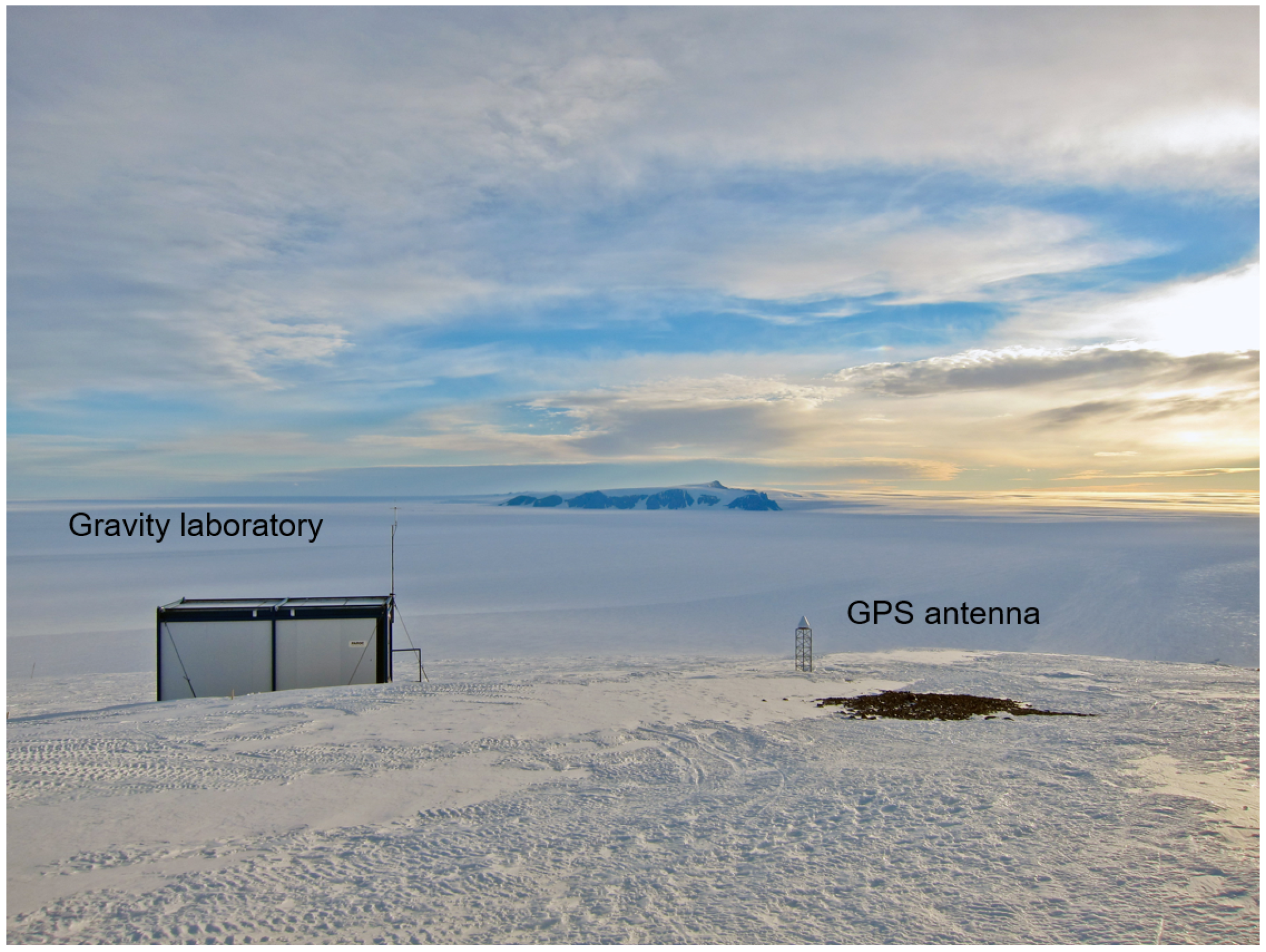
Currently, the Aboa research station is equipped with several automated year-round measuring instruments, such as continuous GPS tracking equipment (2003), an automatic weather station (2004), and an automatic seismometre (2007). In addition, Finnish researchers have deployed other automated year-round measuring instruments outside Aboa, such as automated weather stations at the top of the Basen nunatak and near the coast, automated buoy at sea to measure the vertical temperature profile of sea ice, and cosmic ray detectors. All these measuring instruments ensure the collection of significant sample series and the continuation of long-term time series data in accordance with Finland’s Antarctic research strategy [
2].
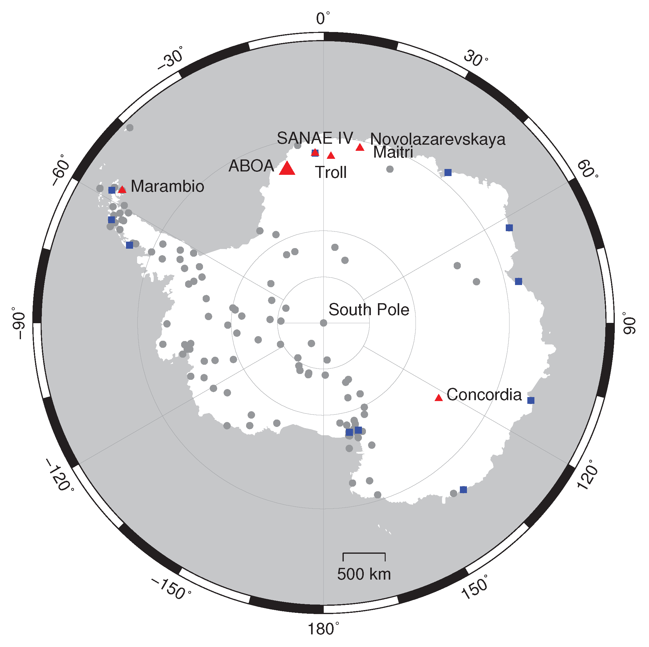
Numerous GPS and/or GNSS (Global Navigation Satellite System) continuous and episodic stations have been established in Antarctica in the last two decades (
Figure 1). The development has lead to GPS becoming an essential component of geophysical and meteorological research for studying fundamental solid Earth and atmospheric processes that drive natural hazards, weather, and climate [
27]. The first GPS measurements in Antarctica were conducted in the early 90s. The main objective was to gain detailed insights into the tectonic behaviour of the Antarctic plate [
28,
29]. The accumulation of the measurements allowed the definition of a precise reference frame [
30]. Later, Thomas et al. [
5] analysed GPS data from more than 50 stations across Antarctica. The authors estimated a more complete and precise vertical velocity field that allowed them to observe increase in uplift rates in the northern Antarctic peninsula after 2002–2003. Plate tectonics and vertical deformation studies also triggered the development of local or regional-scale projects [
31,
32]. Long time series of continuous GPS data have been used to constrain and test the reliability of glacial isostatic adjustment (GIA) models [
33,
34,
35]. Furthermore, GPS measurements in Antarctica have allowed atmospheric studies, such as ionospheric scintillation [
36,
37] or ground-based water vapour retrieval [
38,
39].
Aboa is an important GPS station in Antarctica due to the sparsity of bedrock sites, especially in East Antarctica. As seen in
Figure 1, most of the sites are located in West Antarctica, whereas the number of sites is much lower in East Antarctica. In addition, the distances between the sites are rather large and limited to coastal regions of the continent where bedrock can be found. Furthermore, only a limited number of sites provide continuous GPS observations. As of 26 October 2018 (
http://www.igs.org/network), there are only 13 active permanent International GNSS Service (IGS) stations [
40] on the Antarctic continent and only 10 of them have longer continuous time series than Aboa. This study covers a time span of 15 years. This is two times longer than in [
5] who used data for 1959 days between 2003 and 2010, whereas [
42,
43] used reduced time periods. [
42] covered a period of 1415 days between 2009 and 2013, while [
43] analysed a time series derived for the 2010–2013 period. Furthermore, [
33] computed a series of theoretical expected site velocity uncertainty for 5, 10, and 20-year long time series. Their computations show that the uncertainty decreases with the length of time series. Therefore, our results have the benefit of longer time series and thus higher reliability. Our study is the first to include an in-depth analysis of all available Aboa GPS data.
The rest of the paper is as follows.
Section 2 describes the material and methods used to generate and analyse the coordinates time series.
Section 3 reports the numerical results of our study.
Section 4 discusses the obtained results and their relationship with other published data.
Section 5 summarises the main achievements, the importance of our study and the way how our work will continue.
3. Results
3.1. PPP-Derived Coordinate Time Series
This section reports on the quality of the PPP-derived coordinate time series at Aboa in terms of internal precision, accuracy and postfit observation residuals.
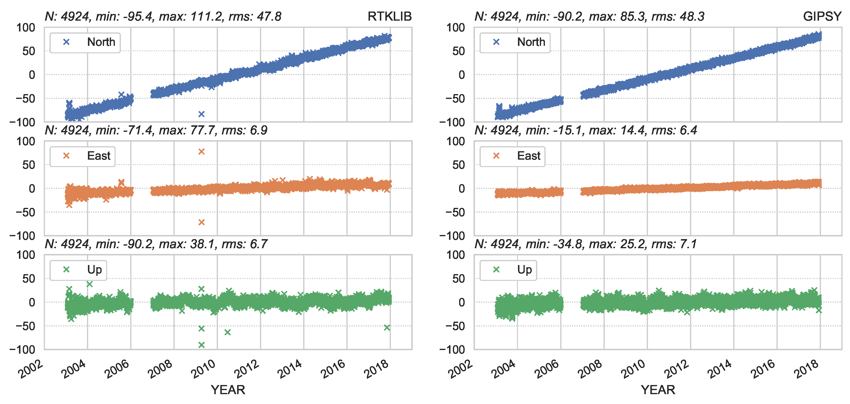
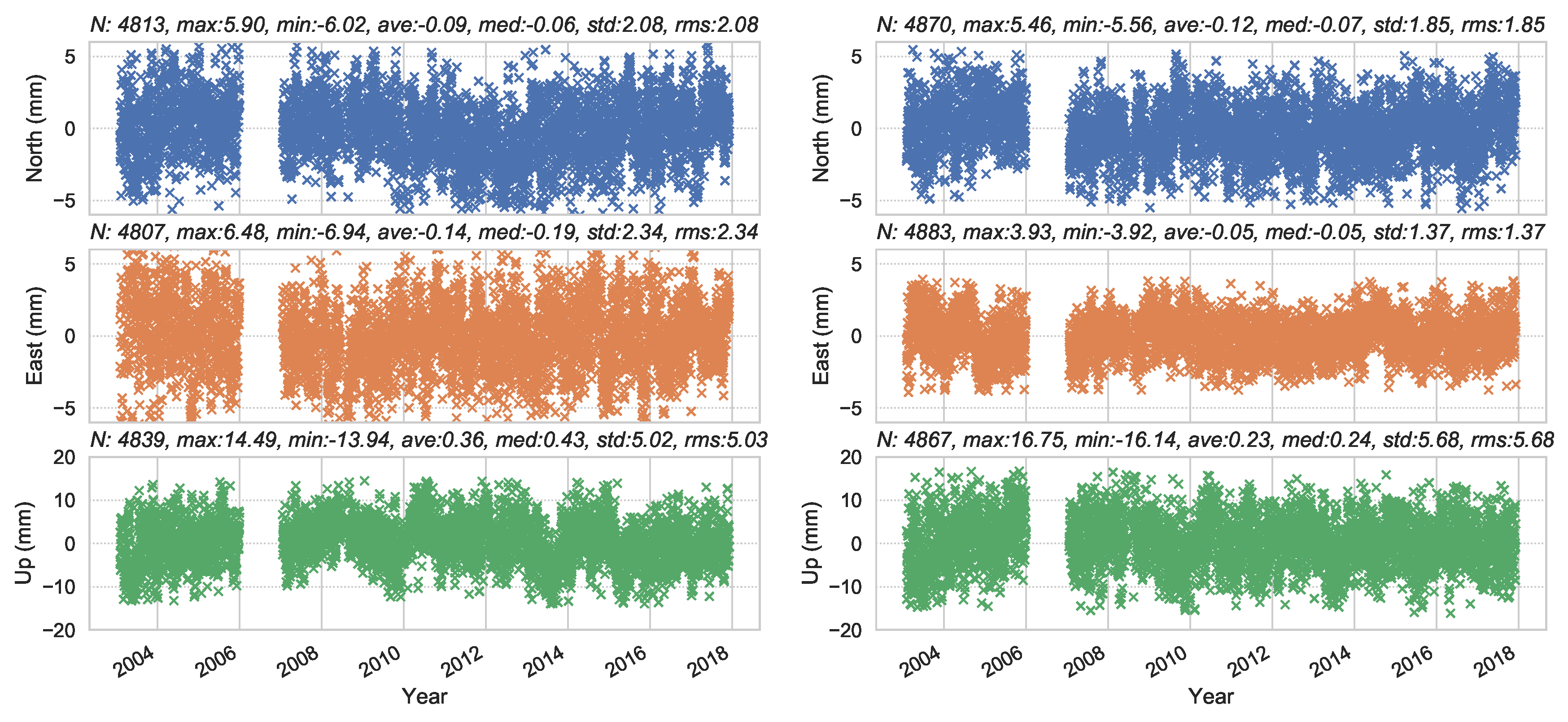
Figure 7 illustrates the topocentric coordinate time series at Aboa from the RTKLIB and GIPSY processing, respectively. The origin of the topocentric system is set to the mean coordinates over the entire period. Whereas the GIPSY solution shows no noticeable outlier, the RTKLIB solution exhibits a few obvious outliers. In addition, the RTKLIB solution appears somehow noisier. Nevertheless, both time series appear to follow a similar trend.
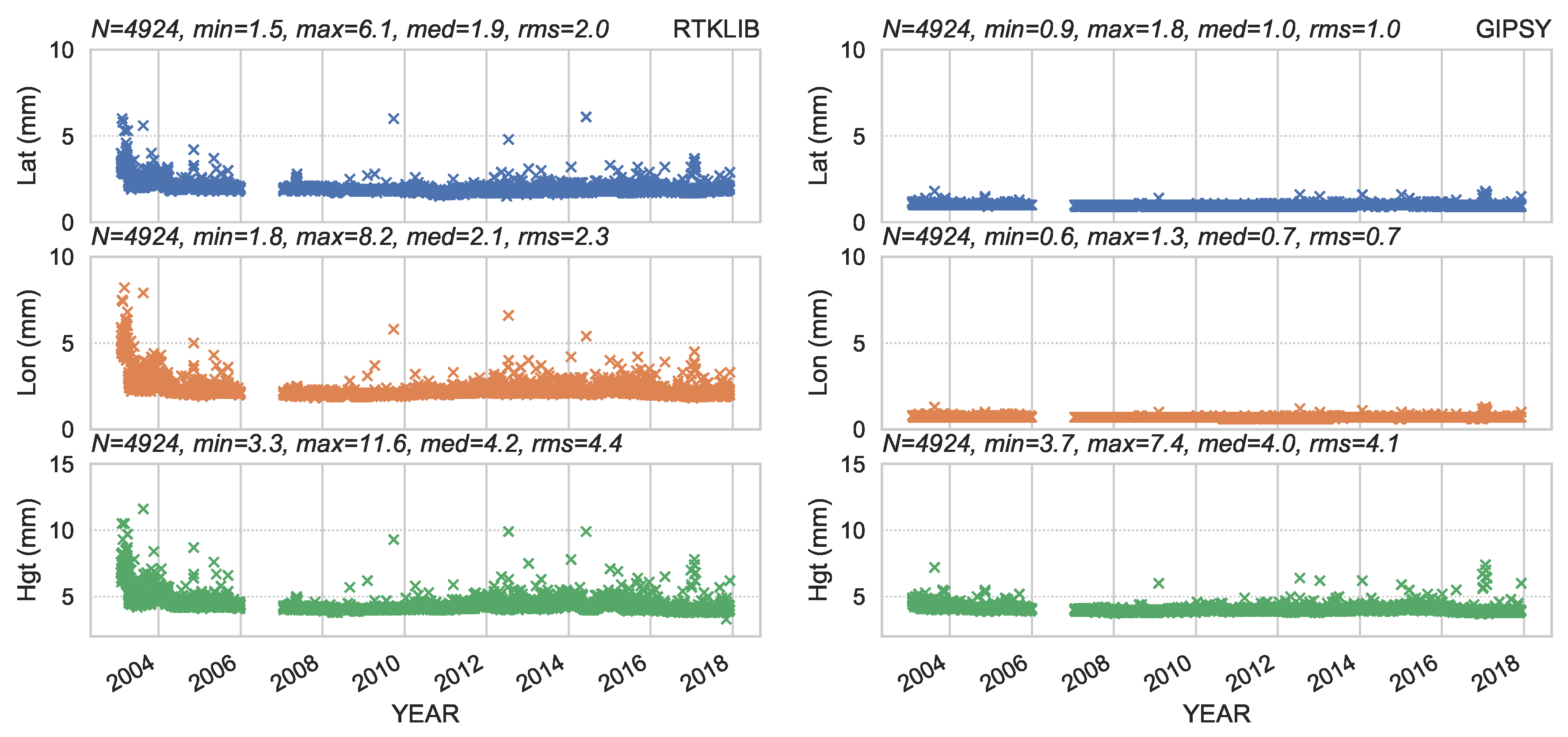
Figure 8 depicts the standard deviation of the estimated position as given by the processing engine. The median standard deviation along all the directions is below 5 mm. In the horizontal direction, the median precision is around 2 mm for RTKLIB and less than 1 mm for the GIPSY solution, respectively. In the vertical direction, both solutions exhibit about 4 mm median standard deviation. The GIPSY solution appears a little more robust for the entire interval period, whereas the RTKLIB solution exhibits larger standard deviations in the beginning of the time series. A significant improvement is visible in 2004. However, this may not be attributed to the processing engine but perhaps to the data quality or the difference in the precise products used by the two solutions. One may suspect a weaker performance of the products, perhaps in the Antarctic region, before April 2004. After that, the standard deviations appear rather consistent despite episodic mild jumps for a few days. Although these small differences, we can conclude that both time series are robust.
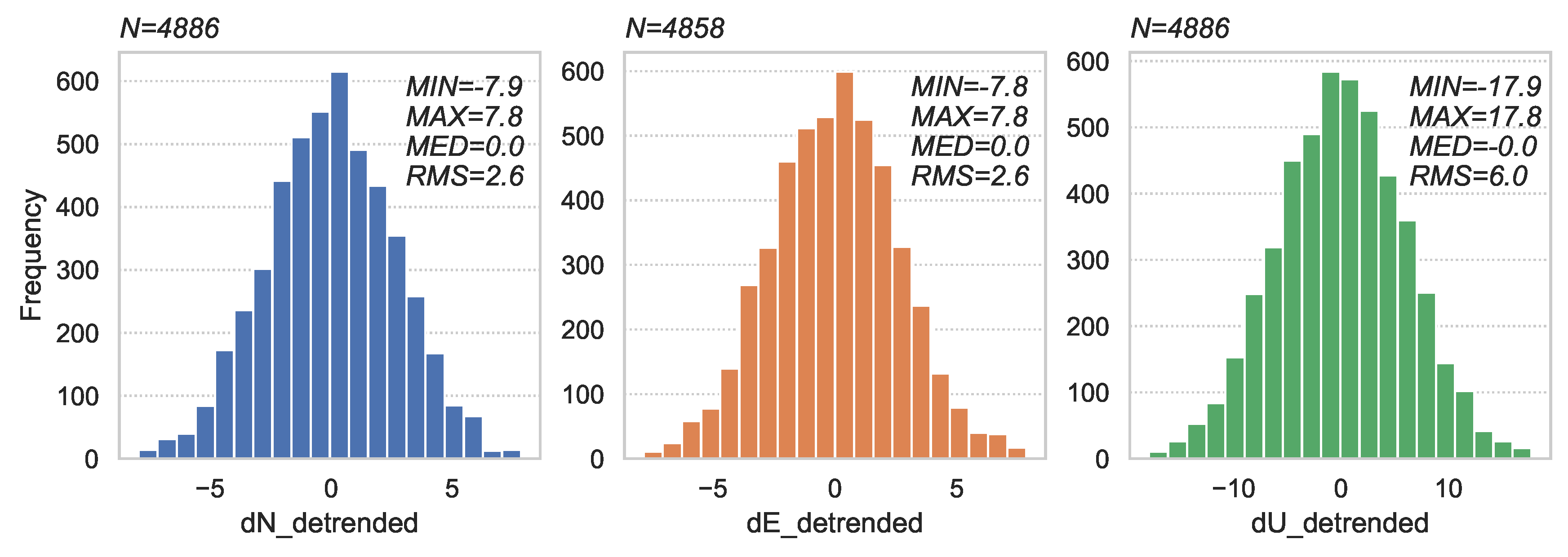
Figure 9 illustrates the accuracy of the RTKLIB solution with respect to the GIPSY solution as error distribution histograms of the local offsets. The accuracy validation requires that both series are expressed in the same frame. Thus, the RTKLIB coordinates were first transformed from ITRF2008 to ITRF2014. Then, the differences in Cartesian coordinates were calculated. These differences were converted to local NEU offsets for a more meaningful interpretation. Next, the outliers and trend were removed using a reiterative linear regression algorithm combined with the IQR (inter quartile range) robust statistic and a threshold of 2.2 for outlier removal. This threshold is roughly equivalent to the 3-sigma and it works well in our experiences. This process was carried out individually for each axis. The detrended offsets show peak-to-peak variations of less than ±8 mm for the North and East directions. The variations on the Up direction are twice as large and account for ±18 mm. Overall, 2.6 mm rms (root mean square) is obtained along the horizontal directions, whereas 6.0 mm rms is computed for the vertical direction.
Table 4 summarises the conventional and robust statistics. These statistics confirm an excellent agreement between the two solutions.
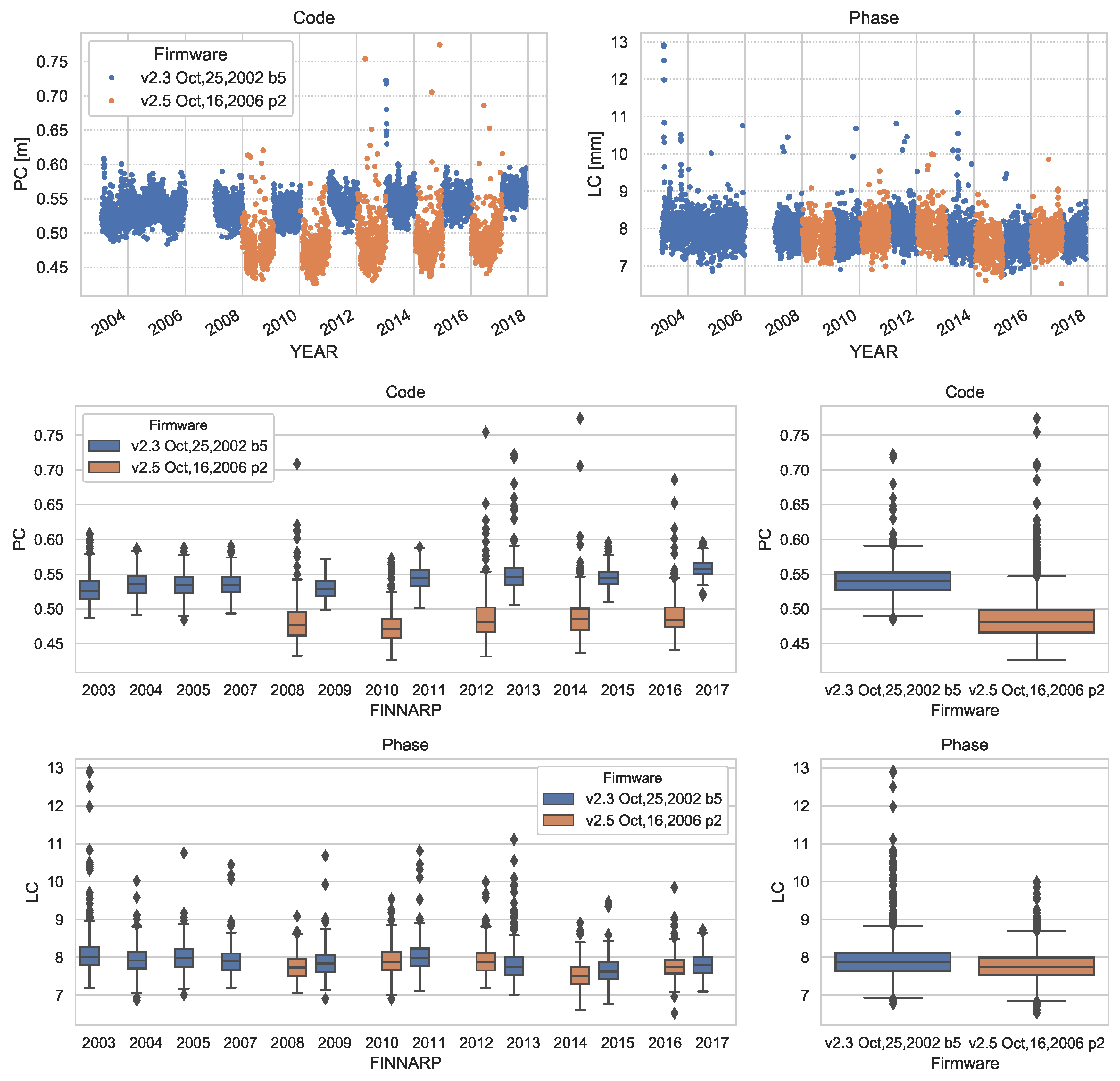
Figure 10 shows the code and phase observation post-fit observation residuals as obtained from GIPSY processing. The code residuals indicate a dual behaviour over time. This comes from the usage of two receivers mentioned in
Section 2.1. The receivers have been switched during the yearly FINNARP expedition, usually at year end/start.
3.2. Time Series Analysis
It is generally accepted that the GPS coordinate time series contain some form of temporally correlated noise along the expected white noise [
33]. The effect of this noise has direct effect on the uncertainty of the estimated parameters. We used Hector [
67] software that enables modelling the temporal correlation of the data and thus providing more realistic uncertainty estimates.
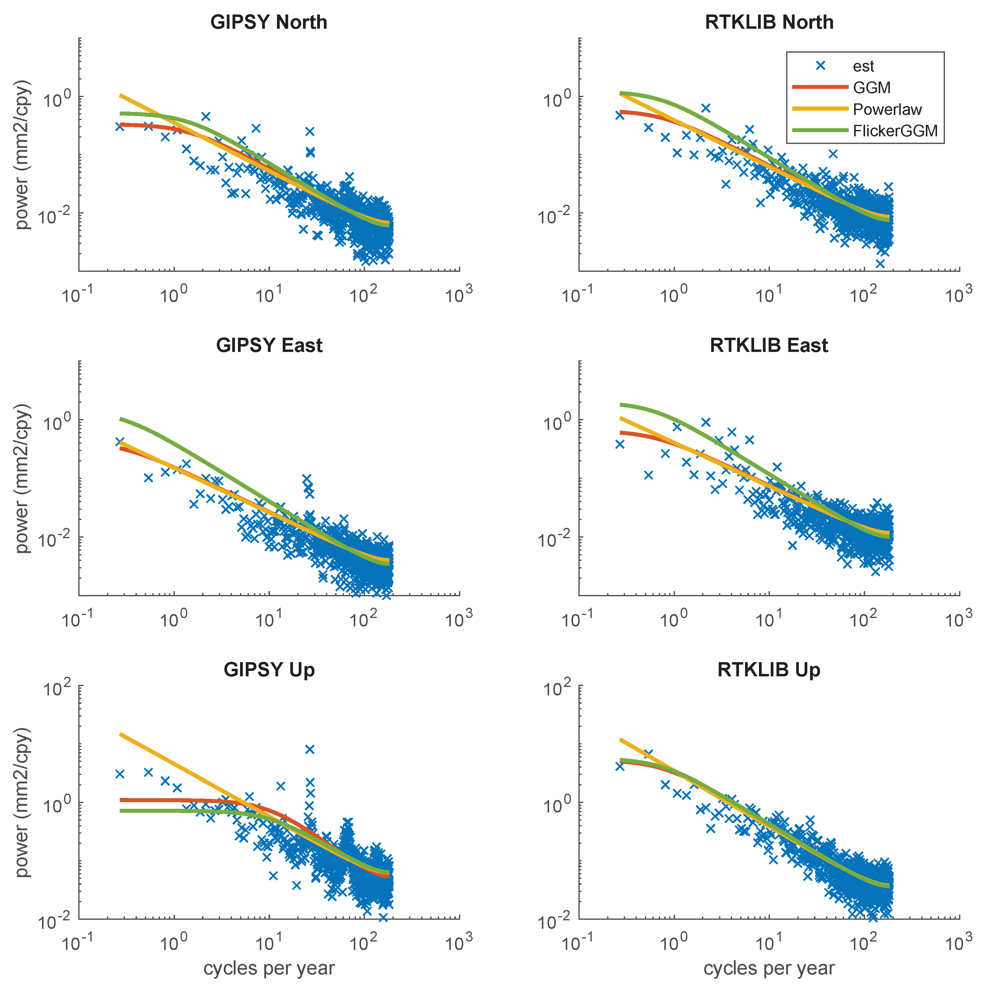
First, daily Cartesian coordinate time series were converted to local NEU coordinates with respect to the mean position, and the time series of each component was analysed separately. We found only one discontinuity in the time series analysis. It was linked to the switch from IGb08 to IGS14 in CODE’s operational solutions, which were used for the RTKLIB solution. Therefore, we solved an offset in the case of RTKLIB time series at 29 January 2017. The frame of the JPL products (used in the GIPSY solution) was the same for the entire period of the time series. Second, we removed the outliers using an IQR factor of 2.2. In addition, the offsets as well as annual and semiannual effects were taken into account in the outlier rejection. About 50 epochs (i.e., 1%) were rejected from the GIPSY solution and 100 epochs (i.e., 2%) from the RTKLIB solution, respectively. Third, we estimated the trends using three different noise models: Generalised Gauss-Markov (GGM), power-law (PL) and flicker noise implementation of the Hector (FlickerGGM). Typically, the white noise is added to the model, but in our time series the fraction for white noise was zero and, therefore, it was omitted from the model. The choice of the final model was based on the analysis of the power spectral analysis (PSD) and the Akaike and Bayesian information criteria (AIC/BIC). The model with lowest AIC or BIC values should fit best the time series.
Figure 11 depicts the PSD plots, whereas
Table 5 and
Table 6 summarise the AIC/BIC values. The results suggest that the GGM and PL models fit mostly equally best to the estimated spectrum. For the GIPSY Up component, the AIC/BIC analysis supports more GGM model, but the PSD plot shows that none of the model fits very well to the data. There are a few power peaks at roughly 27 cpy and 60–70 cpy corresponding roughly 14 and 5 day cycle, respectively. Those peaks probably cause the misfit of the models to the estimated spectrum.
Aboa coordinate time series contain temporally correlated coloured noise which spectral index is closer to flicker noise. The noise of the horizontal components is characterised by an average spectral index and average amplitude of 5 mm/y, whereas the noise of the vertical component has similar nature but three times larger amplitude, i.e. 16 mm/y.
Figure 12 depicts the coordinate residuals after removing the outliers, trend, annual and semiannual periodic signals. The rms error is reduced to less than 2 mm for the horizontal components and below 6 mm for the vertical component.
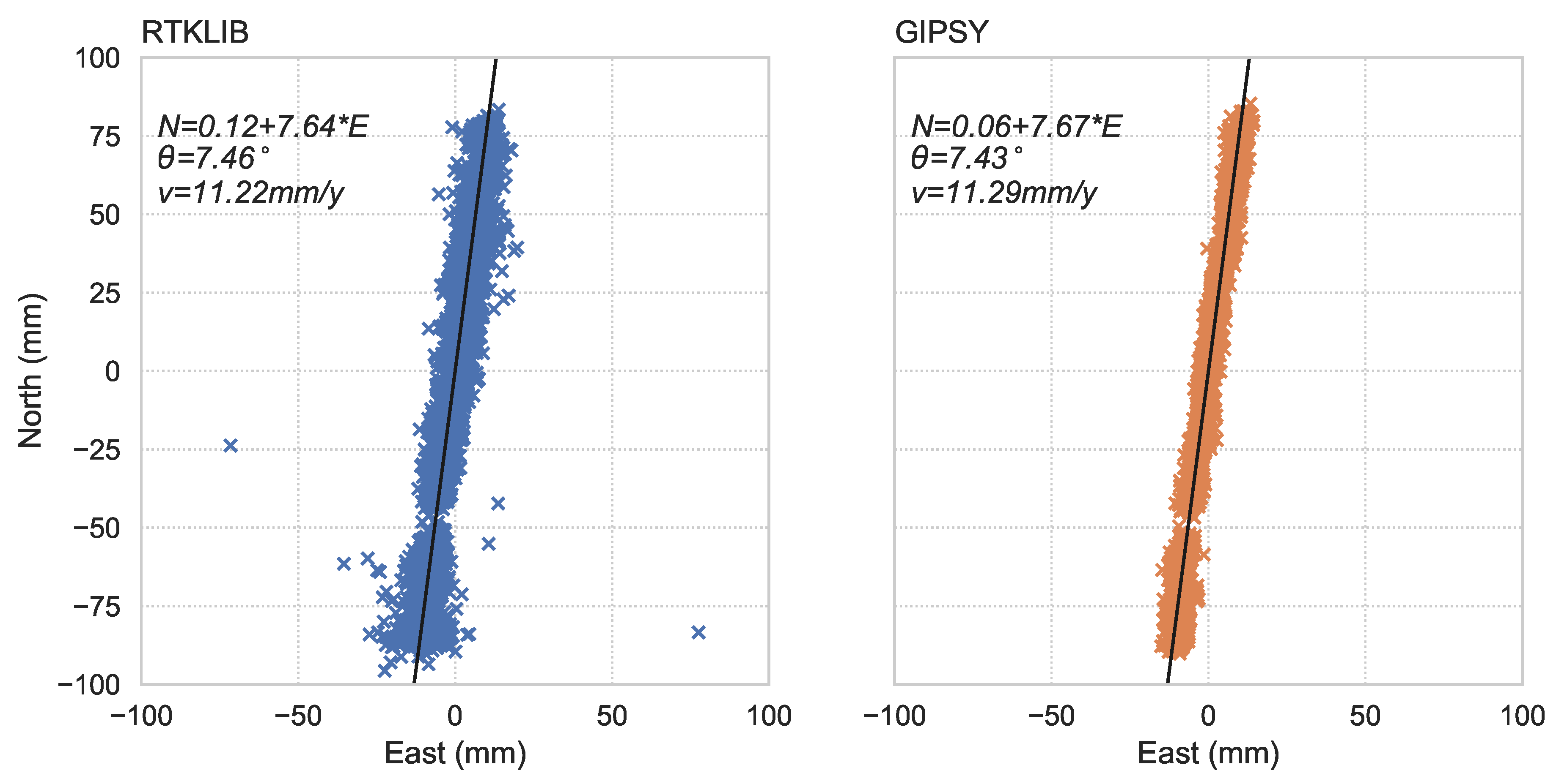
Figure 13 displays the horizontal movement. Since the beginning of operation on 1 February 2003, Aboa station has moved about 175.5 mm in the North direction at a rate of 11.23 ± 0.09 mm/y and about 29.5 mm in the East direction at a rate of 1.46 ± 0.05 mm/y (see
Table 5 and
Table 6).
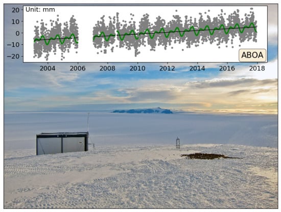
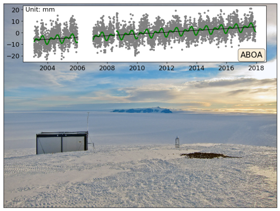
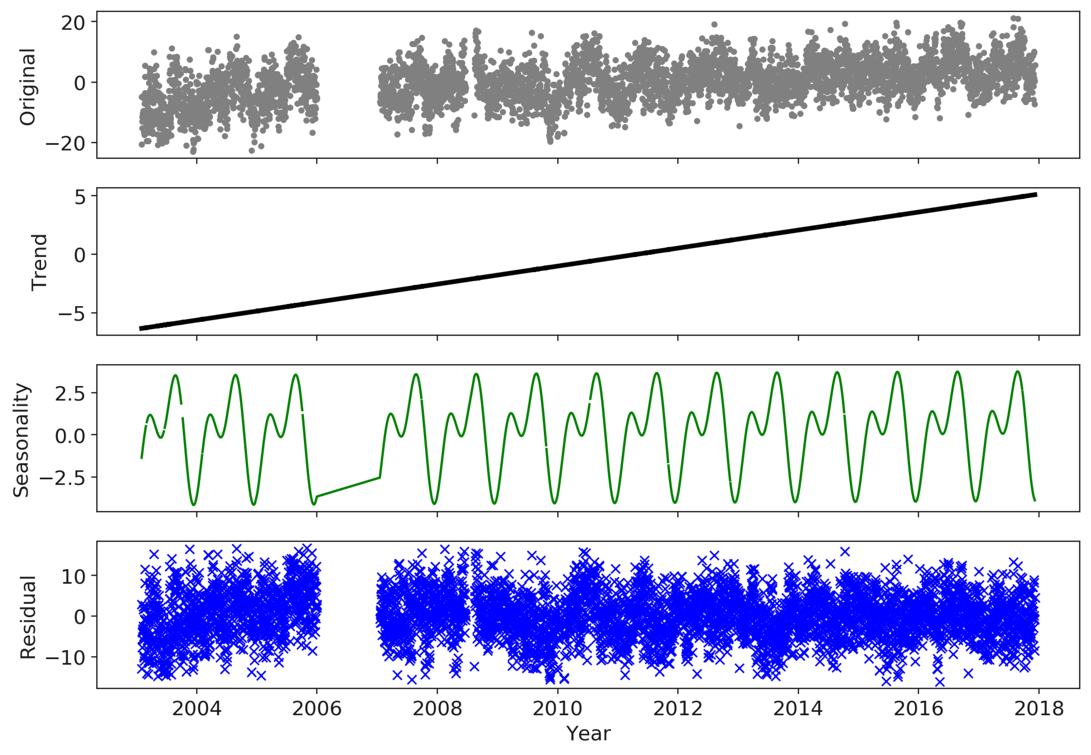
Figure 14 illustrates the movement in the vertical direction and its signal decomposition. The vertical movement consists of a linear trend and seasonal signals. The trend was found to be upwards at a rate of 0.79 ± 0.35 mm/year. The seasonal signals include annual and semiannual components. The amplitude of the annual signal was estimated to be 2.43 ± 0.57 mm, whereas the amplitude of the semiannual signal was estimated to be 2.14 ± 0.42 mm. The maximum amplitude is reached on 23/24 August while the minimum in 13 December. However, these seasonal signals are modelled under the assumption of constant yearly amplitude. Whereas such assumption allows to determine a significant part of the variation, it does not capture the inter-annual variations.
3.3. Environmental Loading
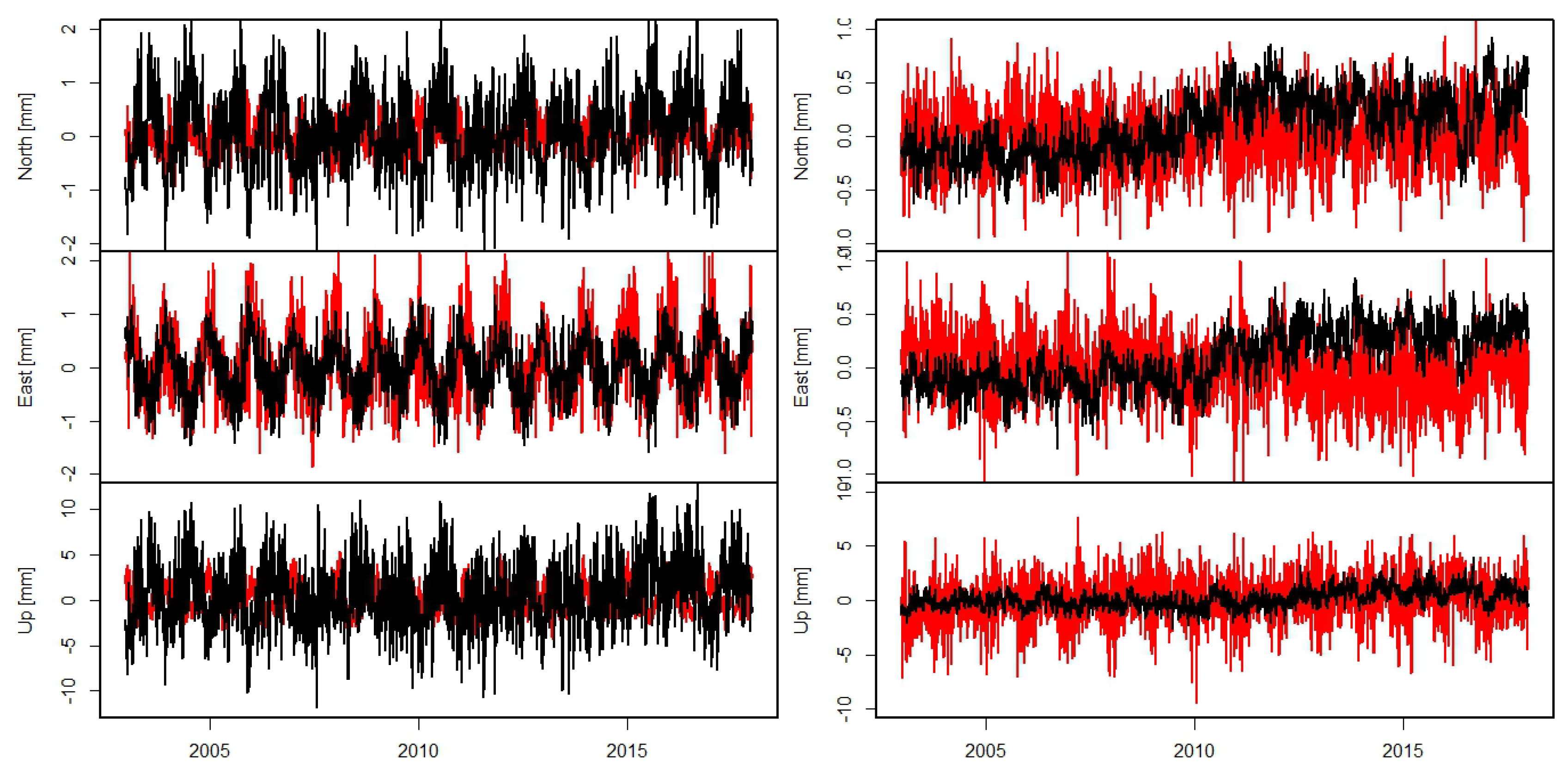
The four time series that were used are depicted in
Figure 15. The black curves are computed by the EOST. Their atmospheric loading is computed using the ECMWF operational model with 3 h resolution, averaged to daily values. The non-tidal loading is from the ECCO2 ocean bottom pressure model [
72], which provides daily values. The red curves were interpolated from the GFZ loading grid using bilinear interpolation. The atmospheric loading is computed from the same 3 h ECMWF operational model, but for the non-tidal ocean loading the MPIOM model [
73] is used with 3 h resolution. The atmospheric loading shows a variability of few millimetres in the horizontal components and a few centimetres in the vertical. The non-tidal ocean shows a smaller variation both in vertical and horizontal.
We studied the effect of the environmental loading on the time series rms and trends. We did the time series analysis before and after removing the atmospheric and non-tidal ocean loading. The effect was unremarkable, as removing the loading affected the trend below the 0.01 mm level and increased the residual rms in all three components. For example, using the EOST products, the trend of the up-component decreased from 0.79 to 0.74 mm/year and the uncertainty for the trend increased from 0.35 to 0.48 mm/year. The residual rms increased from 5.7 to 6.1 mm.

 ,
, 


