1. Introduction
Forest fires are disastrous natural hazards that are sudden, strong, destructive, and difficult to handle, causing damage and loss to ecological ecosystems and human beings [
1,
2,
3,
4]. In addition, the biomass burning that is caused by forest fires is a vital factor for landcover change as well as climate change, and is a significant source of both aerosols and atmospheric trace gases [
5,
6,
7,
8]. Consequently, there is an urgent need to mitigate the impact caused by this global and recurring phenomenon, and because satellite data has the advantage of wide coverage, timeliness, and low cost, it has been pivotal to meet this requirement for more than four decades [
9,
10,
11]. Using these ideal sensors and platforms, researchers have carried out research on fire risk assessment [
12,
13,
14,
15], fuel management [
16,
17,
18], forest fire detection [
19,
20,
21,
22,
23,
24], fire behavior modeling [
25,
26,
27], smoke emissions estimation [
28,
29,
30], and analysis of fire impacts on air quality and FRP (fire radiative power) [
31,
32,
33,
34]. In addition, forest fire detection has always been a hot spot of research. By exploiting the fact that the middle infrared (MIR) and longwave infrared (LWIR) spectral channels have great disparities in sensitivity to sub-pixel fire events, scientists have developed many algorithms and products for fire monitoring and detection over the past three decades, based on satellite sensors in geostationary Earth Observation (EO) satellites and Polar-orbiting systems [
10,
35,
36,
37]. Furthermore, these two sensor platforms have inherent differences: EO satellites have high temporal resolution but low spatial resolution, and, in contrast, Polar-orbiting systems have high spatial resolution but low temporal resolution [
11,
38,
39]. Therefore, the existing forest fire detection algorithms that are based on just one of these two systems merely focus on temporal or spatial information independently. Only rare research has considered the spatial and temporal characteristics of satellite data simultaneously when detecting forest fires, although combining the advantages of spatial-based and temporal-based algorithms would make fire detection more accurate and robust [
10,
37,
40,
41,
42].
Spatial-based fire detection algorithms take advantage of the fine spatial resolution of sensors onboard Polar-orbiting platforms, which are commonly classed either “fixed-threshold” or “contextual” algorithms [
43]. Fixed-threshold algorithms identify a pixel containing actively burning fire if the brightness temperature (BT) or radiance in one or more spectral bands exceed pre-specified thresholds [
44,
45,
46,
47]. The optimal threshold value is difficult to determine because of the variability of the natural background in the time and spatial domains, and it is conservatively selected according to the previous historical data [
40,
41,
48]. As a result, many fires will be neglected, especially small fires. When compared with the fixed-threshold algorithms, contextual algorithms are more sophisticated in confirming a true fire pixel [
20,
49,
50]. Firstly, contextual tests typically flag a candidate pixel with a similar series of fixed thresholds. The tests then confirm that the pixel is a “true fire pixel” by exploiting the strong BT contrast between the hot candidate pixel and its cold background, which is calculated by spatial statistics (e.g., average value and standard deviation) within self-adapting size windows around the candidate fire pixel [
21,
48,
49,
51]. If the contrast is sufficiently higher than the pre-specified thresholds, the pixel is identified as a fire pixel [
22]. This method is based upon the premise that the background BT of the candidate fire pixel, which essentially represents the BT of the target pixel in the absence of the fire, can be accurately estimated [
52]. The ambient background pixels are cloud-free and fire-free pixels but, when the sampled areas around the center pixel are severely affected by cloud, it is difficult to obtain enough valid pixels [
22,
53]. In addition, the background reference pixels are assumed to have the same characteristics as the candidate fire pixel in the absence of fire in the contextual test [
37]. Nevertheless, the sampling area around the target pixel has little correspondence to the emission and reflection characteristics of the central pixel, due to factors such as landcover, elevation, relief and weather effect, or PSF (Point Spread Function) effects (i.e., radiance from the fire pixel affecting the signal of the surrounding pixels) [
37,
49,
54]. As a result, these factors cause different sensor responses between the target and background pixels, ultimately leading to inconsistency in their emissive and reflective properties [
40]. Moreover, spatial autocorrelation issues that are caused by undetected cloud and smoke pixels also exist in calculating the background BT, and this will result in the predicted background BT being lower than it actually is [
52]. Furthermore, these issues are exacerbated because the contextual algorithms have high sensitivity to the accuracy of the background BT. Regarding small fires, if the background BT has an error of 1 K, then the fire area could easily be wrong by a factor of 100 or more [
55,
56]. Of note is that machine learning algorithms show bright prospects in object detection [
57,
58,
59], using techniques such as the support vector machine (SVM), Otsu method, k-nearest-neighbor (KNN), conditional random field (CRF), sparse representation-based classification (SRC), and artificial neural network (ANN). Applied to fire detection, machine learning algorithms classify the target pixel into a fire or background binary object by using image classification approaches, which are more robust and automatic than contextual testing [
60]. For this reason, we use the Otsu method to exploit the spatial contextual information, which selects the optimal threshold to distinguish fire by maximizing variance between classes. However, this Otsu algorithm also requires the accurate prediction of background BT and it suffers from the inaccurate estimation of problems mentioned above. These issues hinder the wide application of spatial-based fire detection algorithms and have led to the investigation of temporal-based fire detection algorithms for accurately estimating the background BT.
Temporal-based fire detection algorithms utilize the high temporal frequency data offered from geostationary orbital sensors and detect the fire by analyzing multi-temporal changes of BT [
37,
42,
61]. These algorithms first leverage recent historical time series data to predict the true background BT. Subsequently, if the observed value is sufficiently higher than the predicted background BT in the MIR band, the pixel is identified as a fire pixel. Using temporal information for fire detection was first introduced by Laneve et al. [
62], who exploited a set of prior observations to build a physical model of the surface BT and then detected fire anomaly by using a change-detection technique in successive images from the Spinning Enhanced Visible and Infrared Imager (SEVIRI). Similarly, Filizzola et al. [
42] applied a multi-temporal change-detection technique called “Robust Satellite Technique” (RST) for timely fire detection and monitoring for SEVIRI. For each target pixel, a temporal mean and standard deviation of BT is calculated and it attempted to discriminate active fire pixels by comparing it to the observed value. However, the intrinsic operational limitations of this method are that weather effects and occlusion hinder the valid identification of fire. In order to interpolate the occlusion or missing value, the DTC model has proven to be an ideal method to solve the problem by providing a diurnal variation of a pixel’s BT. Initial work in modeling the DTC, including the Cosine model [
63] and Reproducing Kernel Hilbert Space (RKHS) model [
64], are both unstable when affected by abnormal factors, such as weather fluctuations. This limitation was later addressed by the robust matching algorithm (RFA) [
65], which introduced the singular value decomposition (SVD) technique and outperformed the previous model. This method was refined by Roberts and Wooster [
37] and Hally et al. [
52], whose refinements showed promise for obtaining more accurate background BT data while also being more robust to anomalous data. It is noteworthy that the work by Roberts and Wooster utilizes the Kalman filter (KF) method as a supplement when the RFA shows poor fitting under abnormal data [
66]. KF is a data processing technique for removing noise and restoring real data, which is widely used in optimal state estimation [
67]. Vanden Bergh and Frost [
61] and Van den Bergh et al. [
68] proposed both linear and extended KF algorithms for fire detection, and these algorithms have been proved to be superior to previous contextual tests. For this reason, here we adjusted the method that was developed by Roberts and Wooster [
37] to obtain background BT.
Some researchers have developed temporal-based fire detection algorithms using satellite data offered from Polar-orbiting platforms. Koltunov and Ustin [
40] presented a multi-temporal detection method for Moderate Resolution Imaging Spectroradiometer (MODIS) thermal anomaly detection by using a non-linear Dynamic Detection Model (DDM) to estimate the background BT for discriminating active fire pixels. Similarly, Lin et al. [
41] proposed a Spatio-Temporal Model (STM) for forest fire detection using HJ-1B infrared camera sensor (IRS) images, in this method, a strong correlation between an inspected pixel and its spatial neighborhood over time was employed to predict the background intensity, and then an equivalent contextual test was conducted for fire detection. Lin et al. [
10] developed an active fire detection algorithm based on FengYun-3C Visible and Infra-Red Radiometer (VIRR). This algorithm detects the changes between the predicted MIR value and the stable MIR value of the target area, and the predicted MIR value was calculated by constructing time series data. Although these methods provided good results on the test areas, the quantity and the quality of the training data for predicting the background BT will be a significant impediment for the thermal anomaly detection. This issue will be exacerbated by the sparse data offered from restricted overpass frequency of Polar-orbiting systems, especially when the observed pixel is contaminated by cloud and smoke, and this unavailability of data will reduce the robustness of this method. Therefore, we seek to utilize the high frequency and consistent data provided by EO platforms to mitigate this effect.
The trade-off with EO sensors is that their coarse spatial resolution results in the failure to detect small fires and precisely locate hotspots [
37]. Despite this, the geostationary attitude provides quasi-continuous monitoring and assures very stable observational conditions, which can offset the vulnerabilities in errors of omission that are caused by limited observations using low Earth orbit (LEO) data, especially when the fire activity is obscured by cloud and smoke during the period of sensor overpass [
52]. These superior revisit time characteristics are crucial for detecting short-living fires, starting fires, and fires with a strong diurnal cycle [
42]. In addition, this long-term dataset with very high repeat cycles could provide timely and early fire information, which can assist both fire authorities and the general public to mitigate the impact of wildfires. Moreover, the datasets offered from new sensors, such as the Japanese Meteorological Agency’s Advanced Himawai Imager (AHI) and the NOAA’s Advanced Baseline Imager (ABI), have unprecedented spatial, radiometric, and temporal resolutions. These “state-of-the-art” datasets will mitigate the bad effects of the aforementioned issues in active fire detection to some extent.
Although these temporal-based fire detection algorithms performed well in studied areas, they seldom take advantage of the spatial contextual information. They have only exploited the temporal information to predict background BT in MIR channel for a single pixel, and they confirm the fire through judging whether the observed BT positively deviates enough from the normal background BT at the pixel level. These deviations among different pixels in a suitable window can provide a variety of spatial contextual information for the target pixel, and thus they are very important for active fire detection. This information is fully exploited in spatial-based fire algorithms but it is often ignored in temporal-based fire detection algorithms. This limitation has been mentioned by many researchers [
10,
37,
40,
41,
42]. Hence, there is a need to merge the independent temporal and contextual information to improve the performance of fire detection algorithms.
Here, we present a novel spatiotemporal contextual model (STCM) that fully exploits the Himawari-8 satellite data’s temporal and spatial contextual information, and merges them to detect active forest fire. The STCM relies on the accurate background BT prediction by using the KF and improved robust fitting algorithm (IRFA). In addition, to achieve a more robust fire detection method, the proposed model adds spatial information to the anomaly detection by using the Otsu method and introduces a temporal test to correct the fire detection results. A total of four fires occurred in East Asia and Australia in 2016 were used to validate the STCM method. We examine the performance of this STCM algorithm against results from the MODIS MOD14/MYD14 active fire products and compare STCM results with those of the contextual and temporal algorithms.
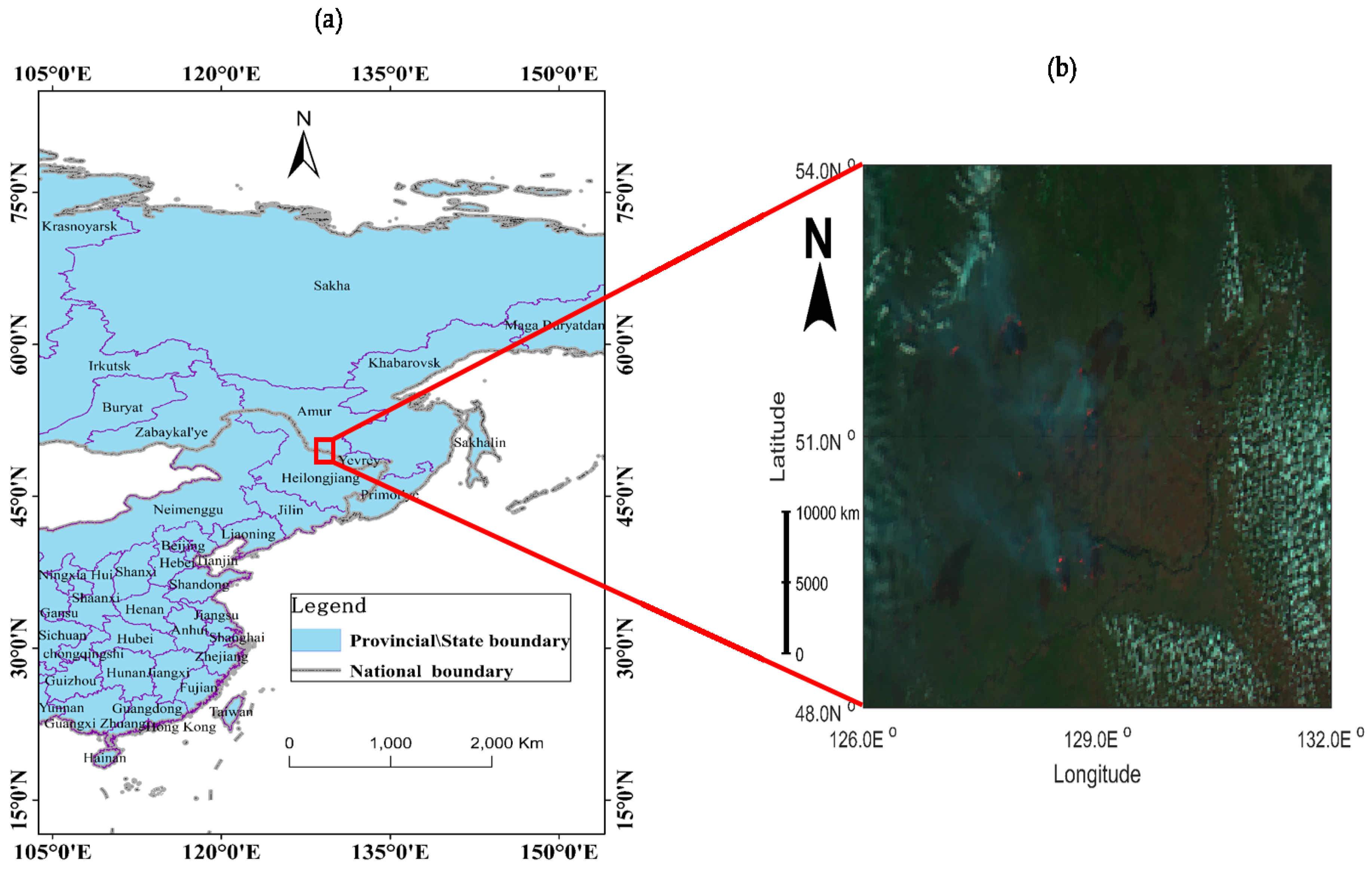
2.1. Case Study Fires
Four fires in 2016 were chosen for the preliminary evaluation of the STCM algorithm. These fire located in Bilahe of northeastern China [
69], on the border between China and Russia [
70], and in Adelaide [
71] and Tasmania [
72] in southern Australia. The detailed information is shown in
Table 1, and cross-border denotes the fire that occurred on the border of China and Russia. The selected year was dominated by extreme weather, with a high number of fires occurring worldwide due to reduced fuel moisture and humidity. As an example shows in
Figure 1, the selected region is a typical boreal forest, where fire is widespread and is the region’s most dynamic disturbance factor. This boreal forest fire in this year was the largest and most damaging in recent history, especially in the Amur region where three major fires covered more than 500,000 hectares [
73]. The low prevalence of cloud cover in ROIs (region of interest) during the selected time, allows for an ideal test-bed for the proposed model to detect forest fires.
2.2. Himawari-8 Satellite Data
This work uses images from the Himawari-8/AHI (140.7°E, 0.0°N), a new generation of Japanese geostationary meteorological satellite, which was successfully launched on 17 October 2014. AHI-8 has significantly higher radiometric, spectral, and spatial resolution as compared to its geostationary predecessor MTSAT-2. It has temporal and spatial resolutions of 10 min and 0.5–2.0 km, respectively [
74]. In addition, imagery is available covering an entire earth hemisphere across East Asia and Australia. The standard product that was used in this model is the available Himawari L1 full disk data (Himawari L1 Gridded Data), which consists of solar zenith angle (SOZ), satellite azimuth angle, solar zenith angle, solar azimuth angle albedo (reflectance*cos (SOZ) of band01~band06, BT of band 07~band 16, along with observation hours (UT). The detailed information is available on website
https://www.eorc.jaxa.jp/ptree/userguide.html, and the standard product was downloaded via FTP (File Transfer Protocol) in NetCDF (Network Common Data Form) format. The bands that were selected for this study are shown in
Table 2. The main bands selected for fire anomaly detection are the MWIR band (band 7, 3.9 μm) and LWIR band (band 14, 11.2 μm), corresponding to 4 μm and 11 μm bands of MODIS, which are the most important bands used for fire detection. We obtain images of the period of the fire and one-month time before the fire. The total number of images used for the analysis was 163 × 142. The improved algorithm is implemented using MATLAB on a supercomputing platform.
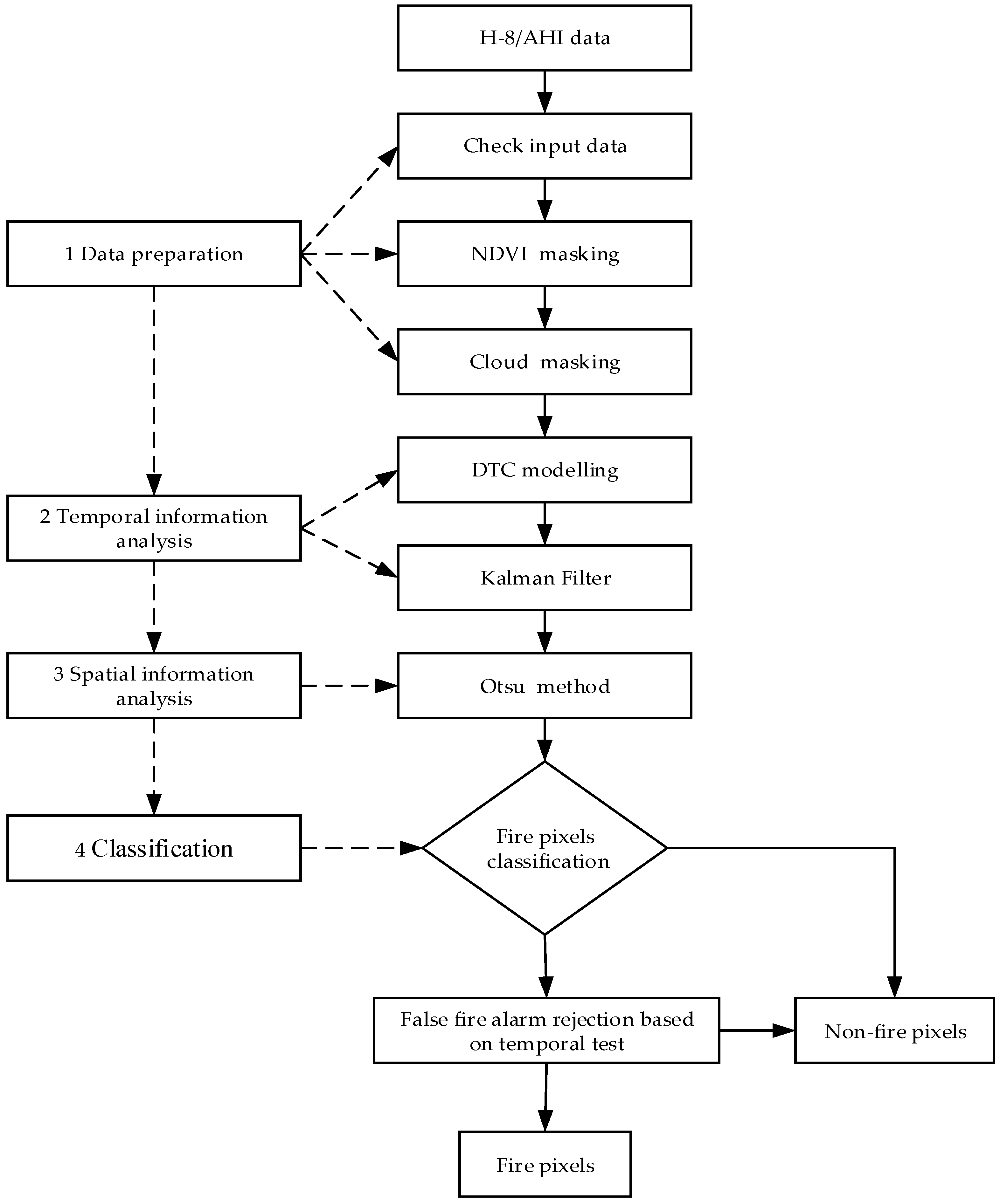
2.3. Overview of the Improved Algorithm
The new algorithm was implemented using a four-step process: data preparation, temporal information analysis, spatial information analysis, and classification. An STCM method workflow is illustrated in
Figure 2. The first step is data preparation to provide the data under normal undisturbed conditions, including check input data, NDVI (Normalized Difference Vegetation Index) masking, and cloud masking. The second step utilizes DTC modelling and KF to predict the true background BT of band 7 and band 14. Once the true background BT has been obtained, the spatial deviation between the observed value and predicted background BT is used in the third step to detect the fire while using the Otsu method [
75]. The final step is to identify pixels as true fire pixels by using a temporal test to correct the fire detection result.
2.4. Data Preparation
2.4.1. Cloud Masking
Cloud coverage is a major inhibiting factor in any satellite fire detection setup and an appropriate cloud mask is critical for accurate active fire detection [
53]. Clouds often cause the pixel BT to be low and to make the reflectance or albedo high in the visible and near-infrared bands. This study utilizes a criterion given by Xu et al. [
76] to remove the cloud-covered pixels from AHI images, which includes a series of spatial and spectral differencing tests.
2.4.2. Forest Fuel Mask Model
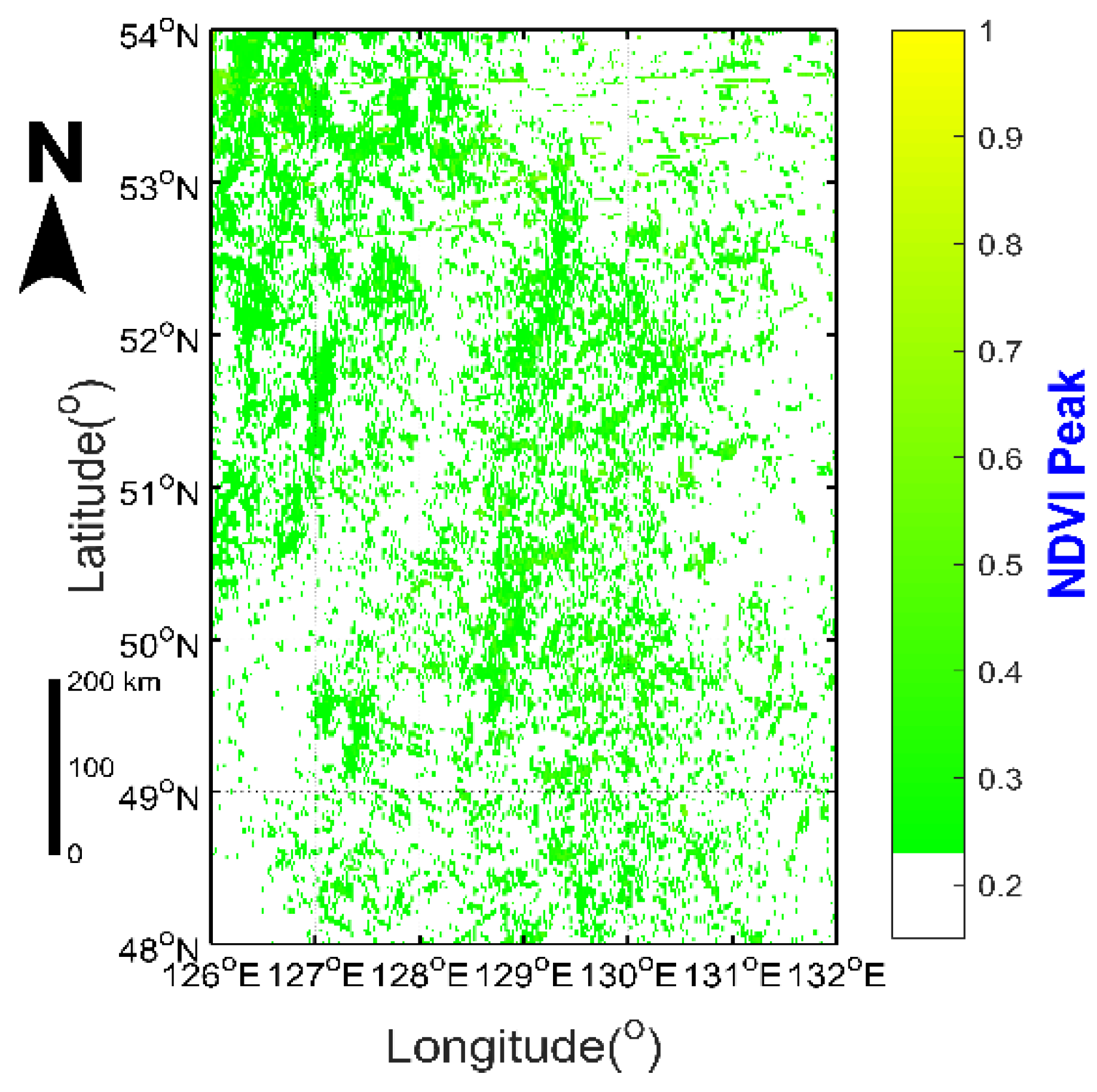
NDVI (normalized difference vegetation index) is calculated by visible and near-infrared channels, as shown in Equation (1), and can reflect the vegetation phytomass. The NDVI mask in fire detection is based on the assumption that only pixels with NDVI value exceeding the default threshold would be considered to have enough fuel to maintain a fire [
77]. This masking should eliminate most of the false alarms that are caused by non-vegetation surfaces, such as bare soil, rocks, water, and urban area. A fuel mask is shown as Equation (2), which uses the peak of NDVI in one month of continuous cloud-free images before the fire event (
Figure 3).
Here, and are the reflectance in band 3 and band 4, respectively. The pixels that satisfy Equation (2) form a mask signifying the valid pixels for the fire detection.
2.5. Temporal Information Analysis
2.5.1. Modelling the Diurnal Temperature Cycle (DTC)
The DTC curve fitting method that is presented here is adapted from the robust fitting algorithm (RFA) work done by Roberts and Wooster [
37], which was originally described by Black and Jepson [
65] and uses a singular value decomposition (SVD) method to reduce the influence of outliers by interpolating the missing data. This method extracts 10 anomaly-free DTCs in one target month period when the fire occurred as a training dataset for use in an SVD. The DTC must have less than six cloud- or fire-affected observations in every 96 images to be selected as an anomaly-free DTC. If a pixel has less than ten anomaly-free DTCs, then a database of contamination-free DTCs of all other pixels will fill in the training dataset for the SVD process. Hally et al. [
66] indicated that using these supplemental DTCs to populate an SVD leads to training data fragility and could introduce errors in the subsequent fitting process.
Therefore, we make two improvements in this RFA, and this modified algorithm is called the improved robust fitting algorithm (IRFA). Firstly, the period in which to select contamination-free DTCs for the training dataset is the month before the fire broke out instead of the time when the event occurred. This adjustment is based upon the premise that the two consecutive months have the similar DTC variations in the absence of fire, and will obtain more contamination-free DTCs in theory to mitigate the negative impact that is caused by insufficient input in DTC samples, which will improve the training data availability. Secondly, for every pixel, the training dataset is not DTCs with a limit of fixed anomaly affected observations in a month but rather 10 minimum anomaly-impacted DTCs. This refinement will completely remove the error that is introduced by the process that uses supplemental DTCs to populate an SVD. Although these two improvements will eliminate the error mentioned by Hally et al. [
66], the number of outliers of DTCs that are selected for the training dataset may exceed six, and that could weaken the stability of the model. However, data offered from the high frequency of AHI provides 142 images every day, which greatly exceeds the SEVIRI data utilized by Roberts and Wooster [
37], which was only 96 images per day. This high-performance satellite data will compensate for the aforementioned issues to a large extent.
Cloud-affected observations were identified using the cloud detection algorithm used in a study of AHI fire detection by Xu et al. [
76]. Observations were removed due to the strong difference between observed MIR and LWIR channel values when the fire occurs [
10]. The following inequalities are the criteria for extracting fire affected pixels:
Here,
and
are BT in band 7 and band 14 of the AHI image, and
is the difference between them. In daytime, fire-affected pixels were identified where
is limited to 30 K in Equation (3), and 15 K at night in Equation (4).
and
are albedo in band 3 and band 4, pixels were identified at night in Equation (6) by the low albedo of visible bands (0.64 μm and 0.86 μm), and the other time periods are all daytime in Equation (5) [
78].
The SVD method that was used reduces dimensionality and keeps useful information while maintaining a low error level. For each pixel, a training data matrix
was constructed based on 10 minimum anomaly-impacted DTCs in one month. An SVD decomposes the training data matrix
into a number of orthogonal vectors
which represents the principal component directions of the training data, along with the diagonal matrix
, which contains sorted decreasing singular values along the diagonal, and the matrix
which contains coefficients for the reconstruction of each column of
in terms of the principal component directions, as shown in Equation (7):
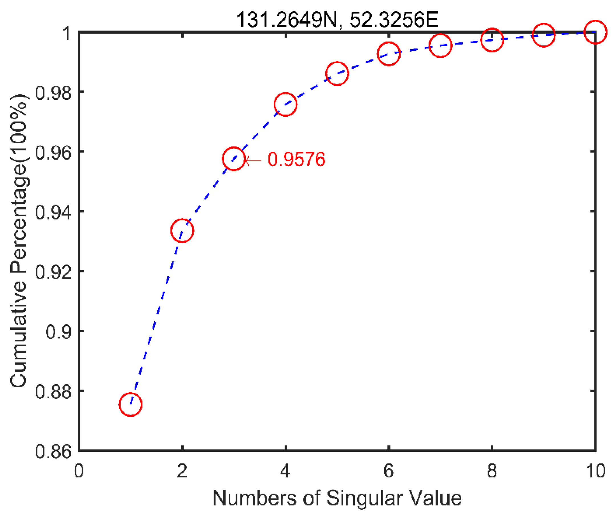
To exploit the most salient information of component vectors while minimizing the effect of overfitting caused by these extra degrees of freedom in the component vectors, the cumulative percentage of singular values should at least 95% [
79], As an example shows in
Figure 4, as the number of singular values along the diagonal increases, and
contributes little to the DTC fitting process. For any input observation DTC
of a pixel, a new vector
can be approximated by reconstructing the principal components in Equation (8):
where
is a series of scalar valued calculated by taking the dot product of the input DTC
and the principal component
.
essentially describes the number of basis vectors used to reconstruct the fitted estimate of the DTC
.
At this point, to minimize the effects of outliers on the robust determination of the entire DTC and robustly estimate the coefficients
, the quadratic error norm is used in Equation (9), because it has more sensitivity to outliers than the least-squares method:
Here,
is the residual between the estimated DTC
and input DTC
at time
, and
is a scale factor, which begins with a high value, and it is reduced iteratively when using the gradient steepest descent scheme to minimize the error function and calculate the coefficients
. To reject the effect of instability that is caused by numerous outliers during the error minimization, an outlier mask
is introduced in Equation (10):
The error function is minimized through
, as shown in Equation (11):
The estimated DTC is robust to outliers, such as the observation noise that is caused by atmospheric effects, but the ideal DTC fails to perform sufficiently well in situations where persistent cloud or fires are at the location of interest, or there is missing data [
37]. This problem can be mitigated by employing a linear Kalman filter approach.
2.5.2. Kalman Filter
The Kalman filter (KF) is a data processing technique that removes noise and restores real data [
67]. The standard KF is recursive and it takes into account all previous observations blended with model-based predictions to provide optimal estimates about future states of a system. This indicates that KF can be used to predict the expected background BT of band 7 and band 14. KF is used in the current paper to more accurately fit the DTC model when the IFRA performs poorly in situations where outliers exist. KF estimates the best approximation between the estimated and the true value by combining previous estimates and the new observations. Our KF is implemented using a three-step process: state process, measurement process, and update process.
The prediction of the state variable of DTC is given as:
where
is the state estimate of the system (BT) at step
, and
is the process noise.
is the state transition coefficient and derived from the modeled DTC in the following way:
where
is the modeled DTC estimate. The measurement process of the KF is realized by the linear relationship:
where
represents the observation at time
,
is the a posteriori state estimate, and
is the measurement noise. The two independent noise sources are assumed to obey normal distribution:
where
and
are the process noise and measurement noise variance, respectively, at time
. The process noise
represents the influence of outliers on the ability to model the DTC and it is given in Equation (9). The measurement noise
describes the difference between the measurement and true value, given by:
The update process for the KF will not be repeated here, details can be found in [
37]. Note that the system will assimilate the previous abnormal data into the next prediction when KF adaptively updates, which could weaken the system detection capability for predicting the true background BT and ultimately cause a false alarm [
52,
68]. To solve this problem, we can set the Kalman gain to zero when cloud-contaminated or fire-contaminated observations are propagated during the update process.
2.6. Spatial Inforamtion Analysis
Otsu Method
The Otsu method is a nonparametric and unsupervised method of automatic threshold selection for extracting objects from their background [
75]. This threshold enables the between class variance maximum, and the maximum is very sensitive to change and it can be used for fire detection. This method is more robust, sensitive, and automatic than the contextual testing and temporal detection, even in detecting small fires [
60]. Here, we use it to better detect the fire by exploiting the fact that the MIR and LWIR spectral channels have great disparities in sensitive to sub-pixel high BT events [
37]. The Otsu method is useful, because fire events cause a steep rise in maximum between class variance in a reasonable pixel window, and this rapid change can be used as an important parameter in active fire detection. At this point, assume that an image has
flag values, and the flag values are differences between the observed value and the modeled BT in MIR (band 7) (
), and the difference of difference between the observed value and the modelled BT in MIR (band 7) and LWIR (band 14) (
). Subsequently, the pixels of the image are divided into groups as follows: background objects deemed to be pixels containing no fire have flag values from 0 to
, and target objects are fire-affected pixels having flag values from
to
. To maximize the between class variance, we need to perform the following steps:
Step 1: Flag value probability distribution for both the groups is calculated as:
where
is the probability of each flag value, which is calculated by the numbers of pixels having
flag value
and the total number of pixels is
.
Step 2: Means for background and target groups are calculated as:
Step 3: Total mean for both the groups is denoted by
Step 4: Between class variance is
The purpose of the Otsu method is to choose the optimal threshold to maximize the between class variance. Thus, the objective function is
2.7. Fire Detection Algorithm
The purpose of this section is to detect fire pixels by exploiting the spatial and temporal characteristics of H-8 data. We use maximum between class variance and BT of the MIR band as the main parameter in fire detection, which is sensitive to BT changes. The fire detection algorithm can be realized as four processes: cloud and NDVI masking, potential fire pixel judgment, absolute fire pixel judgment, and relative fire pixel judgment that is based on STCM.
A pixel is classified as a potential fire pixel if it meets the following conditions before cloud and NDVI masking.
where
and
are the differences between the observed value and the modelled BT in band 7 and band 14, an
is the observed BT in band 7.
For absolute fire detection, the algorithm requires that at least one of two conditions be satisfied. These are:
For realative fire detection, the algorithm requires that at least one of two conditions be satisfied. These are:
For calculating the maximum between the class value of flag values, the valid background pixels surrounding the potential fire pixel are defined as those that (1) meet the NDVI mask test in Equation (2), (2) are cloud-free, and (3) are fire-free background pixels. Fire-free background pixels are in turn defined as those pixels for which
(
at night) and
(
at night). To maximize the use of BT variation characteristics and reduce other errors that are caused by an excessive window [
53], the background window size is initially set to
, but it is allowed to grow up to
until the number of valid pixels is at least three and the proportion in the window is at least 25%. If these conditions cannot be satisfied, then the algorithm flags the pixel as a non-fire pixel.
Finally, a temporal test is used to correct the fire detection result. The specific algorithms are:
Here,
,
,
, and
are the detection results in five continuous timeslots. The temporal test is based on the idea that fires occurring within 20 min with LEO fire product are classified as synchronous instances [
52], which indicates all AHI anomalies during this period are treated as a single fire observation. In Equation (28), if a pixel were deemed to contain the fire but the last and next timeslots were identified as having no fire, then the detection result will be regarded as a false alarm. Similarly, in Equation (29), if a pixel were deemed to contain no fire, but the last and next timeslots were identified as having fire, then the pixel will be regarded as a fire point at time
.
4. Discussion
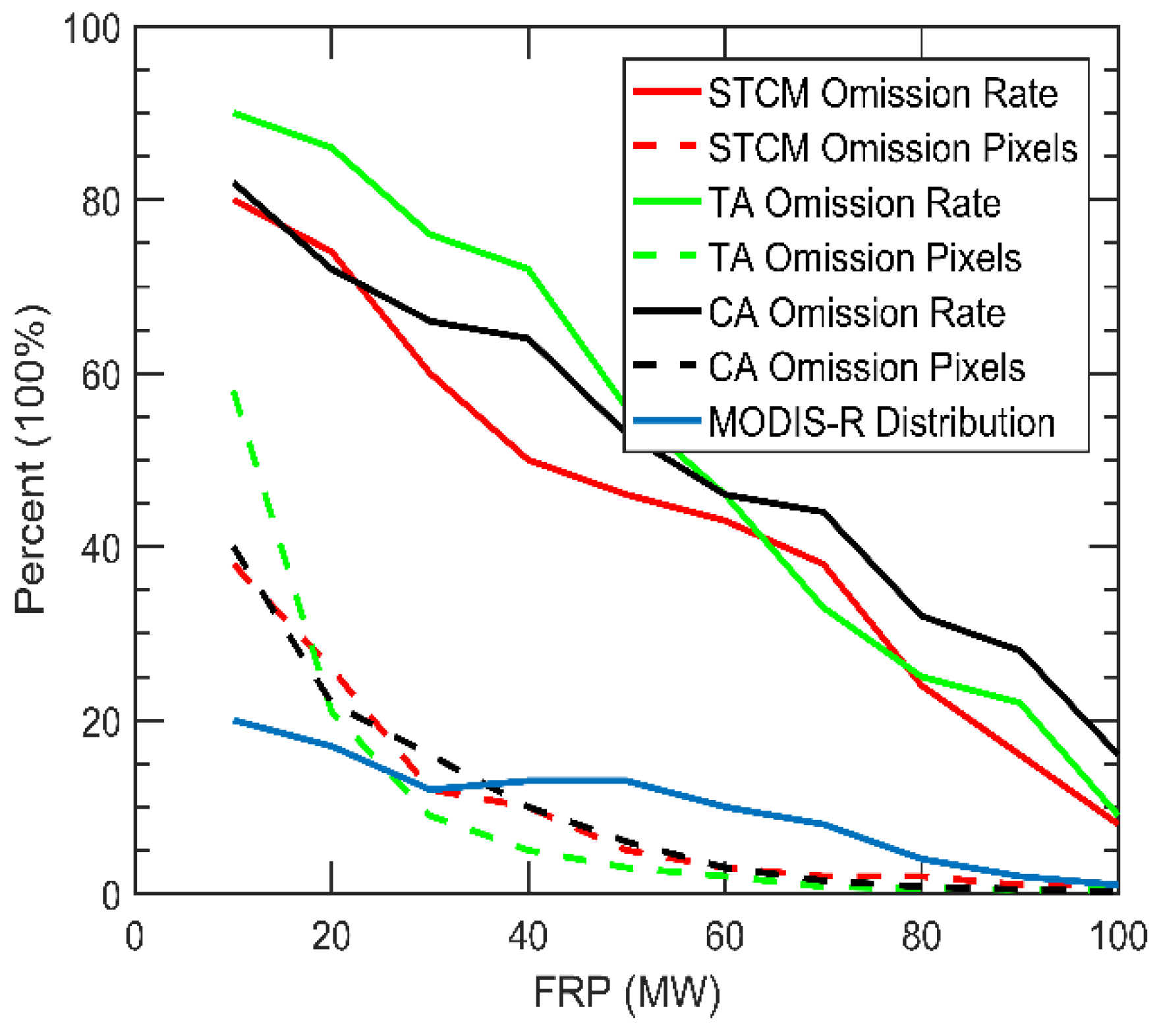
Our results indicate that the new forest fire detection method based on STCM obtains higher detection accuracy than the traditional contextual algorithm and spatial algorithm. Moreover, the advantage of using STCM for forest fire detection based on AHI data includes fully exploiting and merging the temporal and spatial contextual information of band 7 and band 14. The temporal information was used to obtain the DTC variation of the true background BT for each pixel, based on the IRFA. Our findings suggest the IFRA is more robust and accurate than the contextual method and RFA, especially during periods with many outliers. When compared with the RFA, the IRFA advantage is mainly attributed to the training data being derived from the month before a fire occurs rather than the month during which the fire occurs. This change will greatly reduce the positive anomalies caused by fire. In addition, the composition of the training dataset does not require DTCs with a limited number of fixed anomaly-affected observations in a month, but rather uses the ten minimum anomaly-impacted DTCs. This refinement will completely remove the error that is introduced by the process of using supplemental DTCs to populate an SVD. When compared with the contextual method, the advantage of this IRFA is that it utilizes SVD and KF, dual approaches in curve fitting, which is effective in removing the abnormal data and keeping the model stable. To exploiting spatial information, the Otsu method was introduced to detect fire, which is more robust, sensitive, and automatic than the contextual algorithm and temporal algorithm, even for the detection of small fires. This advantage is confirmed in the
Figure 6 and
Table 5, whose results imply that STCM performs best in overall omission rate and commission rate, especially in low FRP fires (<30 MW). In addition, our results infer that the temporal correction brings a significant improvement in STCM accuracy with a marked decrease both in commission error and omission error. This demonstrates that the continuous real-time observations are highly effective to improve fire detection capability, and also illustrates that the high temporal satellite data can be utilized for the dynamic fire monitoring, which was also shown in [
51] via research that took advantage of repeated visits of AHI to determine the fire ignition times.
Although the STCM has shown impressive performance for fire detection in this study, lacking the accurate, verified cloud mask product would be the biggest obstacle to the implementation of the algorithm. As noted in [
81], because of the relatively young age of the AHI sensor, there are no standard cloud mask algorithms for fire detection. There are ongoing issues that the cloud edges and thin cirrus are often not identified by a cloud scheme but still influence the raw BT. These omitted effects would influence the fitting degree of the true background BT, and ultimately cause the fire detection result to contain a high commission error rate. Therefore, cloud mask accuracy improvement that is based on AHI data should be a priority.
The accuracy of STCM is based upon an important premise that the ideal DTC in the absence of the fire is predicted accurately. The accuracy of the model DTC relies on a couple of factors. Firstly, the quality of the training data used for the IFRA is affected by the number of fire-affected or cloud-affected values during the selected month. This shows a requirement for the cloud- and fire-affected product. The cloud mask product has been discussed above, and, as for the fire-affected product, similar to [
10], a rudimentary threshold was used to reject the fire-affected observations. However, a more appropriate approach may apply an existing temporal/contextual fire product to identify the fire pixels, as shown in [
37], which use a contextual fire product for fire pixel detection. Unfortunately, there is no such mature fire product for the AHI. This problem may be solved by [
53], which uses a contextual method to estimate the background BT based on AHI. If the anomalies are relatively high, we may move time forward to select the training data by carefully considering the month variation of the background BT. In addition, the higher temporal AHI data allow for more anomalies than the SEVIRI data with a 30-min sampling frequency used in the robust fitting technique. Secondly, the robustness of the selected method to estimate the ideal DTC is affected by the number of outliers; as the number of the anomalies increase, the curve is poorly fitted, as shown in
Figure 5c,f. This illustrates the limitation of using the IFRA with greater degrees of freedom. In this situation, the true BT may be replaced with the temporal mean BT, similar to what is done in [
42], which applied a “Robust Satellite Technique” (RST) to SEVIRI to detect fire. Finally, the raw BT was influenced by other undetected occlusions, for example, smoke, fog, or even maybe a huge canopy.
Considering setting the appropriate threshold for the contextual test when using the Otsu method, the Otsu method performed reasonably well for fire detection in comparison to the traditional temporal fixed threshold and contextual algorithms. This advantage is mainly because the Otsu method can detect slight signal variations. Moreover, the parameters that were adopted relate to great disparities in sensitivity to fire events in the MIR and LWIR spectral channels; good parameter choices will magnify these signal variations. Of note is that the diurnal variation of this signal could be used for a fire danger rating by setting an appropriate threshold range, which will assist in fire risk management. In addition, this dynamic diurnal variation curve will contribute to the threshold selection for fire detection. This is similar to the temporal correction, which corrects the detection result by a dynamic continuous observation to calculate the number of single fires that were detected in a fixed temporal window. The approach is mainly used to reject false alarms by the occasional factors or prevent true fire pixels from being omitted, especially the fire omitted because of low intensity during the initial stage or end phrase despite a fire being present. There is an ongoing issue of how to set an appropriate temporal window; an optimal choice may relate to the combustion characteristics of forest fuels in the study area.
The accuracy of STCM for fire detection in this study is quite good, but the lack of validated standard fire products that are based on temporal/contextual algorithms from the sensor data remains an issue for the accurate performance comparison of these three fire detection algorithms. In the temporal algorithm, a high threshold of 5 K was set to generate the fire product to reduce the high rate of false alarms at the expense of a lower rate of successful anomaly detections. A lower threshold will introduce more false alarm errors; yet, it will have the advantage of more likely detecting small fires. The choice of the threshold can make the temporal model inaccurate, especially because the main omission error caused by missing small fires. The MODIS fire product was used as a reference dataset in this study for the sake of global application, although MODIS often omits small fires with a relatively high BT threshold. Therefore, the small fires that were detected by the three algorithms but omitted by the MODIS will be the main source of the commission errors at the lower FRP. This may indicate that the true accuracy of the three algorithms is higher than it appears. Moreover, the results show the omission error is mainly caused by small fires that AHI misses but MODIS detects, as shown in
Figure 6. Therefore, determining how to distinguish the small fires that are detected by AHI, MODIS, or both should be a priority. This limitation may be broken by introducing other higher spatial fire products or adjusting the MODIS fire algorithm for ROIs.
Overall, the STCM that is described in this paper fully exploits Himawari-8 Satellite data’s temporal and spatial contextual information, merging them to achieve forest fire detection that performed well from an accuracy standpoint. The most intuitive benefit is that in locating the fire point, the AHI spatial resolution is too sparse, so we may synergistically use finer sensors like GaoFen-4 (GF-4) or Unmanned Aerial Vehicles (UAV) in combination with the Himawari-8 satellite data to precisely position the sub-pixel fires. Furthermore, the STCM could provide timely and accurate on-site fire information based on AHI data with a high temporal resolution [
84], which is crucial for emergency responders and the general public to mitigate the damage of the forest fires, especially for some small-sized or starting fires that may develop into a megafire. In addition, timely quantified fire information would provide a more accurate estimation of biomass burning emissions, which is closely linked to calculating the FRP or monitoring air quality. Moreover, as noted in [
23], the finer spectral information of AHI can be utilized for tracking the fire line at 500 m resolution. Future work should combine the spectral, temporal, and contextual information to better exploit the capability of fire detection based on AHI data.
In addition to its application to the Himawari-8 data, STCM could also be used for similar sensors while considering the quality and quantity of the training data carefully. Furthermore, this method could have application in rapidly evolving spatiotemporal events, such as landcover, flooding, earthquake, and thunderstorms [
85,
86,
87,
88]. In addition, taking consideration of the abundant time series data offered from geostationary imagery, we might introduce machining learning techniques, such as CNN (convolutional neural network), to better understand the capabilities of continuous observation. Finally, due to the inherent defects in temporal-spatial traits in synchronous satellites and polar orbit satellites, their synergy would provide a promising blueprint for earth observation.


