Figure 1.
(a) Spatial distribution of about 40,000 Automatic Weather Station (AWS) (red point) and three sub-regions, (b) AWS observed hourly precipitation at 02 UTC 8 June 2015 and (c) time series of correct and dubious AWS numbers from 00 UTC 1 July to 23Z 31 July 2015.
Figure 1.
(a) Spatial distribution of about 40,000 Automatic Weather Station (AWS) (red point) and three sub-regions, (b) AWS observed hourly precipitation at 02 UTC 8 June 2015 and (c) time series of correct and dubious AWS numbers from 00 UTC 1 July to 23Z 31 July 2015.
Figure 2.
Spatial distribution of the 208 hydrological stations (red points). The two blue lines correspond to the annual 800-mm and 400-mm precipitation contours, which are used to divide China into three sub-regions: Reg. I, Reg. II and Reg. III.
Figure 2.
Spatial distribution of the 208 hydrological stations (red points). The two blue lines correspond to the annual 800-mm and 400-mm precipitation contours, which are used to divide China into three sub-regions: Reg. I, Reg. II and Reg. III.
Figure 3.
Scatter plots between the (a) correlation coefficient, (b) bias and (c) root mean square error (RMSE) and the distance from the hydrological station to its nearest benchmark station.
Figure 3.
Scatter plots between the (a) correlation coefficient, (b) bias and (c) root mean square error (RMSE) and the distance from the hydrological station to its nearest benchmark station.
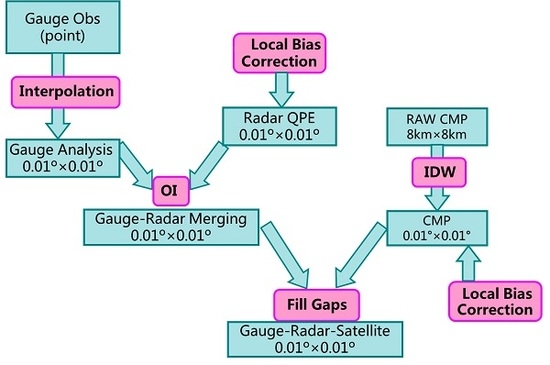
Figure 4.
Flowchart of the hourly gauge-radar-satellite precipitation merging algorithm at the 0.01 degree lat./lon. grid box. In this figure, the term Gauge Obs, ‘CMP’ and ‘QPE‘ mean the gauge precipitation observations, CMORPH satellite precipitation dataset and the quantitative precipitation estimation derived from weather radar.
Figure 5.
Time series of (a) correlation coefficient and (b) RMSE (mm/6 h) of radar (Rrain, red line) and satellite (Srain, black line) precipitation products at the 6-h temporal interval from June–August 2015.
Figure 5.
Time series of (a) correlation coefficient and (b) RMSE (mm/6 h) of radar (Rrain, red line) and satellite (Srain, black line) precipitation products at the 6-h temporal interval from June–August 2015.
Figure 6.
Curves for RMSE and the number of influence gauges with the increasing number of gauges over Reg. I (a), II (b) and III (c), respectively, in China.
Figure 6.
Curves for RMSE and the number of influence gauges with the increasing number of gauges over Reg. I (a), II (b) and III (c), respectively, in China.
Figure 7.
Error variance curves for the hourly radar QPE with precipitation at the 0.01° × 0.01° resolution in the six sub-regions in China. (a) Northeast (east of 110°E, north of 42.5°N), (b) north (east of 110°E, 35°N~42.5°N), (c) Jianghuai (east of 107.5°E, 27.5°N~35°N), (d) south (east of 107.5°E, south of 27.5°N), (e) southwest (97.5°E~107.5°E, south of 35°N) and (f) east of northwest (97.5°E~110°E, north of 35°N) (Shi and Xu, 2006).
Figure 8.
Same as
Figure 7, but for the error correlation coefficient of the radar QPE with the distance between any two points.
Figure 8.
Same as
Figure 7, but for the error correlation coefficient of the radar QPE with the distance between any two points.
Figure 9.
Error variances for the hourly gauge-based precipitation analysis under the different (a) gauge “truth” precipitation and (b) gauge network density at the 0.05° (blue line), 0.10° (red line) and 0.25° (green line) resolution. In this figure, Neg means the number of equivalent gauges.
Figure 9.
Error variances for the hourly gauge-based precipitation analysis under the different (a) gauge “truth” precipitation and (b) gauge network density at the 0.05° (blue line), 0.10° (red line) and 0.25° (green line) resolution. In this figure, Neg means the number of equivalent gauges.
Figure 10.
Simulated error variances changing with the precipitation and the gauge network density at the three grid resolutions of (a) 0.05°, (b) 0.10° and (c) 0.25°.
Figure 10.
Simulated error variances changing with the precipitation and the gauge network density at the three grid resolutions of (a) 0.05°, (b) 0.10° and (c) 0.25°.
Figure 11.
Spatial distribution of bias with and without local bias correction for radar (a,b) and satellite (c,d) at 0.01 degree lat./lon. grid.
Figure 11.
Spatial distribution of bias with and without local bias correction for radar (a,b) and satellite (c,d) at 0.01 degree lat./lon. grid.
Figure 12.
The same as
Figure 11, but for RMSE.
Figure 12.
The same as
Figure 11, but for RMSE.
Figure 13.
The same as
Figure 11, but for correlation coefficient.
Figure 13.
The same as
Figure 11, but for correlation coefficient.
Figure 14.
(a) Time series of correlation coefficients between the hydrological precipitation observations and gauge precipitation analysis (Grain); (b) time series of correlation coefficients between the hydrological precipitation observations and radar QPE (Rrain) and at the three sampling windows, wd0, wd1 and wd2, respectively, from June–August 2015.
Figure 17.
Spatial distribution of the precipitation event occurred at 11Z 8 June 2015 with the resolution of 0.01°depicted by (a) gauge-based precipitation analysis (gauge analysis), (b) radar QPE, (c) Original CMORPH product (Orig_CMPH) and (d) the gauge-radar-satellite merged precipitation product (merged) (unit: mm/h).
Figure 18.
Values of ETS, TS, POD and FAR for gauge analysis, radar QPE, CMORPH and CMPA-1km products at a 6-h temporal resolution in 2015 with different precipitation threshold values.
Figure 18.
Values of ETS, TS, POD and FAR for gauge analysis, radar QPE, CMORPH and CMPA-1km products at a 6-h temporal resolution in 2015 with different precipitation threshold values.
Table 1.
Statistical metrics for daily precipitation between the hydrological station (MWR Precip.) and its nearest benchmark station (Benchmark Precip.) at three time scales.
Table 1.
Statistical metrics for daily precipitation between the hydrological station (MWR Precip.) and its nearest benchmark station (Benchmark Precip.) at three time scales.
| | MWR Precip. (mm/d) | Benchmark Precip. (mm/d) | CC | RMSE (mm/d) | Bias (mm/d) | Sample Number |
|---|
| Annual mean | 3.365 | 3.728 | 0.857 | 5.686 | −0.362 | 74,390 |
Warm Season
(May–September) | 5.092 | 5.469 | 0.839 | 7.803 | −0.376 | 31,249 |
| Cold Season (October–April) | 2.114 | 2.467 | 0.895 | 3.412 | −0.352 | 43,141 |
Table 2.
Contingency table for comparing individual precipitation products () with the hydrological precipitation observations (g). The rainfall thresholds in this paper are 0.1, 1.0, 5.0, 10.0, 20.0, 30.0, 40.0 and 50.0 mm/6 h.
Table 2.
Contingency table for comparing individual precipitation products () with the hydrological precipitation observations (g). The rainfall thresholds in this paper are 0.1, 1.0, 5.0, 10.0, 20.0, 30.0, 40.0 and 50.0 mm/6 h.
| | ≥ Threshold | < Threshold |
|---|
| g ≥ Threshold | Hits (H) | Misses (M) |
| g < Threshold | False alarms (F) | Correct negatives (C) |
Table 3.
Fitting coefficients, a, b and c, at grid resolutions of 0.05°, 0.10° and 0.25°, respectively.
Table 3.
Fitting coefficients, a, b and c, at grid resolutions of 0.05°, 0.10° and 0.25°, respectively.
| | a | b | c |
|---|
| 0.05° | 2.73 | 1.13 | 0.28 |
| 0.10° | 2.43 | 1.08 | 0.17 |
| 0.25° | 1.74 | 1.19 | 0.31 |
Table 4.
Cross-validation results for the radar and satellite estimates with and without the LGC.
Table 4.
Cross-validation results for the radar and satellite estimates with and without the LGC.
| | Radar QPE | CMORPH |
|---|
| Without LGC | With LGC | Without LGC | With LGC |
|---|
| Bias (mm/h) | −0.340 | 0.095 | −0.108 | 0.208 |
| Relative Bias (%) | −18.3 | 5.100 | −5.400 | 10.400 |
| RMSE (mm/h) | 4.447 | 2.219 | 4.931 | 2.798 |
| CC | 0.424 | 0.879 | 0.324 | 0.828 |
Table 5.
Evaluation metrics of individual precipitation observations during the heavy rainfall event that occurred on 8–9 June 2015. NSSL, National Severe Storms Laboratory; MRMS, Multi-Radar/Multi-Sensor.
Table 5.
Evaluation metrics of individual precipitation observations during the heavy rainfall event that occurred on 8–9 June 2015. NSSL, National Severe Storms Laboratory; MRMS, Multi-Radar/Multi-Sensor.
| | CC | RMSE (mm/6 h) | Bias (mm/6 h) | Relative Bias (%) |
|---|
| Gauge Analysis | 0.843 | 2.643 | 0.506 | 44.61 |
| Radar QPE | 0.512 | 3.687 | −0.374 | −32.95 |
| CMORPH | 0.474 | 3.904 | 0.058 | 5.15 |
| CMPA-1km | 0.882 | 2.158 | 0.263 | 23.19 |
| NSSL MRMS (1 km) | 0.855 | 2.1 | --- | --- |
Table 6.
Evaluation metrics of individual precipitation observations in summer and winter seasons at a 6-h temporal resolution. The threshold value is 1.0 mm. ETS, equitable threat score; POD, probability of detection.
Table 6.
Evaluation metrics of individual precipitation observations in summer and winter seasons at a 6-h temporal resolution. The threshold value is 1.0 mm. ETS, equitable threat score; POD, probability of detection.
| | Winter (December–February) | Summer (June–August) |
|---|
| CC | RMSE (mm/6 h) | Bias (mm/6 h) | Relative Bias (%) | CC | RMSE (mm/6 h) | Bias (mm/6 h) | Relative Bias (%) |
|---|
| Gauge Analysis | 0.8705 | 1.1189 | 0.0660 | 12.04 | 0.9418 | 1.7984 | −0.0146 | −1.37 |
| Radar QPE | 0.6789 | 1.7950 | 0.0246 | 4.48 | 0.7416 | 3.8509 | −0.3727 | −35.11 |
| CMORPH | 0.4473 | 1.9252 | −0.3461 | −63.15 | 0.5324 | 5.1322 | 0.1300 | 12.24 |
| CMPA-1km | 0.7998 | 1.4468 | 0.1006 | 18.36 | 0.9257 | 2.0446 | −0.0500 | −4.71 |
| | Winter (December–February) | Summer (June–August) |
| ETS | TS | POD | FAR | ETS | TS | POD | FAR |
| Gauge Analysis | 0.72 | 0.74 | 0.83 | 0.13 | 0.70 | 0.74 | 0.84 | 0.15 |
| Radar QPE | 0.46 | 0.51 | 0.63 | 0.28 | 0.49 | 0.55 | 0.70 | 0.29 |
| CMORPH | 0.27 | 0.30 | 0.33 | 0.20 | 0.35 | 0.41 | 0.61 | 0.44 |
| CMPA-1km | 0.67 | 0.70 | 0.80 | 0.15 | 0.67 | 0.71 | 0.83 | 0.18 |
Table 7.
Evaluation metrics of individual precipitation observations in summer and winter seasons over three sub-regions at a 6-h temporal resolution.
Table 7.
Evaluation metrics of individual precipitation observations in summer and winter seasons over three sub-regions at a 6-h temporal resolution.
| Region I | Winter (December–February) | Summer (June–August) |
|---|
| CC | RMSE | Bias | Relative Bias (%) | CC | RMSE | Bias | Relative Bias (%) |
|---|
| (mm/6 h) | (mm/6 h) | (mm/6 h) | (mm/6 h) |
|---|
| Gauge analysis | -- | 0.163 | 0.015 | -- | 0.926 | 1.268 | −0.052 | −7.37 |
| Radar QPE | -- | 1.076 | 0.093 | -- | 0.715 | 2.311 | −0.147 | −20.86 |
| CMORPH | -- | 0.000 | 0.000 | -- | 0.575 | 2.736 | −0.083 | −11.77 |
| CMPA-1km | -- | 1.077 | 0.098 | -- | 0.898 | 1.449 | 0.008 | 1.19 |
| Region II | Winter (December–February) | Summer (June–August) |
| CC | RMSE | Bias | Relative Bias (%) | CC | RMSE | Bias | Relative Bias (%) |
| (mm/6 h) | (mm/6 h) | (mm/6 h) | (mm/6 h) |
| Gauge analysis | 0.725 | 0.165 | 0.013 | 58.94 | 0.896 | 1.741 | −0.060 | −7.98 |
| Radar QPE | 0.612 | 0.213 | 0.025 | 111.80 | 0.777 | 2.544 | −0.091 | −12.00 |
| CMORPH | 0.033 | 0.318 | −0.002 | −7.64 | 0.455 | 4.368 | 0.198 | 26.13 |
| CMPA-1km | 0.704 | 0.178 | 0.017 | 75.53 | 0.872 | 1.934 | −0.061 | −8.07 |
| Region III | Winter (December–February) | Summer (June–August) |
| CC | RMSE | Bias | Relative Bias (%) | CC | RMSE | Bias | Relative Bias (%) |
| (mm/6 h) | (mm/6 h) | (mm/6 h) | (mm/6 h) |
| Gauge analysis | 0.916 | 1.090 | 0.093 | 11.01 | 0.953 | 1.872 | 0.017 | 1.32 |
| Radar QPE | 0.746 | 1.904 | 0.003 | 0.36 | 0.743 | 4.550 | −0.560 | −43.89 |
| CMORPH | 0.474 | 2.313 | −0.529 | −62.41 | 0.554 | 5.698 | 0.111 | 8.70 |
| CMPA-1km | 0.877 | 1.366 | 0.127 | 14.93 | 0.939 | 2.155 | −0.048 | −3.73 |


