Hyperspectral Image Classification Using Convolutional Neural Networks and Multiple Feature Learning

Abstract

Convolutional neural networks (CNNs) have been extended to hyperspectral imagery (HSI) classification due to its better feature representation and high performance, whereas multiple feature learning has shown its effectiveness in computer vision areas. This paper proposes a novel framework that takes advantage of both CNNs and multiple feature learning to better predict the class labels for HSI pixels. We built a novel CNN architecture with various features extracted from the raw imagery as input. The network generates the corresponding relevant feature maps for the input, and the generated feature maps are fed into a concatenating layer to form a joint feature map. The obtained joint feature map is then input to the subsequent layers to predict the final labels for each hyperspectral pixel. The proposed method not only takes advantage of enhanced feature extraction from CNNs, but also fully exploits the spectral and spatial information jointly. The effectiveness of the proposed method is tested with three benchmark data sets, and the results show that the CNN-based multi-feature learning framework improves the classification accuracy significantly.

1. Introduction

Hyperspectral imagery (HSI) has been widely used in the remote sensing community in order to take advantage of the composition of hundreds of spectral channels over a single scene. However, HSI demands robust and accurate classification techniques to extract the features from the image. The classification of HSI has been considered as a particularly challenging problem due to the complicated nature of the image scene (i.e., a large amount of data, mixed pixels and limited training samples), and therefore many attempts have been made to address this issue in the last few decades. In the early stage of HSI classification, spectral domain classifiers, such as support vector machines (SVMs) [1,2], random forest (RF) [3], and multinomial logistic regression (MLR) [4], have made great improvements in understanding the image scenes.

Recent technological development provides more promising approaches to deal with HSI classification. For example, morphological profiles (MPs) [5,6], Markov random fields (MRFs) [7,8], and sparsity signal-based methods (e.g., joint sparse models) [9] were introduced for a better understanding of the image scenes by using the spatial and contextual properties. These methods aim to classify HSI by taking advantage of both spectral and spatial information. For instance, a joint sparse model [9] combines the information from a few neighboring pixels of the test pixel, which is proven to be an effective way to improve the classification performance.

Very recently, deep learning is of interest to researchers in the field of computer vision. In particular, convolutional neural networks (CNNs) have attracted a lot of attention due to their superior performance in many domains, such as face recognition [10,11], object detection [12] and video classification [13]. In terms of feature extraction, CNNs can learn feature representations through several convolutional blocks. In contrast to the traditional rules-based feature extraction methods, CNNs can learn features automatically from the original images. Moreover, CNNs can be designed as an end-to-end framework that can produce classification maps directly. Therefore many CNN models have been applied to HSI classification. For example, Chen, et al. [14] employed several convolutional layers to extract the nonlinear and invariant deep features from raw HSI, and the authors also investigated a few strategies to avoid overfitting in the model. In [15], a deep CNN was combined with a dimension reduction method to extract the spectral-spatial features for HSI classification, and the obtained discriminative features led to a high performance on benchmark datasets. In [16], a CNN structure was exploited to hierarchically construct high-level deep features automatically in order to conduct the HSI classification task. Similar work was also done by [17], in which a specific deep CNN framework was presented to learn both spectral and spatial features. In [18], various attribute profiles were extracted and stacked up on the raw HSI data as the input to a CNN model, which captured the geometric and spectral properties for HSI classification efficiently. The aforementioned state-of-the-art CNN models for HSI classification have focused on the automatic extraction of spectral and spatial features. Zhao, et al. [19] investigated an approach to combine the deep learning features extracted at multiple spatial scales, which improved the performance for HSI classification to some extent. In [20], a partial view selection strategy was utilized to compose a multiview input for a specific CNN architecture for land-use classification. There are some noteworthy examples where CNNs have been applied to, such as oil tank detection [21], scene classification [22], and road network extraction [23].

As seen in the aforementioned examples, most CNN methods consider the HSI classification as a task of extracting robust high-level deep features. On the other hand, multiple feature learning aims to learn several types of features simultaneously in order to extract more representative features for image processing purposes. Multiple feature learning has been successfully applied to many computer vision-based fields, such as face detection [24], pedestrian detection [25] and multimedia search [26]. However, there is a lack of comprehensive studies on multiple feature learning for HSI classification.

In order to extract robust and effective features from HSI classification, it is reasonable to explore CNN models which can simultaneously extract the spatial and spectral information from multiple HSI features. In this paper, an enhanced framework that combines a CNN and a multiple feature learning method is proposed. Considering that spatial information extracted by the proposed CNN is more about the neighboring information, other forms of geometrical information should be also investigated to boost the performance of HSI classification. Therefore, firstly, initial geometrical feature maps are extracted by four widely used attribute filters. The initial feature maps can reveal various spatial characteristics and local spatial correlations in the original image. Subsequently, the initial feature maps along with the original image are fed into a CNN which has different inputs corresponding to the different initial features. The representative features are extracted by several groups of subsequent layers and are used as the input to a concatenating layer to form a joint feature map which represents both spectral and contextual properties of HSI. The final labels of HSI pixels are determined by the subsequent layers with the joint feature map as input. The proposed framework does not need any post-processing step. The designed CNN consists of four key components: proper convolutional layers, a pooling layer, a concatenating layer and a rectified linear unit (ReLU) function. Since HSI has a problem with a limited number of training samples, a deeper and wider network without enough training samples may result in overfitting; hence the proposed network is a relatively shallow network but is an effective one. The pooling layer can provide spatial invariance, the concatenating layer is designed to exploit the rich information, and the ReLU function will accelerate the convergence. The main contributions of this paper include: (1) the construction of a novel CNN architecture which benefits from the multiple inputs corresponding to various image features; (2) the concurrent exploitation of both spectral and spatial contextual information; and (3) the proposed network that is robust and efficient even if a small number of training samples are available.

The remainder of this paper is organized as follows: Section 2 introduces the overall mechanism of the designed CNN. The proposed framework is also presented in detail in this section. The experimental results and discussions are provided in Section 3. Several impacts influential to the experimental results are also investigated in Section 3. Finally, the conclusions are drawn in Section 4 with some remarks.

2. The Context of the Proposed Framework

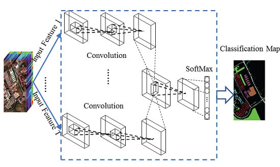
Figure 1 illustrates the structure of the proposed framework. The first step of this framework is the extraction of multiple HSI features followed by several CNN blocks. Given $T$ sets of features, each individual CNN block will learn the corresponding representative feature map, and all the feature maps will be jointed by a concatenating layer. The weight and bias for each block are fine-tuned in this network through back propagation. The output of the network for each pixel is a vector of class membership probability with $C$ units, corresponding to $C$ classes defined in the hyperspectral data set. The main principles of the proposed framework are explained in detail in the following sections.

2.1. Extraction of Attribute Profiles

The characterization of spatial contextual information computed by morphological profiles (MPs) can represent the variability of the structures for images [27]. However, features extracted by a specific MP cannot be modelled as other geometrical features. In order to model various geometrical characteristics simultaneously for the feature extraction in HSI classification, the application of attribute profiles (APs) is firstly introduced in the work of [28]. APs showed interesting properties in HSI processing, which can be used to generate an extended AP (EAP).

APs are a generalized form of MPs, which can be obtained from an image by applying a criterion $T$. The construction of APs relies on the morphological attribute filters (AFs), and it can be obtained by applying a sequence of AFs to a scalar image [28]. AFs are defined as the connected operators which process the image by merging its connected components instead of pixels. After the operators are applied to the regions, the attribute results are compared to a pre-defined reference value. The region is determined to be preserved or removed from the image depending on whether the criterion is met or not (i.e., the attribute results are preserved if the value is larger than the pre-defined reference value). The values in the removed region will be set as the closest grayscale value of the adjacent region. If the merged region is a lower (greater) gray level, then the thinning (thickening) is applied.

Subsequently, an AP can be directly constructed by using a sequence of thinning and thickening AFs which are applied to the image with a set of given criteria. By using $n$ morphological thickening (${\phi }^T$) and $n$ thinning (${\varphi }^T$) operators, an AP from the image $f$ can be constructed as:

$$\mathrm{AP}(f)=\{{\phi }_n^T(f),{\phi }_{n-1}^T(f),\mathrm{...},{\phi }_1^T(f),f,{\varphi }_1^T(f),\mathrm{...},{\varphi }_{n-1}^T(f),{\varphi }_n^T(f)\}$$

(1)

Generally, there are some common criteria associated with the operators, such as area, volume, diagonal box, and standard deviation. According to the operators (thickening or thinning) used in the image processing, the image can be transformed to an extensive or anti-extensive one. In this paper, since our goal is to measure the effectiveness of multiple feature learning by the proposed CNN, but not to achieve absolute performance maximization, only APs based on four different criterions (i.e., area, standard deviation, the moment of inertia, and length of the diagonal) are extracted as the different feature maps for classification tasks. In addition, in this paper, the different AP features are named by the corresponding criterions. One can find the details of various APs from [27].

2.2. Convolutional Neural Networks

CNNs aim to extract the representative features for different forms of data via multiple non-linear transformation architectures [29]. The features learned by a CNN are usually more reliable and effective than rules-based features. In this paper, we consider HSI classification with the so-called directed acyclic graphs (DAG) where the layers are not limited to chaining one after another. For HSI classification, a neural network can realize the function of mapping the input HSI pixels to the output pixel labels. The function is composed of a sequence of simple blocks that are called layers. The basic layers in a CNN are as follows:

Mathematically, an individual neuron is computed by taking a vector of inputs $x$ and applying an operator to it with a weight filter $f$ and bias $b$:

$$a=\sigma (fx+b)$$

(2)

where $\sigma (·)$ is a nonlinear function named as an activation function. For a convolutional layer, every neuron is related to a spatial location ($i,j$) with respect to the input image. The output $a_{i,j}$ associated with the input can be defined as follows:

$$a_{i,j}=\sigma ({(F\otimes X)}_{i,j}+b)$$

(3)

where $F$ is the kernel function with the learned weights, $X$ is the input or the layer, and $\otimes$ denotes the convolution operator. Usually at least one layer of the activation function is implemented in a network. The most frequently used activation functions are the sigmoid function and the ReLU function. The ReLU function has been considered to be more efficient than the sigmoid function in the convergence of the training procedure [29]. The ReLU function is defined as follows:

$$\sigma (x)=\max (0,x)$$

(4)

Another important type of layers is pooling which is implemented as a down-sampling function. The most common types of pooling are the max-pooling and mean-pooling. The pooling function partitions the input feature map into a set of rectangles and outputs the max/mean value for each sub-region. Hence, the computational complexity can be reduced.

Typically, a softmax function is performed in the top layer so that a probability distribution as an output can be obtained with each unit representing a class membership probability. Based on the above principle, in this paper, different features of the raw image are fed into each corresponding CNN block, and the network is fine-tuned through the back propagation.

2.3. Architecture of Convolutional Neural Network

HSI contains several hundreds of spectral bands, and the input of a HSI classifier is usually the whole image. This is different from common classification problems. It has been acknowledged that spatial contextual information extraction is essential for HSI classification. Based on such knowledge, we choose a three dimensional structure of the HSI pixel as input to the built CNN model. Given a HSI cube $X\in {ℝ}^{M\times N\times L}$, $M\times N$ is the image size and $L$ denotes the number of spectral channels. For a test pixel $x_i$ (where $i$ is the index of the test pixel), a $K\times K\times B$ format structure of this pixel will be adopted as the input with $K\times K$ being a fixed neighborhood size and $B$ representing the dimension of the input features. For example, for the original image cube, $B$ is equal to the number of the spectral channels $L$. In this paper, after $T$ attribute profile features (i.e., area, standard deviation, length of diagonal, and moment of inertia) are extracted, each attribute can be expressed as $A_t\in {ℝ}^{M\times N\times B_t}$, $t=1,2,\mathrm{...}T$. $A_t$ denotes the tth attribute of $X$, $B_t$ denotes the number of spectral channels of $A_t$. For each pixel in $A_t$, a $K\times K\times B_t$ neighborhood region patch will be chosen as the input to the corresponding model.

Each convolutional layer has a four-dimensional convolution of $W\times W\times B\times F$, where $W\times W$ is the kernel size of the convolutional layer, $B$ is the dimension of input variable and $F$ denotes the number of kernels in each convolutional layer. For example, for a $2\times 2\times 200\times 50$ convolutional layer with an input size of $5\times 5\times 200$, the output in the DAG will be a format of $4\times 4\times 50$ which will be the input of the next layer.

The three-dimensional format of the input in the proposed network makes the dimensionality around several hundreds ($K\times K\times B$), which may lead to an overfitting problem during the training procedure. In order to handle this situation, ReLU is applied to the proposed network. The adopted ReLU in this paper is a simple nonlinear function that produces 0 or 1 corresponding to the positive or negative input of a neuron. It has been confirmed that ReLU can boost the performance of networks in many cases [30].

To perform the classification with the learned representative features, a softmax operator is applied to the top layer of the proposed network. Softmax is one of the probabilistic-based classification models which measure the correlation between an output value and a reference value by a probability score. It should be noted that in the CNN construction, softmax can be applied throughout the spectral channels for all spatial locations in a convolutional manner [31]. For the given input of three dimension ($K\times K\times B$), the probability that the input belongs to class $c$ is computed as follows:

$$p(y=c)=\frac{e^{x_{mnk}}}{{\displaystyle \sum _{b=1}^B{e}^{x^{mnb}}}}$$

(5)

In order to obtain the essential probability distribution using the softmax operator, the number of kernels of the last layer should be set as the same as the number of classes defined in the HSI data set. The whole training procedure of the network can be treated as the optimization of parameters, which can minimize a loss function between the network outputs and ground truth values for the training data set. Let $y_i=1,\mathrm{...},c,\mathrm{...},C$ denote the target ground truth value corresponding to the text pixel $x_i$, and $p(y_i)$ be the output class membership distribution with $i$ as the index of the test pixel. The multi-class hinge loss used in this paper is given by

$$L={\displaystyle \sum _{i=1}^N{\displaystyle \sum _{c=1}^C\max (0,1-p(y_i=c))}}$$

(6)

Finally, the predication label is decided by taking the argmin value of the loss function:

$${\widehat{y}}_i=\underset{c}{\arg \min }L$$

(7)

3. Experimental Results and Discussion

The proposed framework was tested with three benchmark HSI data sets (The MATLAB implementation is available on request). Section 3.1 below introduces the data sets and shows the class information. Section 3.2 layouts the specific network architectures applied in this paper and other relevant information regarding the experimental evaluation. Section 3.3 provides the experimental results for all the classifiers. Section 3.4 highlights some additional experiments influential to the classification results. In this paper, the original features, as well as four attribute features extracted based on four attribute filters (i.e., area, moment of inertia, length of diagonal and standard deviation) are used as inputs to the proposed network. The parameters for each AP criterion are set as default as the ones in [28].

In order to validate the effectiveness of the proposed mechanism, the proposed work is compared with the designed CNN with original images (referred to as O-CNN), and a CNN using all features (including the original images) stacked as input (referred to as E-CNN). As shown in Figure 2, for fair comparison, these CNNs have architectures similar to the proposed network. The attribute features extracted in this paper have the parameters set as the ones in [27]. All the programs are executed in Matlab 2015b. The test is conducted on Intel (R) Core (TM) i7-4790 CPU 3.60 GHz and 16 GB Installed Memory. All the convolutional network models are implemented based on the publicly available matconvnet [31] with some modifications, and the optimization algorithms used in this paper are implemented by the Statistics and Machine Learning Toolbox in Matlab.

3.1. Data Description

To verify the effectiveness of the proposed framework, three benchmark data sets [32] are used in this paper:

• Airborne Visible/Infrared Imaging Spectrometer (AVIRIS) data set: Indian Pines. It was obtained by the AVIRIS sensor over the site in northwest Indiana, United States of America (USA). This imagery has 16 labeled classes. The data set has 220 spectral bands ranging from 0.2 to 2.4 µm wavelength, and each channel has 145 × 145 pixels with a spatial resolution of 20 m. 20 water absorption bands are removed during the experiments.
• Reflective Optics System Imaging Spectrometer (ROSIS) data set: University of Pavia, Italy. This image was acquired over Pavia in north Italy. It has nine labeled ground truths with 610 × 610 pixels. Each pixel has a 1.3 m spatial resolution. With water absorption bands removed, 103 bands are used in the experiment.
• AVIRIS data set: Salinas. This image was also acquired by the AVIRIS sensor over Salinas Valley, California, USA. The image is of 512 × 217 pixels, and with 224 spectral bands. The Salinas data has a 3.7 m resolution per pixel and 16 different classes. The ground truth and false color images for the data sets are illustrated in Figure 3.

For each of the three data sets, the samples are split into two subsets, i.e., a training set and a test set. The details of the number of the subsets are listed in

Table 1. Class Information for Indian Pines Data Set.

No.	Class Name	Training	Test
1	Alfalfa	30	16
2	Corn-no till	250	1178
3	Corn-min till	250	580
4	Corn	150	87
5	Grass/trees	250	233
6	Grass/pasture	250	480
7	Grass/pasture-mowed	20	8
8	Hay-windrowed	250	228
9	Oats	15	5
10	Soybeans-no till	250	722
11	Soybeans-min till	250	2205
12	Soybeans-clean till	250	343
13	Wheat	150	55
14	Woods	250	1015
15	Buildings-grass-trees	50	336
16	Stone-steel towers	50	43
Total		2715	7534

,

Table 2. Class Information for University of Pavia Data Set.

No.	Class Name	Training	Test
1	Asphalt	250	6381
2	Meadows	250	18,399
3	Gravel	250	1849
4	Trees	250	2814
5	Meta sheets	250	1095
6	Bare soil	250	4779
7	Bitumen	250	1080
8	Bricks	250	3432
9	Shadows	250	697
Total		2250	40,526

and

Table 3. Class Information for Salinas Data Set.

No.	Class Name	Training	Test
1	Weeds_1	300	1709
2	Weeds_2	300	3426
3	Fallow	300	1676
4	Fallow plow	300	1094
5	Fallow smooth	300	2378
6	Stubble	300	3659
7	Celery	300	3279
8	Grapes	300	10,971
9	Soil	300	5903
10	Corn	300	2978
11	Lettuce 4 week	300	768
12	Lettuce 5 week	300	1627
13	Lettuce 6 week	300	616
14	Lettuce 7 week	300	770
15	Vineyard untrained	300	6968
16	Vineyard trellis	300	1507
Total		4800	49,329

. For training the architecture of each CNN block, 90% of the training pixels are used to learn the filter parameters for each CNN block and the remaining 10% are used as the validation set. The training set is used to adjust the weights on the neural network. The validation set is used to provide an unbiased evaluation of a model fit on the training data set, which means that this data set is predominately used to describe the evaluation of models when tuning hyper parameters. The test is used only to assess the performance of a fully-trained CNN model.

3.2. Network Design and Experimental Setup

CNN blocks for different features were designed to have the same architecture. There are three convolutional layers, pooling layers, ReLU layers and concatenating layers. The details of the network structure are listed in

Table 4. Network Structure for Indian Pines Data Set.

Input Features	Layer No.	Convolution	ReLU	Pooling
Original image	1	2 × 2 × 200 × 200	No	2 × 2
	2	(Transpose) 2 × 2 × 200 × 200	Yes	No
AP (Area)	1	2 × 2 × 125 × 200	No	2 × 2
	2	(Transpose) 2 × 2 × 200 × 200	Yes	No
AP (Length of diagonal)	1	2 × 2 × 175 × 200	No	2 × 2
	2	(Transpose) 2 × 2 × 200 × 200	Yes	No
AP (Moment of inertia)	1	2 × 2 × 75 × 200	No	2 × 2
	2	(Transpose) 2 × 2 × 200 × 200	Yes	No
AP (Standard deviation)	1	2 × 2 × 75 × 200	No	2 × 2
	2	(Transpose) 2 × 2 × 200 × 200	Yes	No
	Concatenating	Dim = 2 (Horizontal)
	Convolution	4 × 2$0 \times$200 × 16

,

Table 5. Network Structure for University of Pavia Data Set.

Input Features	Layer No.	Convolution	ReLU	Pooling
Original image	1	4 × 4 × 103 × 200	No	2 × 2
	2	(Transpose) 2 × 2 × 200 × 200	Yes	No
AP (Area)	1	4 × 4 × 20 × 200	No	2 × 2
	2	(Transpose) 2 × 2 × 200 × 200	Yes	No
AP (Length of diagonal)	1	4 × 4 × 103 × 200	No	2 × 2
	2	(Transpose) 2 × 2 × 200 × 200	Yes	No
AP (Moment of inertia)	1	4 × 4 × 12 × 200	No	2 × 2
	2	(Transpose) 2 × 2 × 200 × 200	Yes	No
AP (Standard deviation)	1	4 × 4 × 12 × 200	No	2 × 2
	2	(Transpose) 2 × 2 × 200 × 200	Yes	No
	Concatenating	Dim = 2 (Horizontal)
	Convolution	4 × 2$0 \times$200 × 9

and

Table 6. Network Structure for Salinas Data Set.

Input Features	Layer No.	Convolution	ReLU	Pooling
Original image	1	6 × 6 × 224 × 200	No	2 × 2
	2	(Transpose) 2 × 2 × 200 × 200	Yes	No
AP (Area)	1	6 × 6 × 15 × 200	No	2 × 2
	2	(Transpose) 2 × 2 × 200 × 200	Yes	No
AP (Length of diagonal)	1	6 × 6 × 21 × 200	No	2 × 2
	2	(Transpose) 2 × 2 × 200 × 200	Yes	No
AP (Moment of inertia)	1	6 × 6 × 9 × 200	No	2 × 2
	2	(Transpose) 2 × 2 × 200 × 200	Yes	No
AP (Standard deviation)	1	6 × 6 × 9 × 200	No	2 × 2
	2	(Transpose) 2 × 2 × 200 × 200	Yes	No
	Concatenating	Dim = 2 (Horizontal)
	Convolution	4 × 2$0 \times$200 × 16

. The input images are initially normalized into [−1 1]. The number of kernels in each convolutional layer is set as 200 empirically. The input neighborhood of each feature is set as 5 × 5, 7 × 7 and 9 × 9 for the Indian Pines data set, the University of Pavia data set and the Salinas data set, respectively. The learning rate for CNN models is set as 0.01; the number of epochs is set as 100 for the Indian Pines and the University of Pavia data sets, and 150 for the Salinas data set. The batch size is set as 10. To quantitatively validate the results of the proposed framework, overall accuracy (OA), average accuracy (AA) and the Kappa coefficient ($k$) are adopted as the performance metrics. Each result is shown as an average of ten times repeated experiments with the randomly chosen training samples.

3.3. Experimental Results and Discussion

3.3.1. Classification Results for the Indian Pines Data Set

Table 7. Classification Results (%) of Indian Pines Data Set.

Class No.	O-CNN	E-CNN	Proposed
1	95.65	97.83	97.83
2	87.96	95.52	94.82
3	93.86	85.66	97.23
4	98.73	100.00	99.58
5	98.14	95.24	99.59
6	97.53	95.48	99.59
7	100.00	92.86	100.00
8	98.12	100.00	100.00
9	100.00	100.00	100.00
10	90.02	88.17	93.93
11	74.95	89.41	97.23
12	91.40	93.25	98.99
13	100.00	97.07	100.00
14	94.62	96.84	99.76
15	95.34	98.70	97.93
16	100.00	94.62	98.92
OA	89.14	93.04	97.57*
AA	94.77	95.04	98.46*
k	87.73	92.11	97.23*

* The bold style represents the highest accuracy among the compared methods.

shows the classification results obtained by different classifiers for the Indian Pines data set, and the resultant maps are provided in Figure 4. One can observe that all the CNN-based models achieve a good performance, and the proposed method provides the improved results on this data set. For O-CNN, the original image is set as the input for the network. In order to verify the effectiveness of the proposed mechanism, the spatial contextual features are extracted and stacked together to be fed into the network for E-CNN. E-CNN has achieved more accurate results than O-CNN, but failed to outperform the proposed method. The best performance achieved by the proposed framework is probably due to the joint exploitation of spatial-spectral information. One can conclude that the proposed method produces less “salt-and-pepper” noise on the classification maps. In comparison with O-CNN, OA, AA and Kappa of the proposed method are improved by 8.43%, 3.69% and 9.5%. The same conclusion can be made when the proposed method is compared with E-CNN, especially the improvement is quite significant for the sets of similar class labels as can be observed from Table 7. For example, the accuracies obtained by the proposed method for the classes Soybeans-no till, Soybeans-min till and Soybeans-clean till (class no. 10, 11, and 12) are 5.76%, 7.82% and 5.74% higher than those obtained by the E-CNN. The same conclusion can be obtained when the individual class accuracies for the similar sets of Grass-tress, Grass-pasture and Grass-pasture mowed (class no. 5, 6, and 7) are inspected. The results show that the proposed algorithm has a very competitive ability in classifying the similar and mixed pixels. In addition, the proposed method has demonstrated the best performance in terms of preserving the discontinuities which can be observed from the classification maps. Moreover, CNN methods do not need predefined parameters whereas pixel-level extraction methods require them.

3.3.2. Classification Results of the University of Pavia Data Set

The class-specific classification accuracies for the University of Pavia image and the representative classification maps are provided in

Table 8. Classification Results (%) of University of Pavia Data Set.

Class No.	O-CNN	E-CNN	Proposed
1	97.50	99.68	99.25
2	94.38	99.93	99.74
3	96.62	94.46	99.76
4	97.58	97.35	99.64
5	100.00	100.00	100.00
6	93.52	97.82	99.96
7	93.16	98.57	98.80
8	93.10	98.38	99.48
9	99.68	99.79	99.89
OA	95.25	98.99	99.64 *
AA	96.17	98.44	99.61 *
k	93.75	98.67	99.53 *

* The bold style represents the highest accuracy among the compared methods.

and Figure 5, respectively. From the results, one can see that the proposed method outperforms the other algorithms in terms of OA, AA and Kappa. The proposed method significantly improves the results with a very high accuracy when tested with the University of Pavia data set. From the illustrative results in classification maps, O-CNN and E-CNN show more noisy scattered points in the images. The proposed method can remove them and lead to smoother classification results without blurring the boundaries.

3.3.3. Classification Results of the Salinas Data Set

Table 9. Classification Results (%) of Salinas Data Set.

Class No.	O-CNN	E-CNN	Proposed
1	100.00	100.00	100.00
2	99.84	99.92	99.92
3	99.60	99.70	99.65
4	99.57	99.93	99.78
5	99.93	99.78	99.07
6	99.95	100.00	99.97
7	99.30	99.92	99.75
8	95.52	95.73	94.28
9	99.45	100.00	99.97
10	97.32	99.73	99.63
11	99.53	100.00	99.91
12	100.00	100.00	100.00
13	100.00	100.00	100.00
14	100.00	100.00	99.91
15	66.29	81.65	97.40
16	95.35	100.00	100.00
OA	94.06	96.60	98.34 *
AA	96.98	98.52	99.33 *
k	93.37	96.20	98.15 *

* The bold style represents the highest accuracy among the compared methods.

shows the classification results for the Salinas data set with different classifiers, and the classification accuracies are illustrated in Figure 6. The results are similar to the previous two data sets. Under the condition of the same training samples, the proposed method outperforms the other approaches in terms of OA, AA and Kappa. Although E-CNN improved the classification results of O-CNN by stacking different features, the improvement is limited when compared to the proposed framework. The better performance of the proposed network proves the capacity and effectiveness of the built network for multiple feature learning.

3.4. Discussion of Effects of Different Parameters

3.4.1. The Impact of the Number of Training Epochs

The number of training epochs is an important parameter for the CNN-based methods. Figure 7 shows that the training error varies with the number of training epochs on all three data sets. In the training process for a network, the back propagation is implemented by minimizing the training error “objective” which is computed by $objective=-{\displaystyle \sum _{i=1}^{N_t}log(p_{ic})}$ Here, the trend of the “error” item is computed by $error={\displaystyle \sum _{i=1}^{N_t}{p}_{ic}(argmax{p}_i\sim =c)}$ where N_t denotes the number of training samples, p_ic denotes the cth prediction probability of the training pixel x_i which belongs to the cth class. It is helpful and useful for assessment. From Figure 7, one can observe that it converges faster for the training process of the Indian Pines image and the University of Pavia image, slower for the Salinas image. ReLU is an important factor which is influential to the training procedure; ReLU can accelerate the convergence of the network and improve the training efficiency [29].

3.4.2. The Impact of Training Samples

One critical factor to the training a CNN is the number of training samples. It is widely known that a CNN may not extract effective features unless abundant training samples are available. However, it is not common for HSI to have a large number of training samples, hence it is very important to build a network that is robust and efficient for the classification task.

In this paper, the impacts of the number of training samples on the accuracies of three data sets are also tested. For the Indian Pines scene, 5 to 50% of the samples are randomly selected as training pixels and the remaining pixels are used as the test set. For both the University of Pavia and the Salinas images, 50 to 500 pixels per class are chosen randomly as the training samples with the remaining as the test set. 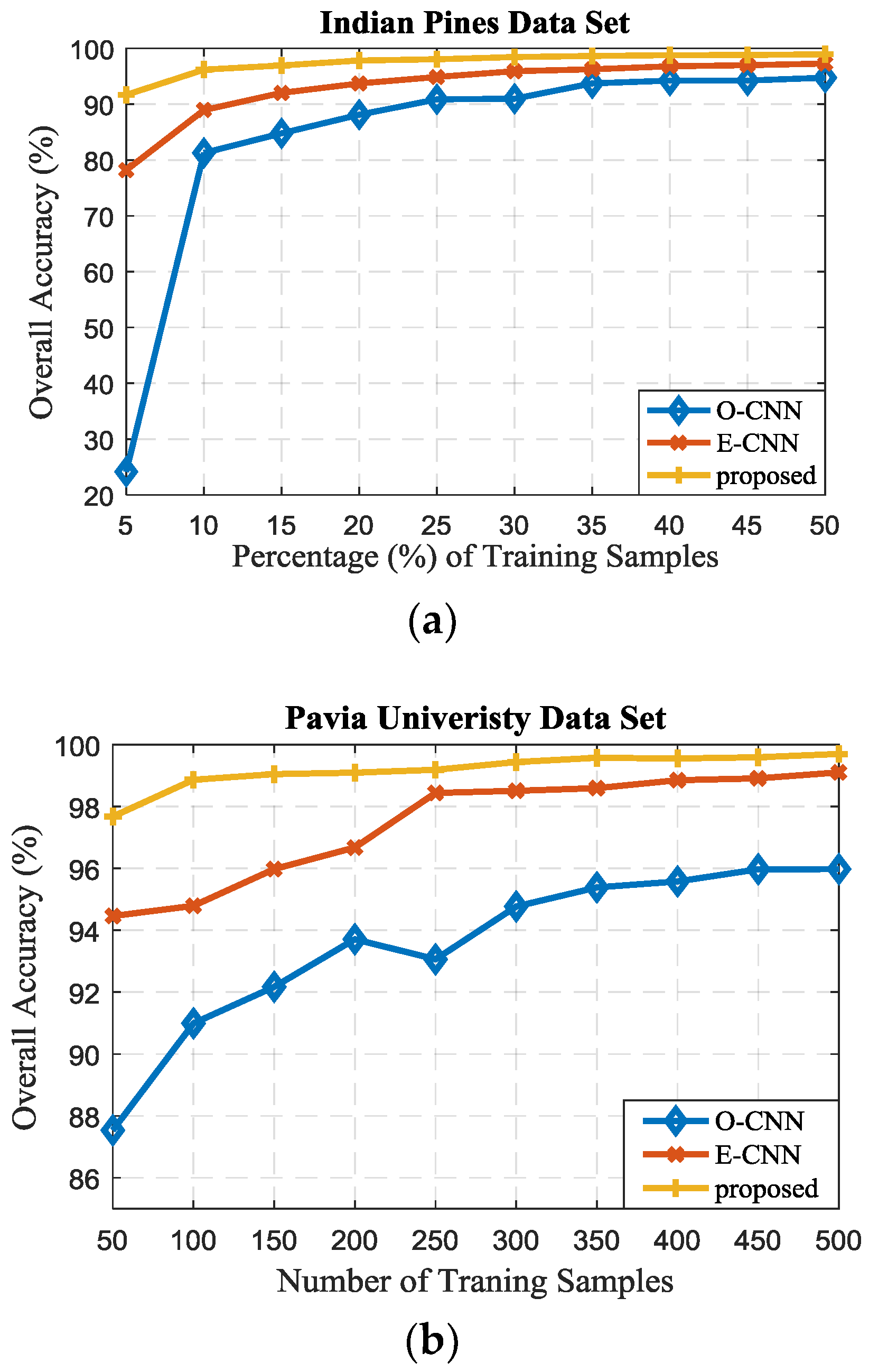Figure 8 illustrates the OA for various methods with different numbers of training pixels. From Figure 8, one can see that all the methods perform better if the number of training samples increases for the Indian Pines data set, and the proposed method performs the best. Especially, the proposed method obtains an accuracy of higher than 95% with less than 10% training samples. The accuracies tend to become stabilized for these three methods if the number of training samples further increases. For the University of Pavia data set, the classification accuracies for these CNN-based methods show approximately 100% as the number of training samples further increases, especially for the proposed method which has the accuracy more than 96% with 50 samples per class. For the Salinas data set, the performances for all approaches fluctuate in a range, and the proposed method performs the best in most cases. It should be noted that for the whole three data sets, the CNN-based classifiers are more sensitive to the number of training samples and the accuracy increases as the number of training samples increases. In addition, the CNN-based approaches can achieve a competitive performance with a large number of training samples, and the proposed method shows more robustness with a variety of the number of training samples.

3.4.3. The Impact of Input Neighborhood Size

The neighborhood size $K\times K$ of the input image is another important factor related to the classification results. Figure 9 illustrates the network architectures with inputs of different neighborhood sizes. The only difference for the three data sets is the number of kernels in the last layer, which is 16 for the Indian Pines and the Salinas data sets, and 9 for the University of Pavia data set. It should be noted that, in order to obtain the probability scores corresponding to different classes, the number of kernels in the last layer should be the number of labeled classes for each data set. In Figure 9, we take the University of Pavia data set as an example. As shown in

Table 10. Classification Results (%) of Indian Pines Data Set using Network with Inputs of Different Neighborhood Sizes.

	5 × 5	7 × 7	9 × 9	11 × 11
OA	97.57	97.19	95.24	93.61
AA	98.46	98.05	96.12	94.28
k	97.23	96.80	94.58	92.71

,

Table 11. Classification Results (%) of University of Pavia Data Set using Network with Inputs of Different Neighborhood Sizes.

	5 × 5	7 × 7	9 × 9	11 × 11
OA	99.19	99.64	99.60	99.49
AA	99.38	99.74	99.63	99.61
k	98.92	99.53	99.33	99.47

and

Table 12. Classification Results (%) of Salinas Data Set using Network with Inputs of Different Neighborhood Sizes.

	5 × 5	7 × 7	9 × 9	11 × 11
OA	95.97	97.38	98.34	97.82
AA	98.42	98.90	99.33	99.16
k	95.53	97.09	98.15	97.58

, the performances decrease with the neighborhoods up to 7 × 7, 9 × 9 and 11 × 11 for three data sets, respectively. The performance degradation may be caused by the “over-smoothing” effect across the boundaries as the neighborhood size increases. Hence, 5 × 5, 7 × 7 and 9 × 9 are the optimal neighborhood sizes for the three data sets in the proposed network.

3.4.4. The Analysis of Multiple Feature Learning

To verify the effectiveness of the multiple feature learning, the experimental results for the designed CNN (Figure 2a) with individual features (i.e., area, moment of inertia, length of diagonal and standard deviation) are also shown in

Table 13. Classification Results (%) for Individual AP Features of Indian Pines Data Set.

Accuracy	AP (Area)	AP (Length of Diagonal)	AP (Moment of Inertia)	AP (Standard Deviation)
OA	94.43	95.58	94.96	92.77
AA	96.85	96.60	96.83	95.66
k	93.67	94.18	94.26	91.78

,

Table 14. Classification Results (%) for Individual AP Features of University of Pavia Data Set.

Accuracy	AP (Area)	AP (Length of Diagonal)	AP (Moment of Inertia)	AP (Standard Deviation)
OA	93.20	98.47	95.82	91.77
AA	95.93	98.52	97.35	94.28
k	91.14	98.31	94.49	89.26

and

Table 15. Classification Results (%) for Individual AP Features of Salinas Data Set.

Accuracy	AP (Area)	AP (Length of Diagonal)	AP (Moment of Inertia)	AP (Standard Deviation)
OA	93.59	96.29	93.45	92.39
AA	96.76	97.43	96.73	96.16
k	92.85	95.88	92.68	91.50

for the validation. From these tables, one can see that the designed CNN with features of length of diagonal performs better than other networks. Compared with the results in Table 7, Table 8 and Table 9, it is obvious that E-CNN compromises the accuracy for the classification. This may be due to the data augmentation caused by the initial concatenation which is not proper for the spatial filter. The higher accuracy obtained by the proposed method benefits from the joint exploitation in the processing stage where the dimension has been cut off by the spatial filter. In addition, the concatenation of the various features at first step of E-CNN may lose the discriminative information during the training process. The various features possess different properties, learnt through the individual convolutional layers can help extract the better feature representations for the classification which leads to a superior performance. The proposed joint structure-based multi-feature learning can adaptively learning the heterogeneity of each feature, and eventually result in a better performance. It can be concluded that the comparison results with individual features reveal the effectiveness of the multiple feature learning technique of the proposed method.

3.4.5. Training Time

The training and test time averaged over ten repeated experiments for the three data sets are given in

Table 16. Training/Test Time (minutes) Averaged over Ten Time Repeatedly Experiments on Three Data Sets for Different Classifiers.

	O-CNN Training/Test	E-CNN Training/Test	Proposed Training/Test
Indian Pines	8.7/0.74	9.7/0.8	17.1/1.5
University of Pavia	17.2/1.9	27.5/2.1	38.8/3.9
Salinas	42.8/4.5	45.6/5.2	66.1/10.2

. The training procedure for a CNN is time-consuming; however, another advantage of CNN algorithms is that they are fast for testing. In addition, the training time would take just a few seconds with GPU processing.

4. Conclusions

In order to prove the potential of CNNs for HSI classification, we presented a framework consisting of a novel CNN model. The framework was designed to have several individual CNN blocks with comprehensive features as input. To enhance the learning efficiency as well as to leverage both the spatial contextual and spectral information of the HSI, the output feature maps of each block are then concatenated and fed into subsequent convolutional layers to derive the pixel label vectors. By using the proper architecture, the built network is a shallow but efficient one, and it can concurrently exploit the interactions of different spectral and spatial contextual information by using the concatenating layer. In comparison with the CNN-based single feature learning method, the classification results are improved significantly with multiple features involved. Moreover, in contrast to the traditional rule-based classifiers, the CNN-based framework can extract the deep features automatically and in a more efficient way.

Moreover, the experiments suggest that a three-layer CNN is optimal for HSI classification, and the neighborhood size between 2 × 2 to 6 × 6 can balance the efficiency and complexity of the network. The pooling layer with a size of 2 × 2 and 200 kernels in each layer can provide an enough capacity for the network. Since the training samples are very limited in HSI classification, the multiple input feature maps and ReLU in the proposed network can help alleviate the overfitting phenomenon and accelerate convergence. The tests with three benchmark data sets showed superior performances of the proposed framework. As CNNs are gaining attention due to the strong ability in extracting the relevant features for image classification, the proposed method is expected to provide various improvements for the better feature representation purpose.