Deriving Total Suspended Matter Concentration from the Near-Infrared-Based Inherent Optical Properties over Turbid Waters: A Case Study in Lake Taihu

Abstract

Normalized water-leaving radiance spectra nL_w(λ), particle backscattering coefficients b_bp(λ) in the near-infrared (NIR) wavelengths, and total suspended matter (TSM) concentrations over turbid waters are analytically correlated. To demonstrate the use of b_bp(λ) in the NIR wavelengths in coastal and inland waters, we used in situ optics and TSM data to develop two TSM algorithms from measurements of the Visible Infrared Imaging Radiometer Suite (VIIRS) onboard the Suomi National Polar-orbiting Partnership (SNPP) using backscattering coefficients at the two NIR bands b_bp(745) and b_bp(862) for Lake Taihu. The correlation coefficients between the modeled TSM concentrations from b_bp(745) and b_bp(862) and the in situ TSM are 0.93 and 0.92, respectively. A different in situ dataset acquired between 2012 and 2016 for Lake Taihu was used to validate the performance of the NIR TSM algorithms for VIIRS-SNPP observations. TSM concentrations derived from VIIRS-SNPP observations with these two NIR b_bp(λ)-based TSM algorithms matched well with in situ TSM concentrations in Lake Taihu between 2012 and 2016. The normalized root mean square errors (NRMSEs) for the two NIR algorithms are 0.234 and 0.226, respectively. The two NIR-based TSM algorithms are used to compute the satellite-derived TSM concentrations to study the seasonal and interannual variability of the TSM concentration in Lake Taihu between 2012 and 2016. In fact, the NIR-based TSM algorithms are analytically based with minimal in situ data to tune the coefficients. They are not sensitive to the possible nL_w(λ) saturation in the visible bands for highly turbid waters, and have the potential to be used for estimation of TSM concentrations in turbid waters with similar NIR nL_w(λ) spectra as those in Lake Taihu.

1. Introduction

Total suspended matter (TSM) is an important biogeochemical parameter for both the ocean environment and inland waters. It can significantly impact the light fields in the water column, and consequently affect water optical and biological properties, such as the diffuse attenuation coefficient at the wavelength of 490 nm K_d(490) [1,2,3], chlorophyll-a (Chl-a) concentration [4,5,6], and primary production [7,8], etc. TSM is also an indicator of water quality and water clarity that can affect both aquatic life and the lives of millions of people near coastal and inland waters. Changes in TSM concentrations are also related to the different atmosphere, land, and ocean processes, such as river runoff and discharge [9,10], landslides and erosion [11], hurricanes and tropical storms [12,13,14], and ocean tidal currents [15,16].

In recent years, satellite ocean color remote sensing has been increasingly used to study ocean optical, biological, and biogeochemical processes, as well as to monitor for natural hazards in the world’s open oceans and coastal and inland waters. Several algorithms have already been developed to derive the TSM concentration from satellite-measured normalized water-leaving radiance spectra nL_w(λ). Specifically, nL_w(λ) at the wavelength of 645 nm from the Moderate Resolution Imaging Spectroradiometer (MODIS) can be used to map TSM concentrations [17]. Remote sensing reflectance retrievals at wavelengths of 545 and 840 nm from Satellite Pour l’Observation de la Terre (SPOT) data have been used to quantify the TSM concentration [18]. Using MODIS-Aqua measurements, Son and Wang [19] developed a TSM algorithm for Chesapeake Bay using the strong relationship between TSM and the water diffuse attenuation coefficient at 490 nm (K_d(490)). Tassan [20] computed TSM using remote sensing reflectance at wavelengths of 488, 555, and 645 nm from Landsat Thematic Mapper (TM) data, and it was further tuned for MODIS observations in the Yellow Sea and East China Sea [21]. Other TSM algorithms, which are empirically tuned with different statistical approaches, were also developed for the Yellow Sea and East China Sea [22,23].

In general, our knowledge of the optical features in the red (~620–700 nm), near-infrared (NIR, ~700–1000 nm), and shortwave infrared (SWIR, ~1000–3000 nm) wavelengths for the coastal and inland waters is still quite limited, particularly for optical information at the NIR and SWIR wavelengths. Though, the optical information in the red, NIR, and SWIR can be used to derive a variety of ocean (water) products in turbid coastal and inland waters to address dynamic coastal ocean and inland water environments [24,25,26,27].

The water inherent optical properties (IOPs) are important parameters of the absorption and scattering of the constituents in the water column, i.e., pure water, phytoplankton, color dissolved organic matter (CDOM), and minerals, etc. It is well known that nL_w(λ) spectra are determined by IOPs, such as absorption and backscattering of different bio-physical components in the water column [28]. Thus, IOPs can be derived using nL_w(λ) spectra from satellite remote sensing [29,30,31]. However, most of these studies are focused on open ocean and less turbid waters. In fact, only nL_w(λ) spectra in the visible are used in these IOP retrieval algorithms. The performance of these algorithms is poor in turbid coastal and inland waters since the coefficeints for IOP spectral relations are empirical and normally tuned for open oceans or less turbid waters. In addition, the saturation of nL_w(λ) in the visible wavelengths [32,33] in the highly turbid waters also indicates that IOP retrievals with nL_w(λ) in the visible wavelengths can lead to significant underestimation of IOPs. Recently, improvements were also made to tune these algorithms with the in situ nL_w(λ) in the NIR wavelengths in some regional studies [34,35,36].

In turbid coastal and inland waters, the backscattering coefficient b_bp(λ) is generally proportional to the TSM concentration, thus deriving b_bp(λ) becomes a prerequisite for any IOP-based TSM algorithm. In the visible wavelengths, the absorption and backscattering of all four constituents in the water column are significant in determining the nL_w(λ) spectra. This makes it very challenging to accurately derive IOP properties from satellite-measured nL_w(λ) spectra with visible bands in the coastal and inland waters. However, at the NIR wavelengths, the water absorption coefficients [37,38] are much larger than those of other components, such as phytoplankton, sediments, and CDOM. Thus, IOP models at the NIR wavelengths can be significantly simplified for turbid coastal and inland waters [33]. Indeed, Shi and Wang [33] have shown that backscattering coefficients b_bp(λ) at the MODIS NIR bands can be analytically derived with good accuracy at the NIR and visible wavelengths in coastal and inland waters. The NIR-based algorithm also has the potential to further extend to the visible bands to derive the IOP properties, such as a_ph(λ), a_cdom(λ) over turbid coastal and inland waters.

In this paper, we further demonstrate that the NIR-based backscattering coefficients derived from the Visible Infrared Imaging Radiometer Suite (VIIRS) onboard the Suomi National Polar-orbiting Partnership (SNPP) can be used to accurately compute TSM concentrations due to the intrinsic relationship between the sediment particle backscattering coefficients and the TSM concentration. For this purpose, we use in situ measurements of the TSM and nL_w(λ) data in Lake Taihu to develop a set of the NIR-based TSM algorithms for VIIRS-SNPP applications in China’s Lake Taihu. The accuracy of these algorithms is assessed using statistical analysis. Following the TSM algorithm development, VIIRS measurements from 2012 to 2016 are processed to derive nL_w(λ) spectra using the SWIR-based atmospheric correction [39] with VIIRS SWIR M8 and M10 bands (1238 and 1601 nm). Particle backscattering coefficients at the two VIIRS NIR bands 745 and 862 nm, b_bp(745) and b_bp(862), are then calculated. We apply this set of the VIIRS TSM algorithms to derive TSM data over Lake Taihu in the VIIRS period. Furthermore, VIIRS-derived TSM data in Lake Taihu are validated using in situ TSM measurements in the VIIRS period. Finally, time series and seasonal variability of TSM concentrations in Lake Taihu are derived and analyzed.

2. Data and Method

2.1. China’s Lake Taihu

Lake Taihu is located in the Yangtze River Delta (Figure 1) with an areal coverage of ~2300 km² and a mean depth of ~2 m. Waters in Lake Taihu are consistently turbid all year with winter and summer ranking the most and least turbid seasons in the lake [40,41,42]. In addition, Lake Taihu has frequent algal blooms in the spring-summer that pollute the lake water. MODIS-Aqua observations were used to monitor the development of the blue-green algae (Microcystis) in the spring of 2007 [40] that adversely affected the normal lives of several million residents. As the third-largest inland freshwater lake in China, Lake Taihu has experienced significant environmental issues in recent years [43]. Studies have shown that the 2007 drinking water crisis is linked to climate variability and lake management [44]. In addition to the TSM and turbidity in Lake Taihu, other environmental and water quality parameters, such as phytoplankton and algal blooms [45], lake eutrophication [46], Chl-a and primary production variations [47], and CDOM [48,49] have also been investigated.

It is noted that Lake Taihu is featured with high turbidity with the K_d(490) values generally over ~2 m⁻¹, and reaching ~3–4 m⁻¹ in the winter and spring seasons for most part of the lake [40]. This shows that Lake Taihu is an optically-deep water body with negligible bottom effects on the satellite-measured nL_w(λ) spectra. On the other hand, the water absorption is significantly larger at the NIR wavelengths than that at visible wavelengths. This further suggests that the lake is optically deep and negligible bottom effects at the VIIRS NIR bands even though the bottom reflection might sometime exist for the visible bands in some regions, such as a small portion of the southeast Lake Taihu with shallower depths and low water turbidity.

2.2. In Situ Measurements of nL_w(λ) and TSM Concentration

To develop the TSM algorithms for VIIRS observations, we used the in situ measurements of nL_w(λ) and TSM concentrations between 2006 and 2007 in Lake Taihu. In that period, five cruises were carried out to collect optical measurements and water samples for biological and bio-optical properties. There were about 50 sample stations covering the entire area of Lake Taihu for each cruise. The time periods for the five cruises were 7–9 January 2006, 29 July–1 August 2006, 12–15 October 2006, 7–9 January 2007, and 25–27 April 2007. The optical and biogeochemical parameters from the in situ measurements at each station include hyperspectral remote sensing reflectance for wavelengths between 350 and 1050 nm and TSM concentration.

The optical measurements were made, and the water samples were collected, at a depth of 50 cm below the surface, comprising a total of 50 sites covering different regions of the lake. In order to obtain high-quality in situ remote sensing reflectance, measurements were carried out under clear sky conditions with no wind or very low winds during the hours of 8:30–16:30. At each sampling site, the spectra were measured 10 times to optimize the signal-to-noise ratio (SNR), and thus reduce the error of in situ measurements. Downwelling radiance and upwelling total radiance measurements were made with an ASD field spectrometer (Analytical Devices, Inc., Boulder, CO, USA) with a spectral response of 350 to 1050 nm, a spectral resolution of 3 nm, and a sampling interval of 1 nm. The water-leaving radiance L_w(λ, 0⁺) was derived after deducting the contribution of sky radiance L_sky(λ). The remote sensing reflectance above the water surface R_rs(λ) was calculated as the ratio of water-leaving upwelling radiance L_w(λ, 0⁺) to incident downwelling irradiance E_d(λ, 0⁺). The detailed protocols of the in situ data collection and processing can be found in [50,51].

In the VIIRS period between 2012 and 2016, frequent in situ measurements of TSM concentrations at a number of monitoring stations in Lake Taihu were taken. These monitoring stations were set up by the Nanjing Institute of Geography and Limnology, Chinese Academy of Sciences, aiming to monitor and assess long-term ecosystem changes in Lake Taihu. The TSM in situ measurements coincident with the VIIRS observations between 2012 and 2016 were used to validate the VIIRS-derived TSM retrievals.

2.3. VIIRS-SNPP Data and Ocean Color Data Processing

VIIRS-SNPP was launched on 28 October 2011. VIIRS has 22 spectral bands covering a spectral range from 0.410 to 12.013 µm, which include 14 reflective solar bands (RSBs), seven thermal emissive bands (TEBs), and a panchromatic day/night band (DNB) [52]. VIIRS has similar spectral bands as MODIS, which provide observations of Earth’s atmosphere, land, and ocean properties [53]. One of the primary goals of the VIIRS mission is to provide data continuity from MODIS for the science and user community with Environmental Data Records (EDR) over global oceanic waters to enable assessment of climatic and environmental variability [54]. Ocean color EDR is a key product suite derived from VIIRS [55].

Specifically, VIIRS-SNPP has five visible bands (M1–M5) with nominal central wavelengths of 410, 443, 486, 551, and 671 nm, two NIR bands (M6 and M7) at wavelengths of 745 and 862 nm, and three SWIR bands (M8, M10, and M11) at wavelengths of 1238, 1601, and 2257 nm for satellite ocean color data processing. Note that VIIRS band wavelengths are indicated for the band nominal center wavelength. In addition, effective band center wavelengths can also be calculated for the VIIRS-SNPP in order to remove the sensor out-of-band (OOB) effects following the approach in Wang at al. [56]. On-orbit vicarious calibrations for VIIRS-SNPP were carefully carried out using the in situ nL_w(λ) spectra from the Marine Optical Buoy (MOBY) [57] in waters off Hawaii and over the South Pacific Gyre (SPG) [58]. Similar to the standard NIR atmospheric correction algorithm [59,60] with two NIR bands (745 and 862 nm for VIIRS), the SWIR-based atmospheric correction algorithm with VIIRS SWIR 1238 and 1601 nm bands has been used in deriving the nL_w(λ) spectra [39]. The SWIR atmospheric correction algorithm is based on the fact that the waters are more strongly absorbing at the SWIR wavelengths than those at the NIR wavelengths [37]. Thus, normally-not-black turbid waters in the NIR bands can still be black for the SWIR bands [32,39]. Consequently, VIIRS measurements at the SWIR bands can be used to determine the aerosol type and estimate the atmospheric effects in the visible and NIR by extrapolating the aerosol effect from the SWIR wavelengths to visible and NIR wavelengths using appropriate aerosol models [39].

The Multi-Sensor Level-1 to Level-2 (MSL12), which is the official NOAA VIIRS ocean color data processing system, has been used for processing satellite ocean color data from Sensor Data Records (SDR) (or Level-1B) to ocean color EDR (or Level-2) products for VIIRS-SNPP. In recent years, MSL12 has made several important improvements and enhancements. In particular, these improvements and updates include the SWIR-based and NIR-SWIR combined atmospheric correction algorithms for improved ocean color data products in coastal and inland waters [39,61,62]. In this study, VIIRS-SNPP observations over Lake Taihu made between 2012 and 2016 were processed using the MSL12 ocean color data processing system to produce nL_w(λ) at the visible and NIR bands. Several studies have shown that MSL12 can produce good quality nL_w(λ) spectra in both open oceans and coastal regions from various satellite ocean color sensors, e.g., MODIS-Aqua, VIIRS-SNPP, and the Korean Geostationary Ocean Color Imager (GOCI) [26,40,55,62].

2.4. The NIR-IOP-Based TSM Algorithm

As a pre-requisite, b_bp(λ) data at the NIR wavelengths are required in order to derive the TSM concentration. To calculate the b_bp(λ), satellite-derived remote sensing reflectance R_rs(λ) is converted to subsurface remote sensing reflectance r_rs(λ) [63] by:

$$r_{rs}(\lambda )=\frac{R_{rs}(\lambda )}{(0.52+1.7R_{rs}(\lambda ))}$$

(1)

Gordon et al. [28] have shown that subsurface remote sensing reflectance r_rs(λ) can be computed quadratically with ocean IOPs based on the reflectance model, i.e.:

$$r_{rs}(\lambda )=g_1\left(\frac{b_b(\lambda )}{(a(\lambda )+b_b(\lambda ))}\right)+g_2{\left(\frac{b_b(\lambda )}{(a(\lambda )+b_b(\lambda ))}\right)}^2$$

(2)

where r_rs(λ) is the remote-sensing reflectance just beneath the water surface, and g₁ and g₂ are constant values of 0.0949 and 0.0794, respectively.

In comparison with nL_w(λ) results in visible bands, which are usually used for IOP modeling, pure seawater absorption coefficients a_w(λ) at the NIR bands are significantly larger than those of other seawater constituents [37], i.e., a_w(λ) >> a_ph(λ), a_g(λ), and a_d(λ) for the NIR bands. For example, a_w(862) is ~5 m⁻¹, compared with a_ph(862), a_g(862), and a_d(862) which are close to 0 [64,65,66,67]. Therefore, with the spectral features of a_w(λ), a_ph(λ), a_g(λ), and a_d(λ) at the NIR wavelengths, b_b(λ)/(a(λ) + b_b(λ)) can be approximated as (at the NIR bands):

$$\left(\frac{b_b(\lambda )}{(a(\lambda )+b_b(\lambda ))}\right)\approx \left(\frac{b_b(\lambda )}{(a_w(\lambda )+b_b(\lambda ))}\right)$$

(3)

With this approximation, b_b(745) and b_b(862) can be easily computed from Equations (1)–(3) using VIIRS-derived nL_w(745) and nL_w(862). Consequently, b_bp(745) and b_bp(862) can be calculated after removing water backscattering coefficients b_bw(745) and b_bw(862), which are several orders smaller than b_bp(745) and b_bp(862) in the coastal and inland waters.

Using the in situ nL_w(λ) at the corresponding VIIRS NIR bands at 745 and 862 nm, b_bp(λ) values at the wavelengths of 551, 671, 745, and 862 nm were derived following the Shi and Wang [33,68] approach. In brief, b_bp(745) and b_bp(862) are first derived using Equations (1)–(3) with the VIIRS-derived nL_w(745) and nL_w(862). Since b_bp(λ) is spectrally correlated, and can be generally modeled as a function of b_bp(λ) at a reference wavelength [65,69], the power law slope η can then be consequently computed with b_bp(745) and b_bp(862) [68]. With the derived power law slope η, b_bp(λ) in the VIIRS visible bands, e.g., b_bp(443), b_bp(551), can be computed using the reference b_bp(745) and the derived power law slope η.

Figure 2a–d show the scatter plots of in situ-derived b_bp(λ) versus TSM for b_bp(λ) at the wavelengths of 551, 671, 745, and 862 nm, respectively. A quasi-linear relationship between TSM and b_bp(862) can be found (Figure 2d) for the entire TSM range. However, the relationship between TSM and b_bp(λ) becomes nonlinear at shorter wavelengths (Figure 2a–c). Specifically, b_bp(551) is much less sensitive to the TSM change for the TSM over ~100 mg/L (Figure 2a). This shows that the relationship between the TSM and b_bp(λ) is wavelength-dependent, and a nonlinear function, as in Equation (4), is necessary to characterize the relationship between the TSM and b_bp(λ), in particular, for b_bp(λ) at the shorter visible wavelengths.

Consequently, the particle backscattering of the sediment in the water column, b_bp(λ), can generally be related to the TSM concentration in a polynomial equation as:

$$b_{bp}\left(\lambda \right)={\displaystyle \sum }_{i=1}^N{m}_i\left(\lambda \right){\left[TSM\times b_{bp}^{\ast }\left(\lambda \right)\right]}^i$$

(4)

where $b_{bp}^{\ast }\left(\lambda \right)$ is the mass-specific particle backscattering coefficient, m_i(λ) is the constant coefficient for each term, i is the degree of the polynomial, and TSM is the TSM concentration in the water column. In comparison to a simple linear equation, a nonlinear polynomial equation for the relationship of b_bp(λ) and TSM is able to provide more flexibility and generality for addressing the relationship of b_bp(λ) and TSM in the turbid waters with a wide-range of TSM concentrations.

On the other hand, $b_{bp}^{\ast }\left(\lambda \right)$ is, in general, a constant value for a specific region since it is determined by the particle size distribution, particle shapes, and compositions. Consequently, Equation (4) shows that b_bp(λ) is proportional to the TSM concentration. Conversely, TSM concentration can also be expressed as a nonlinear function of b_bp(λ) in order to compute the TSM concentration from backscattering coefficients b_bp(λ). In this study, we use a quadratic function (N = 2) to compute the TSM concentration from the backscattering coefficient b_bp(λ) in the NIR wavelengths, i.e.:

$$TSM=n_1\left(\lambda \right)b_{bp}\left(\lambda \right)+n_2\left(\lambda \right){\left[b_{bp}\left(\lambda \right)\right]}^2$$

(5)

where n₁(λ) and n₂(λ) are coefficients to best fit TSM to b_bp(λ) relationship in Equation (5). Note that Equation (5) assumes that n₀(λ) = 0, i.e., TSM = 0 for b_bp(λ) = 0.

Specifically, using Equations (1)–(3), the in situ nL_w(λ) at the two NIR wavelengths can be first converted to in situ b_b(745) and b_b(862). Next, the in situ TSM algorithms can then be developed using the in situ b_b(745) and b_b(862) data and the corresponding TSM concentration. Finally, the same TSM algorithms developed using the in situ data for Lake Taihu can be used for VIIRS measurements.

Using nL_w(λ) at the NIR bands derived from the SWIR-based atmospheric correction [39,61] with the MSL12 ocean color data processing system, we can first compute the satellite-derived b_bp(745) and b_bp(862) in Lake Taihu. Then TSM algorithms can be applied to the VIIRS-derived b_bp(745) and b_bp(862) to produce the VIIRS-derived TSM products in Lake Taihu. With the VIIRS-derived b_bp(λ) and TSM products, we can produce the seasonal climatology and interannual variations of b_bp(λ) and TSM in Lake Taihu from 2012 to 2016. The numbers of VIIRS granules to produce seasonal climatology data are more or less the same, thus, seasonal b_bp(λ) and TSM can be compared with each other without artificial sampling biases. Similarly, the interannual variation of b_bp(λ) and TSM in Lake Taihu is also computed on a season-by-season basis.

3. Results

3.1. VIIRS TSM Algorithm for Lake Taihu

Using the in situ nL_w(λ) at the NIR 745 and 862 nm and the corresponding TSM concentrations collected in various experimental investigations in 2006 and 2007 before the VIIRS-SNPP launch, two TSM algorithms were developed in Equation (2) with the least-square fitting approach. The algorithm for deriving TSM concentration from b_bp(745) is as follows:

$$TS{M}^{(745)}=70.60b_{bp}(745)+10.53{\left[b_{bp}(745)\right]}^2$$

(6)

and the algorithm for deriving TSM concentration from b_bp(862) is:

$$TS{M}^{(862)}=91.61b_{bp}(862)-5.31{\left[b_{bp}(862)\right]}^2$$

(7)

Figure 3 shows the performance of the two TSM algorithms in comparison with the in situ TSM measurements. In general, data from both TSM⁽⁷⁴⁵⁾ (Figure 3a) and TSM⁽⁸⁶²⁾ (Figure 3b) match well with the in situ TSM measurements. The Pearson correlation coefficients R for TSM⁽⁷⁴⁵⁾-derived (Figure 3a) and TSM⁽⁸⁶²⁾-derived (Figure 3b) versus TSM-in situ data are 0.93 and 0.92, respectively. It is also noted that the relationship for both TSM⁽⁷⁴⁵⁾ versus TSM-in situ and TSM⁽⁸⁶²⁾ versus TSM-in situ works well for the entire TSM range in Lake Taihu. This demonstrates that both NIR-b_bp(λ)-based algorithms work well for moderately- to highly-turbid waters. It also indicates that the approximation for the backscattering relationship shown in Equation (5) is indeed valid. Thus, b_bp(745) and b_bp(862) can be computed analytically in order to produce the TSM products in Lake Taihu.

Figure 3c shows the matchup results between the TSM⁽⁷⁴⁵⁾ and TSM⁽⁸⁶²⁾. Indeed, they are consistent with each other with negligible differences (as expected). The correlation between TSM⁽⁷⁴⁵⁾ and TSM⁽⁸⁶²⁾ reaches over 0.99, and suggests that both TSM⁽⁷⁴⁵⁾ and TSM⁽⁸⁶²⁾ can be applied to VIIRS-derived nL_w(λ) and b_bp(λ) at the NIR bands 745 and 862 nm to characterize and quantify the TSM variability in Lake Taihu.

3.2. VIIRS TSM Algorithm Validation

In the VIIRS period between 2012 and 2016, there were a total of 126 good matches of VIIRS observations and in situ measurements, i.e., valid VIIRS TSM retrievals and in situ measurements at these stations on the same day. These matchup locations at the monitoring stations are located across Lake Taihu. Figure 1 shows the locations of these monitoring stations (marked with “×”). The in situ measurements were typically taken within ±3 h of VIIRS overpassing Lake Taihu. Of the 126 matchups, there are 21, 58, 29, and 18 matchups in years 2012, 2013, 2015, and 2016, respectively. There were no matchups in 2014.

Figure 4a shows the scattering plot of VIIRS TSM⁽⁷⁴⁵⁾ versus in situ TSM, and Figure 4b shows the scattering plot of VIIRS TSM⁽⁸⁶²⁾ versus in situ TSM for all matchups acquired between 2012 and 2016. In general, both VIIRS-derived TSM⁽⁷⁴⁵⁾ and TSM⁽⁸⁶²⁾ compared well with in situ TSM data. In fact, the mean ratios of VIIRS-derived TSM and in situ TSM are 0.943 and 0.971 for TSM⁽⁷⁴⁵⁾ and TSM⁽⁸⁶²⁾, respectively, with corresponding standard deviation (STD) values of 0.186 and 0.198, respectively (

Table 1. Statistics for VIIRS-derived and in situ-measured TSM comparison in Lake Taihu.

TSM Algorithm	Matchup Number	Mean Ratio	STD for Ratio	Correlation Coefficient	NRMSE
TSM(745)	126	0.943	0.186	0.861	0.234
TSM(862)	126	0.971	0.198	0.873	0.226

). The Pearson correlation coefficients between the VIIRS-derived TSM and the in situ ones are 0.861 and 0.873, and normalized root mean square errors (NRMSEs) are 0.234 and 0.226 for TSM⁽⁷⁴⁵⁾ and TSM⁽⁸⁶²⁾, respectively, even though the time difference between the satellite overpass and the in situ TSM measurements could be up to several hours. In the logarithmic domain corresponding to Figure 4, the intercept and slope from the regression analysis are 0.208 and 0.908 for TSM⁽⁷⁴⁵⁾ and 0.132 and 0.921 for TSM⁽⁸⁶²⁾. With the validation of the accuracy of these two TSM algorithms for VIIRS observations, the seasonal and interannual variability of the TSM in Lake Taihu from long-term satellite observations can be assessed with good accuracy.

The validation of the two TSM algorithms also shows that both of the satellite TSM algorithms are valid for retrieving the VIIRS TSM products in Lake Taihu. This also further implies that the VIIRS-derived nL_w(λ) spectra are reasonably accurate and reliable in Lake Taihu using the SWIR atmospheric correction algorithm. Otherwise, significant TSM retrieval bias and a high uncertainty in terms of the STD could occur since the TSM algorithms are developed with the in situ nL_w(λ) measurements from Lake Taihu. It should be particularly noted that the in situ data used for developing the VIIRS TSM algorithms and those for algorithm validation were acquired at different times.

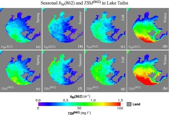
3.3. Seasonal Variability of the NIR-Based TSM in Lake Taihu

As demonstrated in Wang et al. [40,41] with MODIS water property products in Lake Taihu, Lake Taihu experienced significant spatial and temporal variations in terms of the water optical, biological, and biogeochemical properties. Using VIIRS-SNPP five-year observations from 2012 to 2016, seasonal climatology images of nL_w(745) and nL_w(862) were also derived. Figure 5 shows the seasonal climatology images of nL_w(745) (Figure 5a–d) and nL_w(862) (Figure 5e–h) for the season of boreal spring (March–May), summer (June–August), autumn (September–November), and winter (December–February). For each pixel, all of the corresponding valid nL_w(λ) spectra derived from VIIRS observations for that season (i.e., spring, summer, fall, and winter) between 2012 and 2016 are selected, and the median value of the valid nL_w(λ) at that pixel is calculated as the climatology nL_w(λ) value for that season. Similarly, the seasonal climatology of b_bp(λ) and TSM^(λ) is also computed. In general, nL_w(745) and nL_w(862) in Lake Taihu show significant seasonal variability with enhanced nL_w(745) and nL_w(862) in the winter season, and depressed nL_w(745) and nL_w(862) in the summer season. As an example, nL_w(745) actually reaches over ~3 mW cm⁻² μm⁻¹ sr⁻¹ in the Southern Lake Taihu in the winter, while its value is only ~1 mW cm⁻² μm⁻¹ sr⁻¹ in the summer. However, in Meiliang Bay part of Northern Lake Taihu (see the location in Figure 1), nL_w(745) peaks in the summer and autumn, while low nL_w(745) is observed in the winter season.

The spatial variability of nL_w(745) and nL_w(862) in each season is also significant. In winter, nL_w(745) and nL_w(862) in the southern lake region are ~3–4 times larger than those in the Northern Lake Taihu. However, in summer the nL_w(745) and nL_w(862) are higher in Northern Lake Taihu than in Southern Lake Taihu. It is also noted that both the temporal and spatial variations of VIIRS nL_w(745) and nL_w(862) are consistent with the nL_w(859) and K_d(490) derived from MODIS-Aqua observations in Lake Taihu [40,41].

We also derive VIIRS seasonal b_bp(862) and TSM⁽⁸⁶²⁾ from nL_w(862) in Lake Taihu. Figure 6 shows b_bp(862) (Figure 6a–d) and TSM⁽⁸⁶²⁾ (Figure 6e–h) in the spring, summer, autumn, and winter seasons. As expected, similar results are obtained for b_bp(745) and TSM⁽⁷⁴⁵⁾ (not shown). Due to the intrinsic relationship between b_bp(λ) and nL_w(λ) in the NIR wavelengths, the spatial and seasonal changes of the b_bp(745) and b_bp(862) follow the changes of nL_w(745) and nL_w(862) as expected. Significantly higher b_bp(862) and TSM⁽⁸⁶²⁾ can be found in Southern Lake Taihu in winter (Figure 6d,h). In contrast, b_bp(862) and TSM⁽⁸⁶²⁾ are actually lower in Southern Lake Taihu than those in Northern Lake Taihu in the summer (Figure 6b,f). The peaks in b_bp(862) and TSM⁽⁸⁶²⁾ during the winter might be attributed to the enhanced sediment suspension due to strong monsoon winds [24].

The particle backscattering coefficient b_bp(λ) is spectrally correlated and generally can be modeled as a function of b_bp(λ) at another wavelength [65], i.e.,

$$b_{bp}(\lambda )=b_{bp}({\lambda }_0){\left(\frac{{\lambda }_0}{\lambda }\right)}^{\eta }$$

(8)

Examination of b_bp(862) and b_bp(745) (not shown here) shows that they are almost identical in terms of both spatial pattern and magnitude in the winter. This suggests that the value of power law slope, η, is close to 0. On the other hand, b_bp(745) is higher than b_bp(862) in the spring, summer, and autumn, suggesting that the value of power law slope, η, is positive. Since η is related to the suspended sediment properties, such as the particle size distribution, particle compositions, etc., the seasonal change of the power law slope, η, might have further biological and biogeochemical implications for Lake Taihu.

Using Equations (6) and (7), seasonal variability of TSM concentration in Lake Taihu is also derived. Figure 6 shows TSM concentration TSM⁽⁸⁶²⁾ (Figure 6e–h) derived from b_bp(862) in the four seasons. In the winter season, TSM concentration can reach over ~100 mg L⁻¹ in Southern Lake Taihu, while low TSM concentration of ~10 mg L⁻¹ is observed in Meiliang Bay, part of Northern Lake Taihu. Even though the formulae for TSM⁽⁷⁴⁵⁾ and TSM⁽⁸⁶²⁾ are different (Equations (6) and (7)), TSM⁽⁸⁶²⁾ and TSM⁽⁷⁴⁵⁾ (not shown here) are indeed similar for all four seasons in terms of the TSM values and their spatial patterns.

It is also noted that the seasonal variation of b_bp(λ) and TSM in Meiliang Bay is different from the other regions with pronounced b_bp(λ) and TSM in summer, and autumn seasons (Figure 6), while peaks of b_bp(λ) and TSM occurred in the winter season for the other parts of the lake. This might be attributed to the frequent occurrence of floating blue algae blooms in the three seasons in Meiliang Bay, which can consequently enhance the nL_w(745) and nL_w(862), and lead to possible overestimation of the TSM concentrations in the bay.

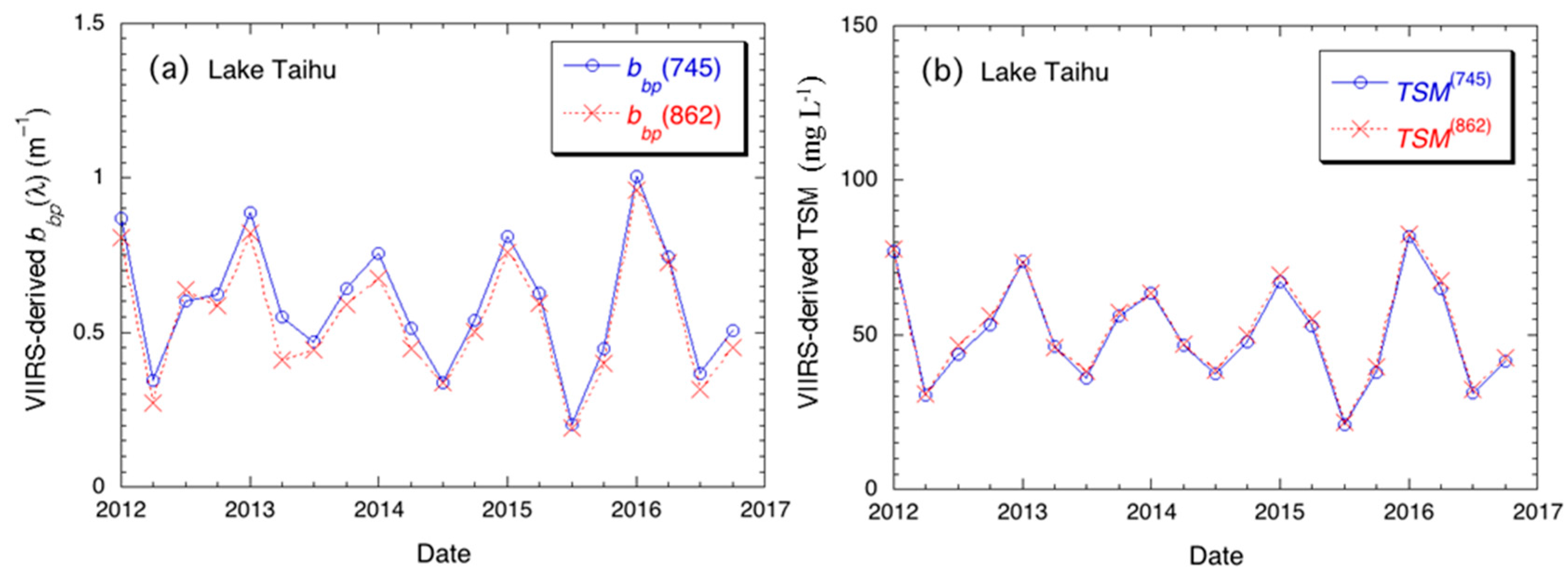
3.4. Interannual Variability of VIIRS NIR-Based Products in Lake Taihu

Previous studies show that the interannual variability of environmental parameters, such as Chl-a, K_d(490), and primary production in Lake Taihu can be significant [40,47]. Figure 7 shows the composite images of b_bp(862) from 2012 to 2016. Even though those spatial patterns of b_bp(862) between 2012 and 2016 are similar to each other, interannual variability of the b_bp(862) is also remarkable. In Meiliang Bay and Gonghu Bay, low b_bp(862) were observed in 2014 and 2015 in comparison with the other years. In 2014 and 2015, the mean b_bp(862) in Meiliang Bay was about 0.3 m⁻¹, while it reached over ~0.4 m⁻¹ in the other years. Figure 7f–j show the corresponding TSM⁽⁸⁶²⁾ in 2012–2016. In general, the spatial distributions of TSM⁽⁸⁶²⁾ are similar to the spatial patterns of b_bp(862) in each year. Enhanced TSM⁽⁸⁶²⁾ over 100 mg/L was observed in southern Lake Taihu in the composite image of TSM⁽⁸⁶²⁾ in 2014. In terms of TSM⁽⁸⁶²⁾ for the entire Lake Taihu, 2014 was the least turbid year. In addition to b_bp(862) and TSM⁽⁸⁶²⁾ between 2012 and 2016, b_bp(745) and TSM⁽⁷⁴⁵⁾ (not shown here) show similar results as b_bp(862) and TSM⁽⁸⁶²⁾ in these years.

Figure 8 shows the interannual variability of the b_bp(λ) and TSM concentration for the entire Lake Taihu (Figure 8a,b). For the all of Lake Taihu, the average TSM concentration between 2012 and 2016 is ~41 mg L⁻¹ with TSM ranging between ~20–30 mg L⁻¹ in the summer and ~60–80 mg L⁻¹ in the winter, respectively. Highest b_bp(λ) and TSM concentrations occurred in the 2015–2016 winter with b_bp(λ) reaching over ~1.0 m⁻¹ and TSM concentrations over ~80 mg L⁻¹. TSM⁽⁷⁴⁵⁾ and TSM⁽⁸⁶²⁾ are indeed close to each other between 2012 and 2016. This further suggests that both TSM algorithms can be used to quantitatively evaluate the long-term TSM variations in Lake Taihu.

It is also noted that the TSM⁽⁷⁴⁵⁾ and TSM⁽⁸⁶²⁾ algorithms are both developed from the in situ TSM concentration, nL_w(745), and nL_w(862). Negligible differences between the TSM⁽⁷⁴⁵⁾ and TSM⁽⁸⁶²⁾ algorithms provides further evidence that VIIRS nL_w(745) and nL_w(862) derived using the SWIR-based atmospheric correction algorithm in Lake Taihu are reasonably accurate and comparable to the in-situ nL_w(λ) measurements. In combination with the negligible difference between TSM⁽⁷⁴⁵⁾ and TSM⁽⁸⁶²), it is also shown that both TSM⁽⁷⁴⁵⁾ and TSM⁽⁸⁶²⁾ can be confidently used to monitor, characterize, and quantify the TSM variation in Lake Taihu.

4. Discussion

In a recent study [33], we have shown that for highly turbid waters b_bp(λ) in the NIR wavelengths can be derived analytically due to strong water absorption in the NIR wavelengths. In fact, b_bp(λ) in visible wavelengths can also be derived with b_bp(λ) in the NIR wavelengths. Using the International Ocean Color Coordinating Group (IOCCG) IOP dataset [65], it has been shown that this approach can derive accurate backscattering coefficients b_bp(λ) in the visible and NIR wavelengths. Since there are no simultaneous b_bp(λ) measurements in the in situ dataset in this study, the accuracy of b_bp(745) and b_bp(862) derived from in situ nL_w(745) and nL_w(862) cannot be evaluated directly. Examination of the in situ a_ph(λ) and a_cdom(λ) confirms that a_w(λ) values at VIIRS 745 and 862 nm bands are generally two orders higher than the in situ a_ph(λ) and a_cdom(λ) in these two NIR bands. This provides evidence that the analytical Equations (1)–(5) are valid in turbid waters, such as Lake Taihu for deriving reasonable b_bp(745) and b_bp(862) values from VIIRS-measured nL_w(745) and nL_w(862).

In this study, we demonstrated that b_bp(745) and b_bp(862) can be used to compute TSM concentrations in Lake Taihu with good accuracy. Using the coincident in situ TSM measurements and VIIRS-derived TSM⁽⁷⁴⁵⁾ and TSM⁽⁸⁶²⁾, we further validate the VIIRS TSM retrieval algorithms in Lake Taihu. Previous studies have already shown that the SWIR-based atmospheric correction with MODIS can be used to drive nL_w(λ) spectra with good accuracy in Lake Taihu [40,41], and the VIIRS sensor is well characterized and calibrated for all of the bands from the visible to SWIR wavelengths [55,70]. This shows that VIIRS-derived nL_w(λ) spectra in Lake Taihu are reasonably accurate and can be used to produce other biogeochemical products, such as the TSM concentration. Similar approaches and procedures can be applied to develop the TSM algorithm for other sensors, such as MODIS-Aqua and other coastal and inland waters, if the in situ optical and TSM measurements are available. On the other hand, b_bp(745) and b_bp(862) in Lake Taihu can be related to TSM, which are eventually associated with the TSM bio-physical properties such as particle composition, mineral type, particle size distributions, etc., in addition to TSM concentration. Since these properties are stable over time in Lake Taihu, the TSM algorithms in Equations (6) and (7) can be safely applied to VIIRS observations to monitor, characterize, and quantify TSM variability in Lake Taihu.

In addition to developing a regional TSM algorithm for Lake Taihu, the main purpose of this study is to demonstrate the usefulness of the NIR IOP b_bp(745) and b_bp(862) for developing algorithms for other biological and biogeochemical products over turbid coastal and inland waters. The intrinsic relationships between nL_w(λ) or b_bp(λ) in the NIR wavelengths and TSM concentration imply that the formula for TSM as shown in Equations (6) and (7) for Lake Taihu should be reasonably accurate if nL_w(λ) spectral shapes in the NIR wavelengths in other coastal and inland waters are similar to those in Lake Taihu. In fact, Shi and Wang (2014) [33] examined the ocean reflectance spectra in different regions in the Bohai Sea, Yellow Sea, and East China Sea from MODIS-Aqua observations. The NIR nL_w(748) and nL_w(869) show similar relationships for the Lake Taihu, Hangzhou Bay, and Yangtze River Estuary. The scatter plots of nL_w(748) and nL_w(869) in Lake Taihu, Hangzhou Bay, and Yangtze River Estuary generally overlap with each other in the range of 0–4 mW cm⁻² μm⁻¹ sr⁻¹ for nL_w(748), and the slopes of nL_w(748)/nL_w(869) are similar in these three regions. In comparison, the spectral shapes in these three regions are virtually different from those in the Yellow River Estuary and the Subei Shoal. In fact, waters of these three regions have the same sediment source from the Yangtze River [71]. This indicates that the TSM algorithms from this study can also be applied across these regions. From a broad global perspective, these two NIR-based TSM algorithms can be applied to regions where VIIRS nL_w(745) and nL_w(862) have a similar relationship to that in Lake Taihu in order to derive reasonably good TSM products.

Even though other efforts exist to derive the TSM concentrations from satellite observations in the region [21,23,72], there are some limitations in these algorithms in comparison with the NIR-based TSM algorithm. Particularly, nL_w(λ) at the green and red bands can become saturated in highly-turbid waters [24,33]. Thus, for highly-turbid waters, nL_w(λ) in the green and red wavelengths are not sensitive to the changes in the TSM concentrations. This suggests that the TSM algorithms based on nL_w(λ) in green and red bands have physical and optical limitations in deriving accurate TSM concentration in highly turbid waters. In comparison, the NIR-based algorithm is valid over a wide range of TSM concentrations and necessary for highly-turbid waters. It is also noted that these two TSM algorithms do not have limitations for high TSM situations. Unlike the nL_w(λ) in visible, nL_w(λ) at these two NIR bands cannot become saturated in any season in Lake Taihu. However, caution should be given for applying these two algorithms to clear open ocean waters due to the accuracy of the satellite-derived nL_w(λ) at NIR wavelengths. Particularly, the NIR nL_w(λ) over the global open ocean is usually negligible. Even though Equation (5) shows that TSM concentration computation from Equations (1)–(3) can be calculated without any bias at low TSM levels, uncertainty in satellite-derived NIR nL_w(λ) over the open ocean due to imperfect atmospheric correction can lead to errors in the retrieved TSM concentration.

5. Conclusions

In summary, we have demonstrated that TSM concentrations can be derived from the NIR-based nL_w(λ) in Lake Taihu from VIIRS measurements. Using TSM data derived from VIIRS observations, seasonal and interannual variability of the TSM concentration in Lake Taihu has been characterized and quantified. In comparison with other TSM algorithms, the approach reported here uses the TSM and the NIR IOP (i.e., b_bp(λ)) relationship. Through the NIR b_bp(λ) relationship, the TSM formulation can be expressed more clearly, in particular, how TSM should be related to water optics measurements. The NIR IOP-based TSM algorithm for turbid waters is more accurate, in particular, for waters with large TSM values, i.e., highly-turbid waters. From the global perspective, the IOP-based TSM algorithm has the potential to compute TSM concentration with good accuracy in the waters with similar NIR nL_w(λ) spectral shapes as those in Lake Taihu. Indeed, for highly-turbid coastal and inland waters, accurate TSM data can only be derived using satellite-measured optical information at the NIR wavelengths.

References

1. Wang, M.; Son, S.; Harding, L.W., Jr. Retrieval of diffuse attenuation coefficient in the Chesapeake Bay and turbid ocean regions for satellite ocean color applications. J. Geophys. Res. 2009, 114. [Google Scholar] [CrossRef]
2. Lee, Z.P.; Du, K.; Arnone, R. A model for the diffuse attenuation coefficient of downwelling irradiance. J. Geophys. Res. 2005, 110. [Google Scholar] [CrossRef]
3. Morel, A.; Huot, Y.; Gentili, B.; Werdell, P.J.; Hooker, S.B.; Franz, B.A. Examining the consistency of products derived from various ocean color sensors in open ocean (Case 1) waters in the perspective of a multi-sensor approach. Remote Sens. Environ. 2007, 111, 69–88. [Google Scholar] [CrossRef]
4. O’Reilly, J.E.; Maritorena, S.; Mitchell, B.G.; Siegel, D.A.; Carder, K.L.; Garver, S.A.; Kahru, M.; McClain, C.R. Ocean color chlorophyll algorithms for SeaWiFS. J. Geophys. Res. 1998, 103, 24937–24953. [Google Scholar] [CrossRef]
5. Hu, C.; Lee, Z.; Franz, B.A. Chlorophyll a algorithms for oligotrophic oceans: A novel approach based on three-band reflectance difference. J. Geophys. Res. 2012, 117. [Google Scholar] [CrossRef]
6. Wang, M.; Son, S. VIIRS-derived chlorophyll-a using the ocean color index method. Remote Sens. Environ. 2016, 182, 141–149. [Google Scholar] [CrossRef]
7. Behrenfeld, M.J.; Falkowski, P.G. Photosynthetic rates derived from satellite-based chlorophyll concentration. Limnol. Oceanogr. 1997, 42, 1–20. [Google Scholar] [CrossRef]
8. Antoine, D.; Morel, A. Oceanic primary production 1. Adaptation of a spectral light photosynthesis model in view of application to satellite chlorophyll observations. Glob. Biogeochem. Cycles 1996, 10, 43–55. [Google Scholar] [CrossRef]
9. Shi, W.; Wang, M. Satellite observations of flood-driven Mississippi River plume in the spring of 2008. Geophys. Res. Lett. 2009, 36. [Google Scholar] [CrossRef]
10. Mulder, T.; Syvitski, J.P.M. Turbidity currents generated at river mouths during exceptional discharges to the world oceans. J. Geol. 1995, 103, 285–299. [Google Scholar] [CrossRef]
11. Harden, C.P. Land use, soil erosion, and reservoir sedimentation in an Andean Drainage Basin in Ecuador. Mountain Res. Dev. 1993, 13, 177–184. [Google Scholar] [CrossRef]
12. Hu, C.; Muller-Karger, F.E. Response of sea surface properties to Hurricane Dennis in the eastern Gulf of Mexico. Geophys. Res. Lett. 2007, 34. [Google Scholar] [CrossRef]
13. Shi, W.; Wang, M. Observations of a Hurricane Katrina-induced phytoplankton bloom in the Gulf of Mexico. Geophys. Res. Lett. 2007, 34. [Google Scholar] [CrossRef]
14. Shi, W.; Wang, M. Three-dimensional observations from MODIS and CALIPSO for ocean responses to cyclone Nargis in the Gulf of Martaban. Geophys. Res. Lett. 2008, 35. [Google Scholar] [CrossRef]
15. Shi, W.; Wang, M.; Jiang, L. Spring-neap tidal effects on satellite ocean color observations in the Bohai Sea, Yellow Sea, and East China Sea. J. Geophys. Res. 2011, 116. [Google Scholar] [CrossRef]
16. Shi, W.; Wang, M.; Jiang, L. Tidal effects on ecosystem variability in the Chesapeake Bay from MODIS-Aqua. Remote Sens. Environ. 2013, 138, 65–76. [Google Scholar] [CrossRef]
17. Miller, R.L.; McKee, B. Using MODIS Terra 250 m imagery to map concentrations of total suspended matter in coastal waters. Remote Sens. Environ. 2004, 93, 259–266. [Google Scholar] [CrossRef]
18. Doxaran, D.; Froidefond, J.M.; Lavender, S.; Castaing, P. Spectral signature of highly turbid waters—Application with SPOT data to quantify suspended particulate matter concentrations. Remote Sens. Environ. 2002, 81, 149–161. [Google Scholar] [CrossRef]
19. Son, S.; Wang, M. Water properties in Chesapeake Bay from MODIS-Aqua measurements. Remote Sens. Environ. 2012, 123, 163–174. [Google Scholar] [CrossRef]
20. Tassan, S. An improved in-water algorithm for the determination of chlorophyll and suspended sediment concentration from Thematic Mapper data in coastal waters. Int. J. Remote Sens. 1993, 14, 1221–1229. [Google Scholar] [CrossRef]
21. Zhang, M.; Tang, J.; Dong, Q.; Song, Q.; Ding, J. Retrieval of total suspended matter concentration in the Yellow and East China Seas from MODIS imagery. Remote Sens. Environ. 2010, 114, 392–403. [Google Scholar] [CrossRef]
22. Mao, Z.H.; Chen, J.Y.; Pan, D.L.; Tao, B.Y.; Zhu, Q.K. A regional remote sensing algorithm for total suspended matter in the East China Sea. Remote Sens. Environ. 2012, 124, 819–831. [Google Scholar] [CrossRef]
23. Chen, J.; Quan, W.T.; Cui, T.W.; Song, Q.J. Estimation of total suspended matter concentration from MODIS data using a neural network model in the China eastern coastal zone. Estuar. Coast. Shelf Sci. 2015, 155, 104–113. [Google Scholar] [CrossRef]
24. Shi, W.; Wang, M. Satellite views of the Bohai Sea, Yellow Sea, and East China Sea. Prog. Oceanogr. 2012, 104, 30–45. [Google Scholar] [CrossRef]
25. Wang, M.; Shi, W. Estimation of ocean contribution at the MODIS near-infrared wavelengths along the east coast of the US: Two case studies. Geophys. Res. Lett. 2005, 32. [Google Scholar] [CrossRef]
26. Wang, M.; Tang, J.; Shi, W. MODIS-derived ocean color products along the China east coastal region. Geophys. Res. Lett. 2007, 34. [Google Scholar] [CrossRef]
27. Gitelson, A.A.; Schalles, J.F.; Hladik, C.M. Remote chlorophyll-a retrieval in turbid, productive estuaries: Chesapeake Bay case study. Remote Sens. Environ. 2007, 109, 464–472. [Google Scholar] [CrossRef]
28. Gordon, H.R.; Brown, O.B.; Evans, R.H.; Brown, J.W.; Smith, R.C.; Baker, K.S.; Clark, D.K. A Semianalytic Radiance Model of Ocean Color. J. Geophys. Res. Atmos 1988, 93, 10909–10924. [Google Scholar] [CrossRef]
29. Garver, S.A.; Siegel, D.A. Inherent optical property inversion of ocean color spectra and its biogeochemical interpretation: 1. Time series from the Sargasso Sea. J. Geophys. Res. 1997, 102, 18607–18625. [Google Scholar] [CrossRef]
30. Lee, Z.P.; Carder, K.L.; Arnone, R.A. Deriving inherent optical properties from water color: A multiple quasi-analytical algorithm for optically deep waters. Appl. Opt. 2002, 41, 5755–5772. [Google Scholar] [CrossRef] [PubMed]
31. Werdell, P.J.; Franz, B.A.; Bailey, S.W.; Feldman, G.C.; Boss, E.; Brando, V.E.; Dowell, M.; Hirata, T.; Lavender, S.J.; Lee, Z.P.; et al. Generalized ocean color inversion model for retrieving marine inherent optical properties. Appl. Opt. 2013, 52, 2019–2037. [Google Scholar] [CrossRef] [PubMed]
32. Shi, W.; Wang, M. An assessment of the black ocean pixel assumption for MODIS SWIR bands. Remote Sens. Environ. 2009, 113, 1587–1597. [Google Scholar] [CrossRef]
33. Shi, W.; Wang, M. Ocean reflectance spectra at the red, near-infrared, and shortwave infrared from highly turbid waters: A study in the Bohai Sea, Yellow Sea, and East China Sea. Limnol. Oceanogr. 2014, 59, 427–444. [Google Scholar] [CrossRef]
34. Le, C.F.; Li, Y.M.; Zha, Y.; Sun, D.Y.; Yin, B. Validation of a Quasi-Analytical Algorithm for highly turbid eutrophic water of Meiliang Bay in Taihu Lake, China. IEEE Trans. Geosci. Remote Sens. 2009, 47, 2492–2500. [Google Scholar]
35. Huang, J.; Chen, L.Q.; Chen, X.L.; Tian, L.Q.; Feng, L.; Yesou, H.; Li, F.F. Modification and validation of a quasi-analytical algorithm for inherent optical properties in the turbid waters of Poyang Lake, China. J. Appl. Remote Sens. 2014, 8. [Google Scholar] [CrossRef]
36. Qing, S.; Tang, J.W.; Cui, T.W.; Zhang, J. Retrieval of inherent optical properties of the Yellow Sea and East China Sea using a quasi-analytical algorithm. Chin. J. Oceanol. Limn. 2011, 29, 33–45. [Google Scholar] [CrossRef]
37. Hale, G.M.; Querry, M.R. Optical constants of water in the 200 nm to 200µm wavelength region. Appl. Opt. 1973, 12, 555–563. [Google Scholar] [CrossRef] [PubMed]
38. Kou, L.; Labrie, D.; Chylek, P. Refractive indices of water and ice in the 0.65–2.5 µm spectral range. Appl. Opt. 1993, 32, 3531–3540. [Google Scholar] [CrossRef] [PubMed]
39. Wang, M. Remote sensing of the ocean contributions from ultraviolet to near-infrared using the shortwave infrared bands: Simulations. Appl. Opt. 2007, 46, 1535–1547. [Google Scholar] [CrossRef] [PubMed]
40. Wang, M.; Shi, W.; Tang, J.W. Water property monitoring and assessment for China’s inland Lake Taihu from MODIS-Aqua measurements. Remote Sens. Environ. 2011, 115, 841–854. [Google Scholar] [CrossRef]
41. Wang, M.; Son, S.; Zhang, Y.; Shi, W. Remote sensing of water optical property for China’s inland Lake Taihu using the SWIR atmospheric correction with 1640 and 2130 nm bands. IEEE J. Sel. Top. Appl. Earth Obs. Remote Sens. 2013, 6, 2505–2516. [Google Scholar] [CrossRef]
42. Shi, K.; Zhang, Y.L.; Zhu, G.W.; Liu, X.H.; Zhou, Y.Q.; Xu, H.; Qin, B.Q.; Liu, G.; Li, Y.M. Long-term remote monitoring of total suspended matter concentration in Lake Taihu using 250 m MODIS-Aqua data. Remote Sens. Environ. 2015, 164, 43–56. [Google Scholar] [CrossRef]
43. Qin, B.; Xu, P.; Wu, Q.; Luo, L.; Zhang, Y. Environmental issues of Lake Taihu, China. Hydrobiologia 2007, 581, 3–14. [Google Scholar] [CrossRef]
44. Qin, B.; Zhu, G.; Gao, G.; Zhang, Y.; Li, W.; Paerl, H.W.; Carmichael, W.W. A drinking water crisis in Lake Taihu, China: Linkage to climatic variability and lake management. Environ. Manag. 2010, 45, 105–112. [Google Scholar] [CrossRef] [PubMed]
45. Zhu, M.; Zhu, G.; Zhao, L.; Yao, X.; Zhang, Y.; Gao, G.; Qin, B. Influence of algal bloom degradation on nutrient release at the sediment-water interface in Lake Taihu, China. Environ. Sci. Pollut. Res. 2013, 20, 1803–1811. [Google Scholar] [CrossRef] [PubMed]
46. Qin, B.; Gao, G.; Zhu, G.; Zhang, Y.; Song, Y.; Tang, X.; Xu, H.; Deng, J. Lake eutrophication and its ecosystem response. Chin. Sci. Bull. 2013, 58, 961–970. [Google Scholar] [CrossRef]
47. Zhang, Y.; Qin, B.; Liu, M. Temporal-spatial variations of chlorophyll a and primary production in Meiliang Bay, Lake Taihu, China. J. Plankton Res. 2007, 29, 707–719. [Google Scholar] [CrossRef]
48. Yao, X.; Zhang, Y.L.; Zhu, G.W.; Qin, B.Q.; Feng, L.Q.; Cai, L.L.; Gao, G.A. Resolving the variability of CDOM fluorescence to differentiate the sources and fate of DOM in Lake Taihu and its tributaries. Chemosphere 2011, 82, 145–155. [Google Scholar] [CrossRef] [PubMed]
49. Zhang, Y.L.; van Dijk, M.A.; Liu, M.L.; Zhu, G.W.; Qin, B.Q. The contribution of phytoplankton degradation to chromophoric dissolved organic matter (CDOM) in eutrophic shallow lakes: Field and experimental evidence. Water Res. 2009, 43, 4685–4697. [Google Scholar] [CrossRef] [PubMed]
50. Zhang, Y.; Feng, L.; Li, J.; Luo, L.; Yin, Y.; Liu, M.; Li, Y. Seasonal-spatial variation and remote sensing of phytoplankton absorption in Lake Taihu, a large eutrophic and shallow lake in China. J. Plankton Res. 2010, 32, 1023–1037. [Google Scholar] [CrossRef]
51. Zhang, Y.; Liu, X.; Yin, Y.; Zhang, M.; Qin, B. A simple optical model to estimate diffuse attenuation coefficient of photosynthetically active radiation in an extremely turbid lake from surface reflectance. Opt. Express 2012, 20, 20482–20493. [Google Scholar] [CrossRef] [PubMed]
52. Shi, W.; Wang, M. Ocean dynamics observed by VIIRS day/night band satellite observations. Remote Sens. 2018, 10, 76. [Google Scholar] [CrossRef]
53. Goldberg, M.D.; Kilcoyne, H.; Cikanek, H.; Mehta, A. Joint Polar Satellite System: The United States next generation civilian polar-orbiting environmental satellite system. J. Geophys. Res. Atmos. 2013, 118, 13463–13475. [Google Scholar] [CrossRef]
54. McClain, C.R. A decade of satellite ocean color observations. Ann. Rev. Mar. Sci. 2009, 1, 19–42. [Google Scholar] [CrossRef] [PubMed]
55. Wang, M.; Liu, X.; Tan, L.; Jiang, L.; Son, S.; Shi, W.; Rausch, K.; Voss, K. Impact of VIIRS SDR performance on ocean color products. J. Geophys. Res. Atmos. 2013, 118, 10347–10360. [Google Scholar] [CrossRef]
56. Wang, M.; Naik, P.; Son, S. Out-of-band effects of satellite ocean color sensors. Appl. Opt. 2016, 55, 2312–2323. [Google Scholar] [CrossRef] [PubMed]
57. Clark, D.K.; Gordon, H.R.; Voss, K.J.; Ge, Y.; Broenkow, W.; Trees, C. Validation of atmospheric correction over the ocean. J. Geophys. Res. 1997, 102, 17209–17217. [Google Scholar] [CrossRef]
58. Wang, M.; Shi, W.; Jiang, L.; Voss, K. NIR- and SWIR-based on-orbit vicarious calibrations for satellite ocean color sensors. Opt. Express 2016, 24, 20437–20453. [Google Scholar] [CrossRef] [PubMed]
59. International Ocean-Colour Coordinating Group (IOCCG). Atmospheric Correction for Remotely-Sensed Ocean-Colour Products; Wang, M., Ed.; Reports of International Ocean-Colour Coordinating Group, No. 10; IOCCG: Dartmouth, NS, Canada, 2010; p. 77. [Google Scholar]
60. Gordon, H.R.; Wang, M. Retrieval of water-leaving radiance and aerosol optical thickness over the oceans with SeaWiFS: A preliminary algorithm. Appl. Opt. 1994, 33, 443–452. [Google Scholar] [CrossRef] [PubMed]
61. Wang, M.; Shi, W. The NIR-SWIR combined atmospheric correction approach for MODIS ocean color data processing. Opt. Express 2007, 15, 15722–15733. [Google Scholar] [CrossRef] [PubMed]
62. Wang, M.; Son, S.; Shi, W. Evaluation of MODIS SWIR and NIR-SWIR atmospheric correction algorithms using SeaBASS data. Remote Sens. Environ. 2009, 113, 635–644. [Google Scholar] [CrossRef]
63. Lee, Z.P.; Carder, K.L.; Mobley, C.D.; Steward, R.G.; Patch, J.S. Hyperspectral remote sensing for shallow waters: 2. Deriving bottom depths and water properties by optimization. Appl. Opt. 1999, 38, 3831–3843. [Google Scholar] [CrossRef] [PubMed]
64. Babin, M.; Stramski, D. Light absorption by aquatic particles in the near-infrared spectral region. Limnol. Oceanogr. 2002, 47, 911–915. [Google Scholar] [CrossRef]
65. International Ocean-Colour Coordinating Group (IOCCG). Remote Sensing of Inherent Optical Properties: Fundamentals, Tests of Algorithms, and Applications; Lee, Z., Ed.; Reports of International Ocean-Colour Coordinating Group, No. 5; IOCCG: Dartmouth, NS, Canada, 2006; p. 125. [Google Scholar]
66. Stramski, D.; Babin, M.; Wozniak, S.B. Variations in the optical properties of terrigenous mineral-rich particulate matter suspended in seawater. Limnol. Oceanogr. 2007, 52, 2418–2433. [Google Scholar] [CrossRef]
67. Wozniak, S.B.; Stramski, D. Modeling the optical properties of mineral particles suspended in seawater and their influence on ocean reflectance and chlorophyll estimation from remote sensing algorithms. Appl. Opt. 2004, 43, 3489–3503. [Google Scholar] [CrossRef] [PubMed]
68. Shi, W.; Wang, M.H. Characterization of particle backscattering of global highly turbid waters from VIIRS ocean color observations. J. Geophys. Res. Oceans 2017, 122, 9255–9275. [Google Scholar] [CrossRef]
69. Gordon, H.R.; Morel, A. Remote Assessment of Ocean Color for Interpretation of Satellite Visible Imagery: A Review; Spring: New York, NY, USA, 1983. [Google Scholar]
70. Sun, J.; Wang, M. VIIRS reflective solar bands calibration progress and its impact on ocean color products. Remote Sens. 2016, 8, 194. [Google Scholar] [CrossRef]
71. Milliman, J.D.; Shen, H.T.; Yang, Z.S.; Mead, R.H. Transport and depositon of river sediment in the Changjiang estuary and adjacent continental shelf. Cont. Shelf Res. 1985, 4, 37–45. [Google Scholar] [CrossRef]
72. Zhou, W.; Wang, S.; Zhou, Y.; Troy, A. Mapping the concentrations of total suspended mater in Lake Taihu, China, using Landsat-5 TM data. Int. J. Remote Sens. 2006, 27, 1177–1191. [Google Scholar] [CrossRef]
Figure 1. Maps of China’s inland Lake Taihu. Locations of the in situ TSM measurements. Between 2012 and 2016 are marked as “×” in Lake Taihu.
Remotesensing 10 00333 g001
Figure 2. Scatter plots of in situ-derived bbp(λ) versus in situ TSM concentration in Lake Taihu for bbp(λ) at wavelengths of (a) 551 nm, (b) 671 nm, (c) 745 nm, and (d) 862 nm.
Remotesensing 10 00333 g002
Figure 3. Scatter plots for (a) bbp(745)-derived versus in situ-measured TSM, (b) bbp(862)-derived versus in situ-measured TSM, and (c) bbp(862)-derived versus bbp(745)-derived TSM.
Remotesensing 10 00333 g003
Figure 4. Scatter plots of (a) VIIRS bbp(745)-derived TSM(745) versus in situ-measured TSM and (b) VIIRS bbp(862)-derived TSM(862) versus in situ-measured TSM.
Remotesensing 10 00333 g004
Figure 5. Seasonal climatology nLw(745) images (ad) and nLw(862) images (eh) for spring, summer, autumn, and winter from VIIRS 2012–2016 measurements, respectively.
Remotesensing 10 00333 g005
Figure 6. Seasonal climatology bbp(862) images (ad) and TSM(862) images (eh) for spring, summer, autumn, and winter from VIIRS 2012–2016 measurements, respectively.
Remotesensing 10 00333 g006
Figure 7. VIIRS-derived yearly composite images of bbp(862) (ae) and TSM(862) (fj) in the corresponding years of 2012–2016.
Remotesensing 10 00333 g007
Figure 8. Variations of VIIRS-derived (a) bbp(745) and bbp(862), (b) TSM(745) and TSM(862) for the entirety of Lake Taihu.
Remotesensing 10 00333 g008