SatFog is an algorithm designed to detect fog presence in near-real time and thus gives indication on its temporal evolution. Based on threshold tests, SatFog relies uniquely on MSG-SEVIRI and no other ancillary data. SatFog uses the output of C-MACSP cloud detection algorithm and it classifies as low cloud or fog the nine HRV pixels contained in the narrowband pixel identified as low/middle clouds or clear sky by C-MACSP. SatFog works over land in daytime condition, i.e., when solar zenith angle is less than 85°. This because SatFog was developed to improve the estimation of solar energy power production, mainly available over land during daylight hours. The land mask has been derived from the GTOPO30 [
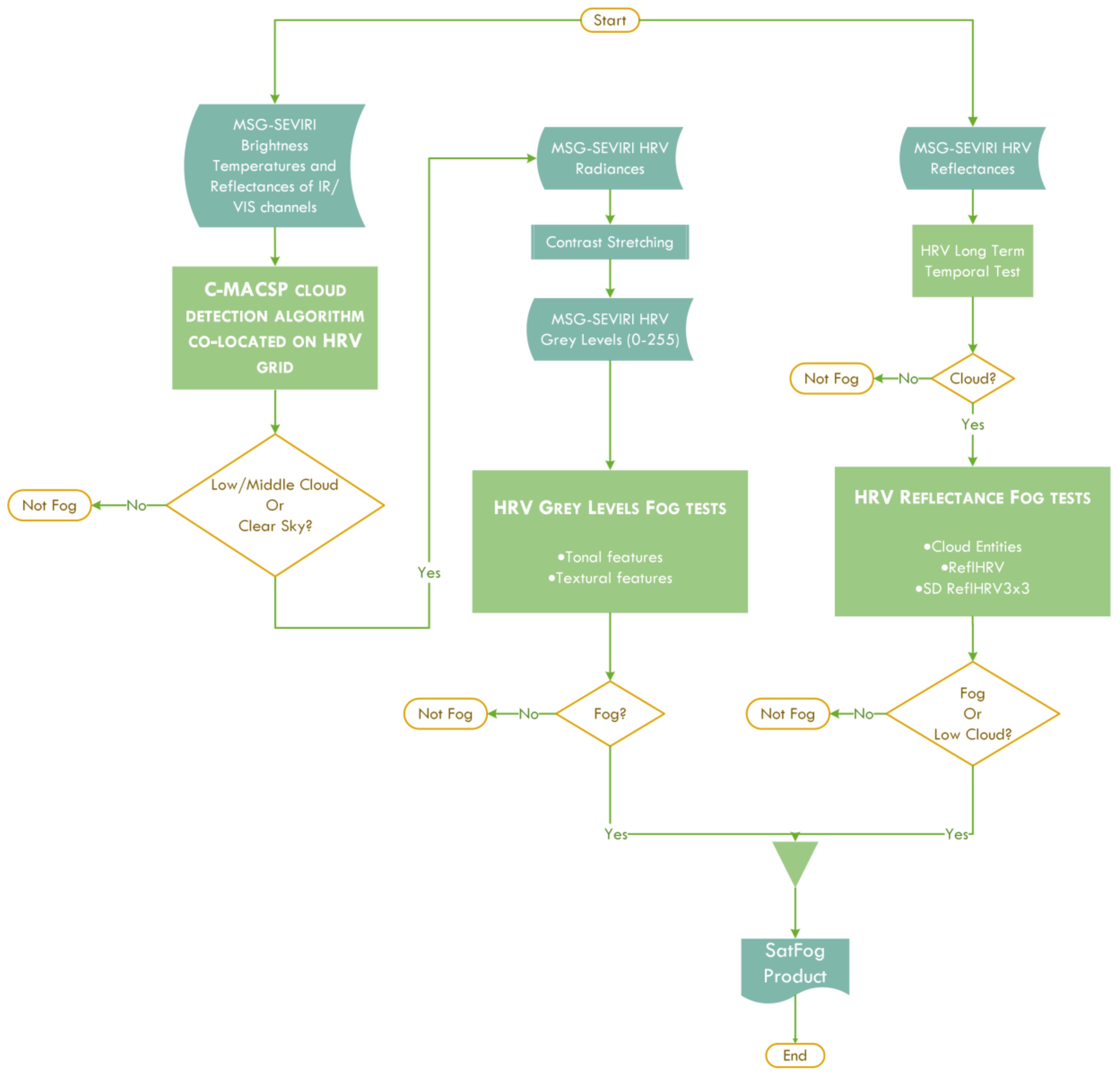
17] digital elevation model (DEM). GTOPO30 has a horizontal resolution of 30 arcsec, corresponding approximately to 1 km. The DEM grid has been upscaled at the spatial resolution of the HRV, by averaging the GTOPO30 values falling in each HRV pixel. DEM values greater than zero are selected for the land mask. SatFog algorithm is currently set up to run on a domain size of approximately 600 km (E-W) by 1200 km (N-S), covering the whole Italian peninsula. Here, the Po Valley and the Apennines and Alpine valleys are often affected by fog during autumn and spring, especially in the morning hours, when high-pressure stable condition and thermal inversion near the ground are present. SatFog aims at detecting this kind of fog events, characterized by very sharp boundaries and surrounded by clear sky pixels. SatFog does not take into account the pixels covered by snow/ice or by multi-layered clouds. Currently multi-layered clouds are not classified by C-MACSP. Only the highest cloud layer is classified in the pixel and it could be high thin/high thick cloud (in which case the pixel is automatically not considered by SatFog), or low/middle cloud (in which case the pixel is considered by SatFog). The block diagram giving an overview of SatFog is shown in
Figure 1.
The workflow is as follows. The algorithm calls C-MACSP to classify the cloud type at VIS/IR channel resolution and subsequently co-locates its output on HRV grid [
18] (left side of
Figure 1); henceforth, only low/middle clouds and cloud-free pixels are considered. It should be noticed that cloud-free pixels have to be included because the lower resolution of VIS/IR may hide smaller fog areas that could be otherwise detected by SatFog. In fact, it is possible that one or more of the nine HRV pixels co-located in a cloud-free C-MACSP pixel is not clear. The areas identified as cloud free or low/middle clouds by C-MACSP are further evaluated at HRV spatial resolution on the basis of HRV Grey Levels tests (central part of
Figure 1), in order to select those pixels characterized by the presence of fog. The HRV Grey Levels tests are applied to spatial and textural features; these are calculated by using the HRV radiances grey levels after a stretching contrast operation and the relative grey level co-occurrence matrix. Furthermore, HRV Reflectance Fog tests -specifically designed for HRV reflectances- have also been implemented (right side of
Figure 1): cloudy pixels are firstly selected by means of HRV Long Term Temporal Test and then linked in homogeneous cloud entities with the Cloud Entities test. Finally, the
ReflHRV and the SD
ReflHRV3×3 tests are applied to the reflectances and their standard deviations (calculated in 3-by-3 boxes) in order to identify among the cloud entities those areas characterized by the presence of fog or low clouds. The pixel classified as fog in all the aforementioned tests are finally flagged as fog and form the SatFog product. It is worth mentioning that suitable thresholds for HRV Grey Level Fog tests (central part of
Figure 1) and for HRV Reflectance Fog tests (right side of
Figure 1) were retrieved separately. In detail, a manually selected sample dataset was used to determine the thresholds for tonal and textural features tests, while the minimum HRV reflectance over the previous 10 days is used to determine the thresholds for HRV reflectance tests. Both classes of thresholds are dynamical because (i) the tonal and textural features are selected on the basis of the solar and satellite zenith angles and (ii) the HRV reflectance thresholds are calculated for each time slot. The HRV Grey Level Fog tests and the HRV Reflectance Fog tests are described in more detail in
Section 3.1 and
Section 3.3, respectively. The HRV reflectances used in the HRV Reflectance Fog tests are calculated according to the Bidirectional Reflectance Function (BDRF) for the SEVIRI warm channels formula (1)
where
3.1. HRV Grey Levels Fog Tests
This part includes tonal and textural tests used to classify pixels as fog, low cloud, or clear sky. Tonal and textural features (described in
Table 1) can be useful to identify objects in an image. Tonal features are strictly related to the image grey-level appearance and they describe the average tonal variations in a spectral band. Textural features give information about the spatial distribution of tonal variations in a spectral band. Moreover, it is important to select correctly the size of the area for evaluating tonal and textural features in order to prevent one feature from dominating over the other [
19]. In this study, a 3 × 3 box is chosen. We also considered the tonal and textural features determined in 5 × 5 box but their discriminating power is lower than that of the 3 × 3 box tonal and textural features. This is because a 5 × 5 (or higher) box provides information on a wider region, compared to the phenomenon we are interested. The range of textural and tonal characteristics values depends on the object that is observed: clear sky has got low values for contrast and entropy, while tonal features like maximum, minimum and mean strictly depend on spectral band. Generally, the high optically-thin clouds are characterized by entropy and ASM values lower than those characterizing high optically-thick clouds and higher than those related to low stratus or fog. This is due to the fact that generally high thick/thin clouds are characterized by a highly structured texture while the texture of low stratus and fog is smooth. Because of this, both low stratus and fog are characterized by entropy and ASM values lower than the values related to high thin/thick clouds and thus these features are not so useful for differentiating low stratus from fog. Conversely, on the basis of the Fisher criterion [
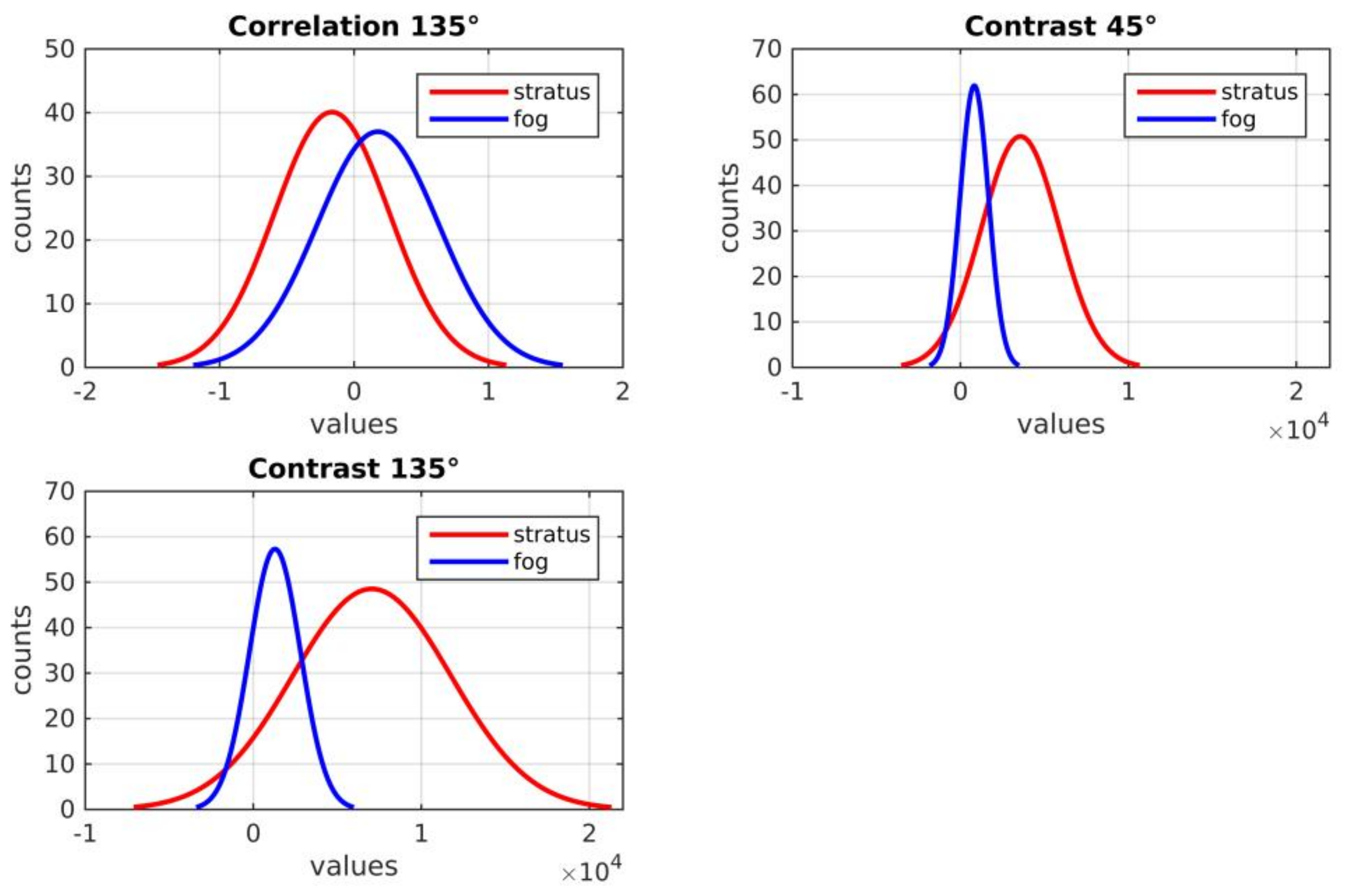
20,
21], the correlation and contrast at 135° and 45° have been chosen to discriminate low stratus from fog. This is supported by the distribution of correlation and contrast from the training set reported in
Figure 2. It can be noticed that the values of contrast at 45° and 135° are generally higher for stratus than for fog. The opposite happens, to a lesser extent, for correlation at 135°.
Starting from HRV radiances, grey levels quantized with 8 bits have been calculated. Grey levels (
) are the result of a linear contrast stretching operation (2) applied to the radiance intensity values.
where
is the HRV radiance of the pixel located at row x and column y in the HRV grid,
and
values are determined for the HRV study area at the time of interest and
is the number of all the possible grey levels (
).
After that, tonal and textural features have been extracted for the 3 × 3 HRV boxes. The tonal features considered here are the minimum, maximum, mean, standard deviation and median grey levels (the corresponding formulas are reported in
Table 1).
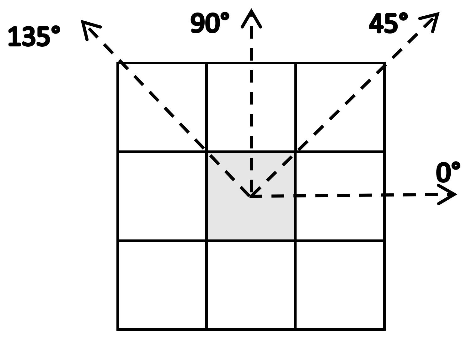
Following [
19], a Grey Level Co-occurrence Matrix (GLCM) has been created using neighbouring grey-tone (
Figure 3) in order to derive textural features. GLCM gives an indication of the spatial relationship of pixels and characterizes the texture of an image by calculating how often pairs of pixels with specific values and in an unambiguous spatial relationship occur in an image. Specifically, GLCM contains the normalized relative frequency,
, indicating how often two pixels with grey levels
and
separated by a distance
along the angle
occur within an image block. The separation distance
has been assumed
, while the angle
.
The textural features considered in this study are entropy, homogeneity, contrast, correlation and angular second moment calculated for the four directions (0, 45, 90, 135°) in the 3 × 3-pixel HRV boxes. The number of features has been reduced since not all proved to be useful for the classification. The criterion chosen for features reduction is the Fisher Distance
[
20,
21]:
where
is the mean and
is the standard deviation of the feature
for samples of class
.
quantifies the ability of the variable
to differentiate class
from class
. After the application of Fisher criterion, the selected features are min, max, mean, median grey levels, correlation 135° and contrast 45°, 135°. A positive fog test result is obtained when, considering the value of the
feature
, the pixel with coordinates
satisfies this condition
where
and
are, respectively, the minimum and the maximum thresholds for the Fog class. This procedure is applied to the other two classes too. In general, the thresholds used for the HRV Grey Levels Tests are calculated using the dataset of
Table 2. For each class of interest (Fog, Low cloud or Clear sky) and, respectively, for each feature described in
Table 1, the mean (
) and the standard deviation (
) have been calculated. Subsequently it has been chosen as
the difference between the mean and the standard deviation of the feature
for the class
while as
the sum of the mean and the standard deviation of the feature
for the same class. In detail:
Dataset Description
The threshold computation is a critical part of this algorithm. In this study, the data used for the threshold definition (
Table 2) have been manually selected on the basis of direct observations or the MSG-SEVIRI HRV images not used in algorithm evaluation (
Table 3). The test data set was built considering MSG-SEVIRI images collected in different areas at different times in daytime depending on the presence of fog, which was identified by direct knowledge from in-situ observations and visual inspection of RGB images. In detail, visual inspection has been used by further analysing the HRV pixels classified as low cloud by CMACSP. The HRV higher resolution is very useful in distinguishing stratus from fog. In fact, fog is characterized by sharper and more irregular edges than low stratus ones. Moreover, detecting valley fog is relatively simple because fog edges adapt themselves to the valley profile (or contours). These features have been observed not only in the HRV images but also in the HRV FOG RGB, consisting in a combination of the 1.6 µm channel on blue and of HRV channel on red and green [
22]. Since fog dissipates more quickly than stratus, the observation of the temporal behaviour of fog/stratus in HRV images was very useful to distinguish fog from low-stratus pixels. Although the careful visual inspection, the fact that passive satellite measurements do not provide direct information on cloud-base is a limitation in the correct detection of fog. By applying this procedure, both the dataset for the threshold determination and the test dataset were built. The SatFog HRV Grey Level tests thresholds are dynamically determined according to solar and satellite zenith and azimuth angles.
Table 2 and
Table 3 list the scenes used for the training of the HRV Grey Levels Fog tests and the evaluation, respectively. The accuracy (defined as the number R of the correctly classified samples, divided by the total number T of the samples,
) of the test dataset has been calculated for each sample. Accuracy values for the different classes (fog, low/middle clouds and clear sky) are reported in
Table 4. The number of samples used for the threshold determination for each class is respectively 509 (fog), 504 (low/middle clouds) and 509 (clear sky). The number of samples used for the accuracy calculation is respectively 270 (fog), 232 (low/middle clouds) and 406 (clear sky).
3.2. HRV Long Term Temporal Test
HRV Long Term Temporal Test (LTTT) has been developed to select only cloudy HRV pixel from SEVIRI HRV reflectances. The idea is to select cloudy pixels comparing the observation to a clear sky reference map built from previous 10-day observations at the same time and also to simulated clear sky reflectances. This test is composed by two steps: (i) clear sky reflectance is estimated as the minimum value of reflectance for each pixel in the previous 10 days (6); (ii) the difference between actual reflectance and the clear sky reflectance map (7) is compared with a threshold value. If the difference is larger than the threshold, the pixel is classified as cloudy (8). The threshold was estimated considering both simulated and measured clear sky datasets. The former provides a useful estimate of the threshold value variability around the minimum value calculated from the measured data [
23]. Using minimum composites in an operational context can lead to not very accurate results, that is why the suggested approach is the use of radiative transfer model simulations.
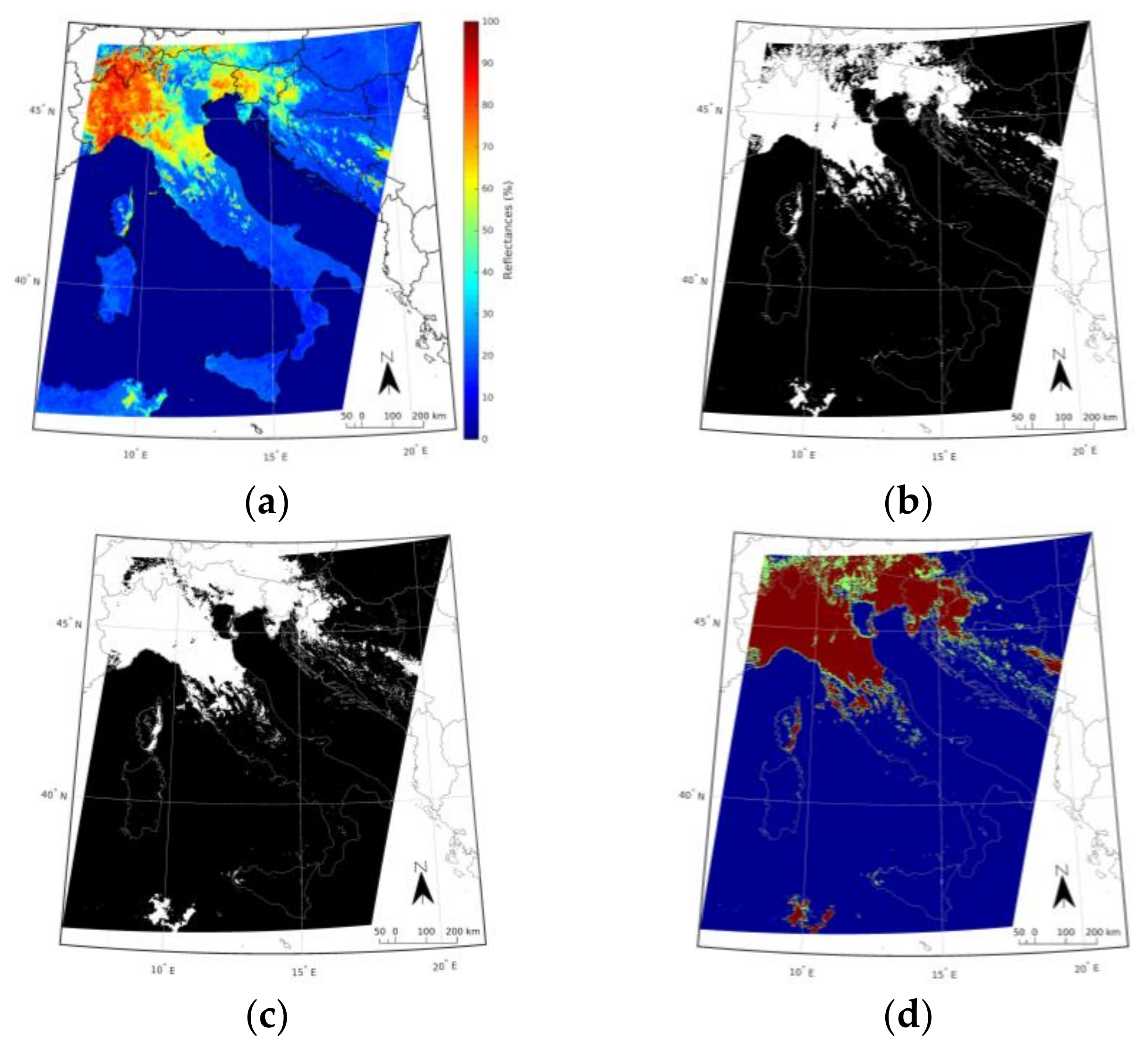
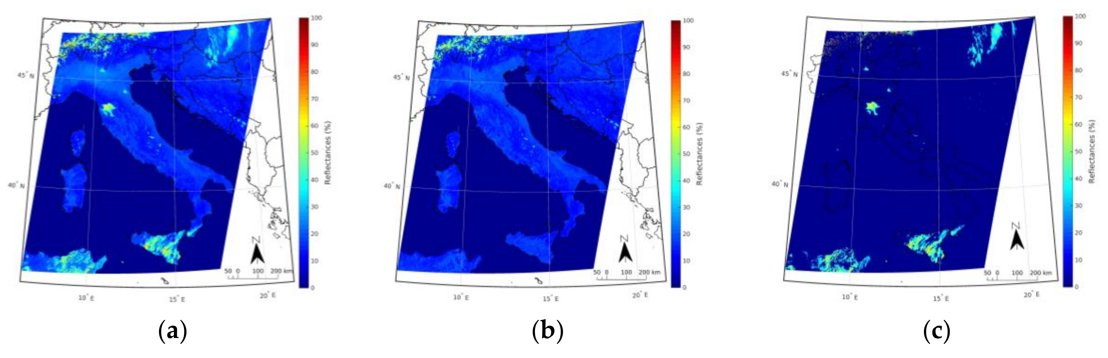
Figure 4 shows how the HRV LTTT product is obtained. The HRV reflectances are observed on 10.04.2017 at 07:45 UTC (
Figure 4a). In
Figure 4b the HRV clear sky reference map is reported.
Figure 4c shows the HRV LTTT cloudy areas land product. This approach permits to adapt the HRV LTTT product according to the temporal and spatial variability of the ground and of the atmosphere.
To highlight the plausibility of this approach a comparison with the MODIS cloud mask product (MOD35), re-gridded on the MSG-SEVIRI HRV grid is presented. In the literature, MODIS cloud retrieval products are widely used as terms for comparison to evaluate the performances of satellite cloud retrieval products [
24,
25,
26]. MOD35 is a daily, global Level 2 product generated at 1 km and 250 m (at nadir) spatial resolutions [
27]. The algorithm employs a series of visible and infrared threshold and consistency tests to specify confidence that an unobstructed view of the Earth’s surface is observed or not. The re-gridded mask is obtained using the minimum distance criterion between MSG-SEVIRI and MODIS pixel centres, considering that nominally the two products have the same spatial resolution (1 km). As shown in
Figure 5, the HRV LTTT produces a cloud mask in agreement with MOD35, though differences are evident in high thin cloud detection. Overall statistical scores are summarized in
Table 5.
3.3. HRV Reflectance Fog Tests
This series of tests include Cloud Entities,
ReflHRV and SD
ReflHRV3×3 tests. The aim is to locate fog or low stratus areas among the cloudy pixels selected by HRV LTTT. The Cloud Entities test is an object-oriented test. The object-oriented approach aims at the segmentation of the pixels into objects that are related by the same characteristics and permits to treat each object as a whole. In particular we are interested in the segmentation of the different cloud systems present into the domain. In fact, Cloud Entities test returns the connected component according to the 4 connected neighbours method (see
Figure 3) [
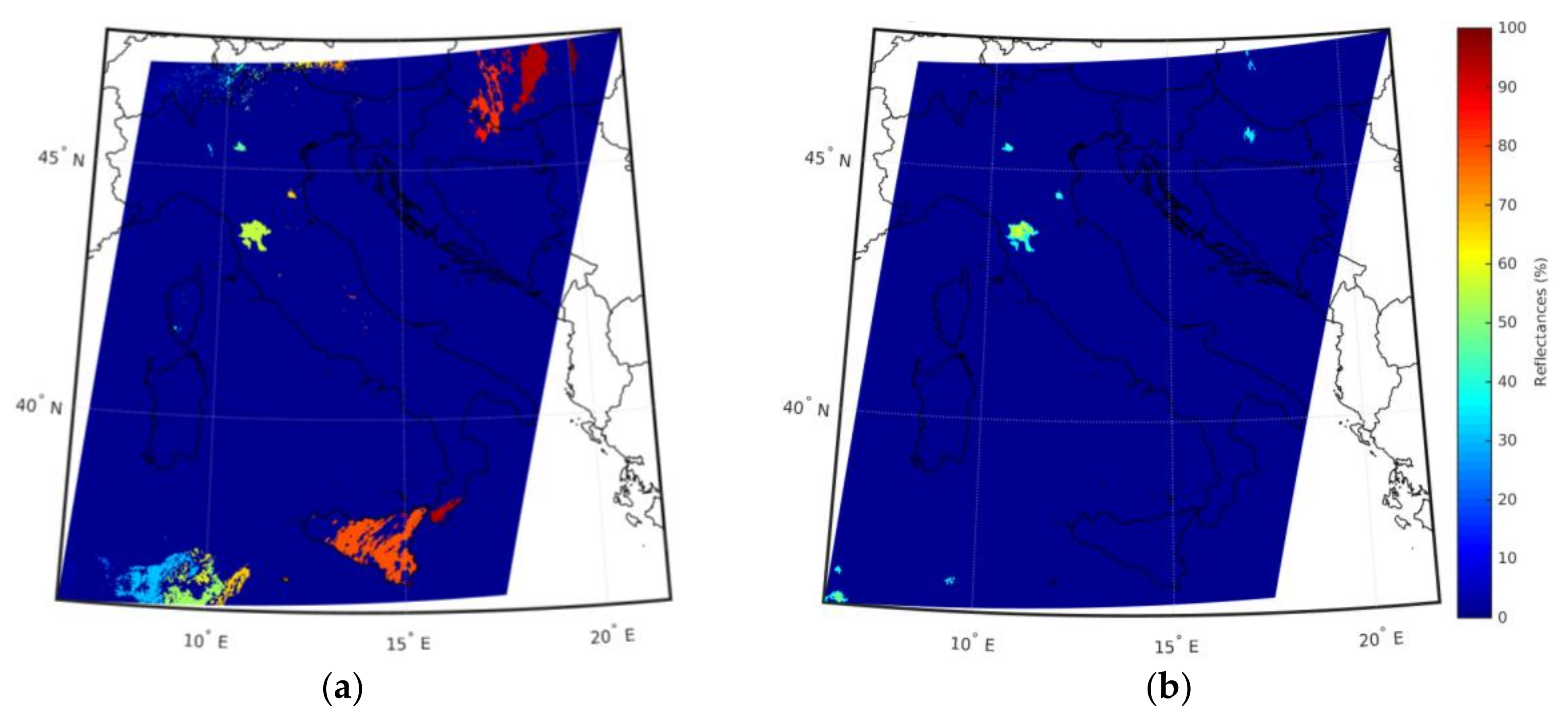
19]. Connected components are regions of adjacent pixels which share the same binary value. The Cloud Entities test provides a segmentation of cloudy areas in different cloud clusters, as shown in
Figure 6a in which each detected entity has been represented with a different colour. The
ReflHRV test and the SD
ReflHRV3×3 test are entity based threshold tests implemented to identify cloudy systems characterized by fog or very low clouds. The SD
ReflHRV3×3 thresholds are estimated using the reference database built with visually identified fog cases (see
Table 3). The
ReflHRV test aims at selecting those pixels included in minimum (
) and maximum (
) reflectance thresholds values. In detail:
where the
is the typical HRV reflectance in clear sky at a certain time calculated as the minimum HRV reflectance over the 10 days before at the same time of the day. This approach takes into account solar and satellite angle variations. The
is augmented by a pair of fixed values (
and
) to obtain the minimum and maximum thresholds values. The 0.15–0.30 range is assumed to account for variations in HRV reflectances due to meteorological variables such as water vapor and temperature.
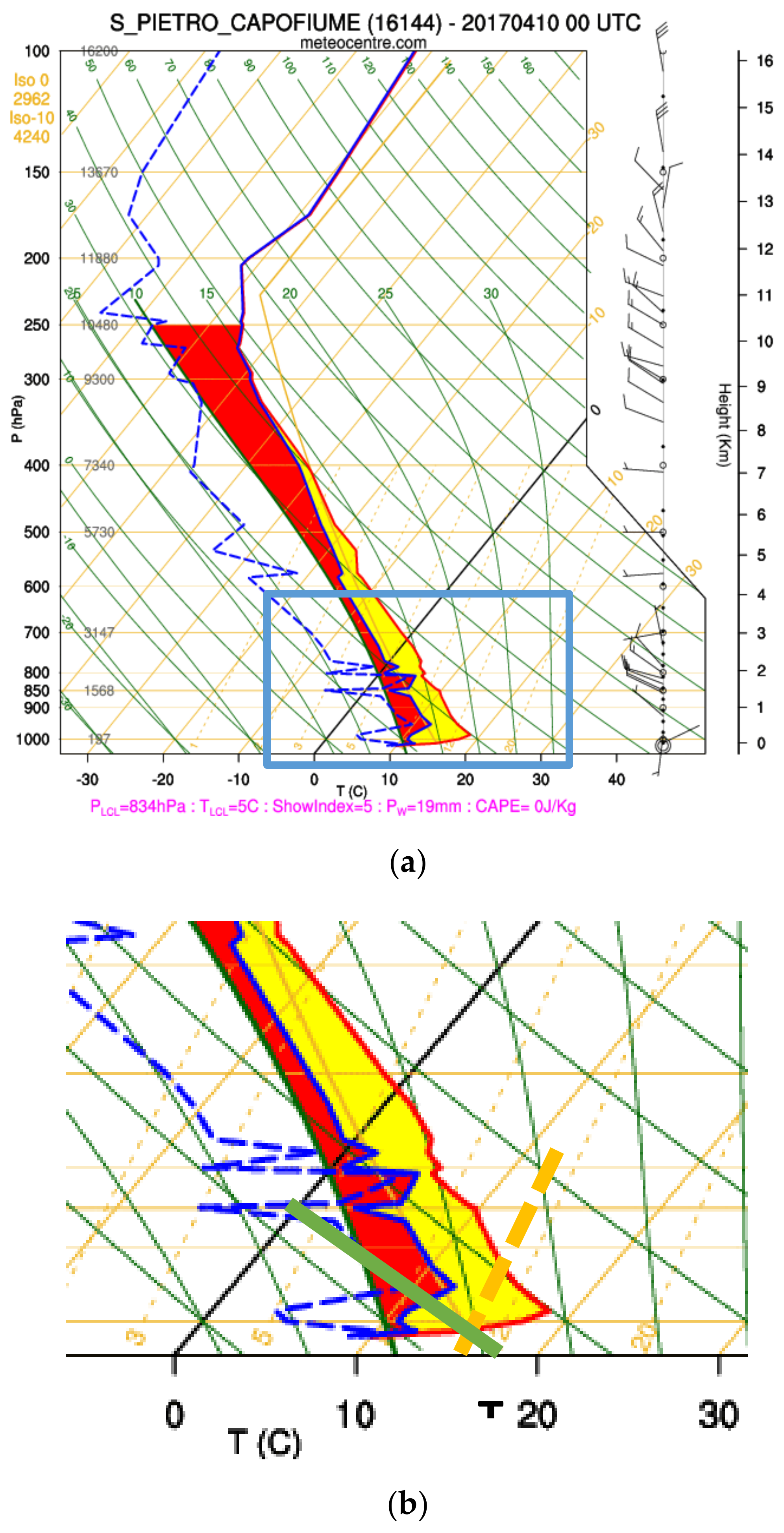
The presence of a temperature inversion at the fog top is one of the main features that lead to identify fog presence. A temperature inversion inhibits the vertical ascent of the water droplets forcing them to remain in the planetary boundary layer and so to form the fog or stratus layer. The altitude in which the inversion occurs is essential to discriminate fog from stratus. In detail, inversion altitudes lower than 500 m above the surface level should indicate fog presence while inversion altitudes higher than 500 m above the surface level should indicate the stratus presence [
11]. The evaluation of the spatial standard deviation of reflectance (SD
ReflHRV3×3, calculated in 3 × 3 HRV boxes centred on the pixel of interest) is very useful to discriminate clear sky from fog/low-stratus. By comparing the SD
ReflHRV3×3 calculated for the clear samples and the fog/low stratus samples of the training dataset, it results that the values of SD
ReflHRV3×3 associated to clear pixels are higher than that associated to fog/low stratus (SD
ReflHRV3×3 is 0.4 for clear sky while 0.1 for fog/low stratus). Our findings reveal that SD
ReflHRV3×3 values lower than dynamical thresholds, determined by taking into account the clear sky SD
ReflHRV3×3, indicate high probability of having fog/low stratus. This test has to be considered together with the other tests, as shown in the SatFog scheme in
Figure 1. An example of the final MSG-SEVIRI SatFog product is the map of fog covered areas shown in
Figure 6b.

 ,
, 


