Abstract
Focusing on the inverse synthetic aperture radar (ISAR) imaging of targets with complex motion, this paper proposes a modified version of the Fourier transform, called non-uniform rotation transform, to achieve cross-range compression. After translational motion compensation, the target’s complex motion is converted into non-uniform rotation. We define two variables—relative angular acceleration (RAA) and relative angular jerk (RAJ)—to describe the rotational nonuniformity. With the estimated RAA and RAJ, rotational nonuniformity compensation is carried out in the non-uniform rotation transform matrix, after which, a focused ISAR image can be obtained. Moreover, considering the possible deviation of RAA and RAJ, we design an optimization scheme to obtain the optimal RAA and RAJ according to the optimal quality of the ISAR image. Consequently, the ISAR imaging of targets with complex motion is converted into a parameter optimization problem in which a stable and clear ISAR image is guaranteed. Compared to precedent imaging methods, the new method achieves better imaging results with a reasonable computational cost. Experimental results verify the effectiveness and advantages of the proposed algorithm.
1. Introduction
Inverse synthetic aperture radar (ISAR) imaging is a key approach for the observation, surveillance, and recognition of space, aerial, and marine targets, with advantages of long working distance, high resolution, and all-day working capability [1,2,3,4]. The Fourier transform-based range-Doppler algorithm works well for imaging of targets with smooth motion, which has been widely used in ISAR imaging systems. In practice, however, the target’s motion is often complex, such as fluctuation of ships and high maneuvering of airplanes, which leads to the blurring of ISAR images obtained through the range-Doppler algorithm. It is believed that the complex motion of the target results in quadratic and even cubic phase terms in cross-range signals; thus, the conventional range-Doppler algorithm fails. To solve this problem, several approaches have been proposed, including slow time interpolation [5], joint time-frequency representation [5,6,7,8,9,10], parameter estimation of signal models [11,12,13,14,15], and super resolution methods [16,17,18,19,20,21].
The slow time interpolation method aims to obtain the uniform rotation angle through interpolation, after which conventional range-Doppler algorithm can be carried out. Given that translational motion has been compensated, the target’s complex motion can be regarded as non-uniform rotation. The idea of transforming non-uniform rotation into uniform rotation through interpolation is quite reasonable. However, this approach has some obvious demerits. First, obtaining prior information about the target’s rotational nonuniformity, which is necessary for interpolation, is troublesome. Though the multiple prominent points processing scheme [5] is an optional approach for non-uniform rotation estimation, it cannot guarantee accuracy owing to adverse factors such as noise interference and residual error of translational motion compensation. Second, the interpolated data are just an estimation of original data, and thus, the induced deviation is unavoidable. In summary, the interpolation method is effective to some degree, but there is scope for improvement.
Joint time-frequency representation methods are promising for motion compensation [5,6] and instantaneous Doppler frequency representation [7,8,9,10] in ISAR imaging. Chen et al. used the adaptive joint time-frequency projection technique to perform Doppler tracking of individual scatterers, where the translation motion error and rotational nonuniformity were compensated using the multiple prominent points processing scheme. Some researchers have also employed the joint time-frequency representation methods to obtain the range-instantaneous-Doppler (RID) image of the target. Since the instantaneous Doppler frequency of a scatterer is proportional to its azimuth position, the RID image has the capability of distinguishing scatterers in the cross-range direction. However, numerous scatterers are usually located in the same range cell, so cross-range signals are multi-component and nonstationary. In the field of signal processing, the time-frequency representation of multi-component and nonstationary signals faces problems of cross-term interference, heavy computation load and resolution loss [22]. Consequently, the quality of RID image is usually unsatisfactory and unstable.
Researchers have also proposed imaging algorithms based on parameter estimation of signal models [11,12]. Owing to the target’s equivalent non-uniform rotation, each scatterer causes a polynomial phase signal (PPS) such as a linear frequency-modulated (LFM) signal or cubic phase function (CPF) signal in the cross-range direction. Zheng et al. estimated the parameter of each PPS component, and then compensated the high-order phase terms before cross-range Fourier transform. However, this approach has some problems. First, mass scatterers result in different PPS components along the cross-range direction and costly computation is unavoidable for parameter estimation. It is also difficult to identify an accurate number of PPS components due to complex electromagnetic scattering of real targets. Second, the precision of estimated parameters cannot be guaranteed due to the residual error of translational motion compensation and mutual interference of PPS. Third, it is troublesome to compensate the high-order phase terms in multiple PPS components caused by different scatterers. The signal component decomposition approaches such as chirplet decomposition could be seen as other forms of parameter estimation methods [13,14,15] in which the parameter estimation accuracy and heavy computation load are still challenging. In summary, the imaging algorithm based on parameter estimation of PPS components faces the problem of poor estimation precision, heavy computation cost, and weak practicability. Therefore, a better imaging approach needs to be explored.
Super-resolution [16,17,18,19] methods are other alternatives for ISAR imaging of targets with complex motion. However, a uniform rotation model is still used in these algorithms and the degree of non-uniform rotation is alleviated through short coherent processing interval or reduction of pulse numbers. Complex mathematic calculation is employed to offset the resolution loss caused by short coherent processing interval. In fact, these methods do not consider the non-uniform rotation compensation properly, and are not suitable for ISAR imaging when the target’s maneuvering is severe. Besides, the ISAR image construction is based on limited pulses demands for a high signal-to-noise ratio of echo pulses, which leads to weak practicality in the real scenario. Sparsity recovery [20,21] is another candidate for ISAR imaging under limited pulses. It obtains super-resolution cross-range profile through the compressed sensing theory. Though the imaging results are promising, the demerits of model and noise sensitivity still exist.
Rotational nonuniformity estimation and compensation have been addressed in several papers, but defects still exist. Mun˜ oz-Ferreras et al. [23] proposed a non-uniform rotation rate estimation method based on two prominent scatterers, and adopted a polar formatting algorithm for non-uniform rotation compensation. Their method relies strongly on isolated prominent scatterers, which is not suitable for imaging of a real target. Wang et al. [24,25], Li et al. [26], and Liu et al. [27] indicated that the non-uniform rotation of the target leads to multiple LFM or PPS components in cross-range signals, and used the slow time resampling approach for rotational nonuniformity compensation. However, the coefficient estimation of the PPS is not very accurate due to noise and mutual interference, which adversely affect the following slow time resampling and final ISAR imaging. In fact, slow time resampling is a type of interpolation that is costly in computation and inaccurate.
In this paper, we explore new approaches for ISAR imaging of targets with complex motion. Our studies focus on the estimation and compensation of rotational nonuniformity. Inspired by the parameter estimation methods of PPS, we further compensate the high-order phase terms caused by non-uniform rotation in the Fourier transform matrix. The Fourier transform containing high-order phase term compensation is called non-uniform rotation transform. Owing to the rigid body property of most targets, the high-order phase terms of PPS can be divided into several groups according to the scatterers’ azimuth positions, and each group is compensated in the corresponding row of the Fourier transform matrix. The construction of the compensation phase terms depends on two parameters—relative angular acceleration (RAA) and relative angular jerk (RAJ)—which are determined by the motion status of the target and are identical for all scatterers. The rough values of RAA and RAJ are estimated through the coefficient estimation of PPS, and the accurate values are obtained through parameter optimization according to optimal imaging results. Moreover, the optimal ISAR image is unique for the selected pulses, thus the parameter optimization is a convex problem that can be solved using efficient methods such as gradient descent [28]. With non-uniform rotation transform, the ISAR imaging of targets with complex motion is equivalent to a convex optimization problem that guarantees an optimal imaging result without blurring. Besides clear and stable imaging results, ISAR imaging based on non-uniform rotation does not require heavy computation due to the rough coefficient estimation of PPS and the efficient optimization method.
The remainder of this paper is organized as follows. Section 2 describes the ISAR imaging model for targets with rigid body, and discusses the influence of the target’s complex motion. Section 3 analyzes the properties of PPS in the cross-range direction and rotational nonuniformity estimation. Section 4 elaborates our new imaging method based on the optimized non-uniform rotation transform. Section 5 validates the proposed method through experiments, and Section 6 presents the conclusions.
2. ISAR Imaging Model for Targets with Rigid Body
Figure 1 illustrates the ISAR imaging model of targets with rigid body. After translational motion compensation, the target’s motion is transformed into rotation around an axis. We establish the target coordinate system o-xyz with the origin located at the target’s centroid, where the z-axis is assumed to be the target’s equivalent rotation axis and the y-axis is parallel to the line of sight (LOS) of the radar. While imaging, the target’s rotation angle relative to the LOS is denoted as , where represents slow time. The distance between radar and target’s centroid is denoted as . A scatterer in the target, denoted as q, is selected, whose coordinates in the target coordinate system are . The distance between the radar and scatterer q can be expressed as
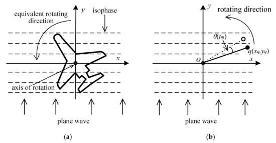
Figure 1.
Rotating platform imaging model of targets. (a) The geometry of an airplane in ISAR imaging, (b) the rotated angle of the scatterer.
The Taylor expressions of and are
where represents the sum of high-order terms of , whose minimum order is . Since is small during the coherent processing time, the quadratic and higher-order terms in (2) and (3) can be ignored. Then, is approximated as
For targets with smooth motion, the uniform rotation model is used to describe after translational motion compensation. The equivalent angular velocity is denoted as , and becomes
In general, an LFM signal is adopted as the transmitted signal, which can be expressed as
where is the pulse width, is the carrier frequency, and is the frequency modulation rate. The bandwidth of the signal is . The rectangular window function satisfies
The echo is received through wideband direct sampling, and then, the matched filtering containing high-speed compensation [29] is adopted for pulse compression. After that, the obtained range profile is expressed as
where is fast time, Q is the total number of scatterers, is the backward scattering coefficient of the ith scatterers, and is light velocity. Function satisfies . Assuming that translational motion compensation has been accomplished, the phase at the peak of the sinc function corresponding to scatterer q is
Clearly, contains two parts: constant phase component and linear phase component. The Fourier transform in the cross-range direction can be used to separate the scatterers in the Doppler frequency domain. The Doppler frequency of scatterer q is , where represents its azimuth position. We denote the range profile sequence after translational motion compensation as , where m represents the pulse number related to and n represents the range cell related to . There are M pulses and N range cells in total. We denote the discrete ISAR image as . The Fourier transform matrix is denoted as P. The process of the range-Doppler algorithm can be expressed as
For targets with complex motion, however, a non-uniform rotation model is used to describe . In general, the angular acceleration, denoted as , and the angular jerk, denoted as , are considered. Herein, the target’s rotation angle is expressed as , and becomes
Therefore, becomes [25,26,27]
Equation (12) indicates that satisfies the PPS model. The target’s complex motion results in quadratic and cubic phase terms in (12), and the corresponding Doppler frequency is time-varying. Consequently, Doppler spreads arise and the ISAR image blurs. In the following section, we analyze and compensate the high-order phase terms of the PPS through non-uniform rotation transform.
3. Properties of the PPS and Rotational Nonuniformity Estimation
In ISAR imaging, the properties of PPS in the cross-range direction need to be addressed. According to (12), the linear, quadratic, and cubic coefficients of a PPS are , , and , respectively. The coefficient ratios and depend on the target’s motion status, and are identical for all scatterers in the target. We name and as RAA and RAJ, respectively. Then, can be expressed as
In (13), angular velocity represents the uniform rotation of the target, and RAA and RAJ represent the non-uniform rotation components. Herein, we select RAA and RAJ as the parameters indicating rotational nonuniformity. To obtain RAA and RAJ, we need to estimate coefficients of PPS.
When the target’s maneuvering is not severe, the PPS model degrades into an LFM signal. In this case, only RAA is considered based on the estimation of linear and quadratic coefficients. The linear and quadratic coefficients of the LFM signal are also referred to as centroid frequency and modulation rate, respectively. According to previous studies, fractional Fourier transform (FrFT) [30], Radon-Wigner transform [31], Lv’s distribution [32], and centroid frequency-chirp rate distribution (CFCRD) [33] are effective approaches for parameter estimation of LFM signals. These methods transform a discrete signal into a two-dimensional parameter domain, and each LFM signal component becomes a two-dimensional peak function. The peak coordinates represent the centroid frequency and modulation rate, respectively. The FrFT algorithm is cross-term free for parameter estimation of multiple LFM signals, but costly for computation, especially for obtaining precise results. CFCRD suffers from cross-term interference under multiple LFM signal components, and yet is efficient in computation cost with fine precision. In this paper, CFCRD is preferred for parameter estimation of multiple LFM signals, and then, a rough value of RAA can be obtained.
When the target’s maneuvering is severe, both RAA and RAJ need to be considered. In this case, coefficients of the CPF signal are estimated. According to previous studies, several algorithms for quadratic and cubic coefficient estimation can be retrieved, such as higher-order ambiguity function-integrated cubic phase function [34], scaled Fourier transform [35], keystone time-chirp rate distribution (KTCRD) [12], and chirp rate-quadratic chirp rate distribution [13]. Similarly, these algorithms transform a discrete signal into a two-dimensional parameter domain whose two dimensions represent quadratic and cubic coefficients, respectively. Considering the trade-off between calculation complexity and estimation precision, the KTCRD method is preferred for quadratic and cubic coefficient estimation of the CPF signal. For a rough estimation, the CFCRD method is still used for linear coefficient estimation of the CPF signal.
Owing to the possible residual error of translational motion compensation, noise interference, cross-term interference, etc., the estimated RAA and RAJ based on individual scatterers are inaccurate. To improve the accuracy, we adopt the averaging scheme. First, several range cells containing strong scatterers are selected for RAA and RAJ estimation. Second, in each range cell, the coefficients of several predominant PPS components are estimated. Then, rough values of RAA and RAJ are obtained. Third, based on the estimated RAAs and RAJs, average RAA and RAJ values are calculated. Through averaging, the estimation errors obtained from individual scatterers are alleviated.
4. New ISAR Imaging Approach based on Optimized Non-Uniform Rotation Transform
In this section, we discuss the implementation of the optimized non-uniform rotation transform and the corresponding ISAR imaging procedures.
With RAA and RAJ, high-order phase terms of the PPS can be constructed and then compensated uniformly in the Fourier transform matrix. Primarily, we concentrate on the compensation of the quadratic phase term in (13), which contains four parameters: . Among them, and are known and indicates the Doppler frequency of scatter q. Through Fourier transform, is projected into cross-range cells in the discrete Doppler domain. Here, we introduce a new variable to represent the discrete value of . Each value corresponds to a row vector in the Fourier transform matrix. For a coherent processing interval containing M pulses, the Fourier transform matrix and values are shown as follows:
 where Note that is proportional to the phase gradient of the row vector in the Fourier transform matrix. With , a row vector in matrix P can be expressed as
where represents the discrete slow time . In fact, is the discrete version of the linear phase term in (13). Similarly, the discrete versions of quadratic and cubic phase terms in (13) can be expressed as
where indicates that is located at the center of the pulse sequence. PRF is short for the pulse repeat frequency. In (16) and (17), PRF is induced by the discretization of . Following are the features of (16) and (17):
where Note that is proportional to the phase gradient of the row vector in the Fourier transform matrix. With , a row vector in matrix P can be expressed as
where represents the discrete slow time . In fact, is the discrete version of the linear phase term in (13). Similarly, the discrete versions of quadratic and cubic phase terms in (13) can be expressed as
where indicates that is located at the center of the pulse sequence. PRF is short for the pulse repeat frequency. In (16) and (17), PRF is induced by the discretization of . Following are the features of (16) and (17):
- (1)
- For all scatterers in the target, the values of , , and are identical.
- (2)
- For scatterers located in the same Doppler cell, their quadratic and cubic phase terms are approximately the same. Consequently, these phase terms can be compensated uniformly using a row vector.
- (3)
- The values of represent the discrete cross-range positions of the scatterers, which are related to different Doppler cells in an ISAR image. When the Doppler frequency of a Doppler cell is zero, is zero. increases with the increment of Doppler frequency.
- (4)
- Different Doppler cells need different compensation components, as expressed in (16) and (17); thus, M sets of and are needed in total. Each set of and is compensated in a row vector of the Fourier transform matrix P.
- (5)
- For the target with smooth motion, both and are zero. No compensation is needed for matrix P.
According to (16) and (17), two compensation matrices can be constructed with the variation of and , which are denoted as and , respectively. The size of and is the same as that of P. The Fourier transform matrix containing high order phase term compensation can be expressed as
where represent Hadamard multiplication and is the non-uniform rotation transform matrix. The imaging formula for targets with complex motion can be expressed as
Given that RAA and RAJ are accurate, an optimal imaging result without blurring can be obtained through (19). However, the estimated RAA and RAJ based on parameter estimation of the PPS are not accurate enough, which degrades the imaging result. To solve this problem, we adopt the parameter searching scheme to obtain optimal RAA and RAJ and an optimal imaging result. First, we set the searching ranges of RAA and RAJ according to the roughly estimated values. Second, we set the searching step lengths according to the accuracy demands. Third, we carry out non-uniform rotation transform based on different RAA and RAJ values, and evaluate the corresponding imaging results using entropy or contrast function (Appendix A). A small entropy and a large contrast indicate good ISAR image quality. According to the imaging result with least entropy or largest contrast, optimal RAA and RAJ and an optimal ISAR image are obtained.
The parameter searching process mentioned above is a brute force solution. Though effective, it is costly in computation. Fortunately, optimal RAA and RAJ corresponding to the optimal imaging result are unique, and thus, the parameter searching process is a convex optimization problem that can be solved through a fast method such as gradient descent. We denote the entropy function of an ISAR image under different RAA and RAJ values as . Partial derivatives and are calculated and then used to update the values of and . When the absolute value of the entropy gradient is smaller than the preset tiny threshold, the entropy is regarded to reach the bottom with optimal RAA and RAJ and an optimal ISAR image.
In the new ISAR imaging approach proposed in this paper, the non-uniform rotation transform instead of conventional Fourier transform is used for cross-range pulse compression. High-order phase terms caused by the target’s complex motion are compensated uniformly in the transform matrix according to (14)–(19). Consequently, the blurring of the ISAR image is eliminated and an optimal imaging result is obtained. Note that the non-uniform rotation transform is a generalized version of conventional Fourier transform. When both RAA and RAJ are zero, the non-uniform rotation transform degrades into conventional Fourier transform. Therefore, our new approach is feasible for ISAR imaging of targets with both smooth and complex motion. The procedure of the new ISAR imaging approach is summarized in Figure 2.
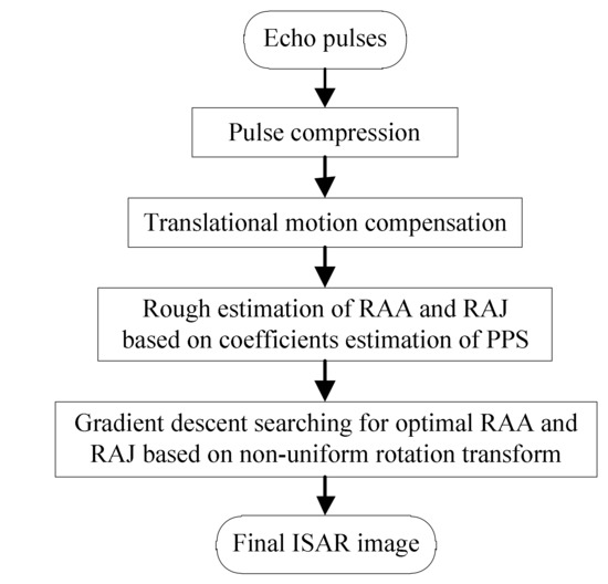
Figure 2.
Procedure of new ISAR imaging approach for targets with complex motion.
5. Experimental Results
In this section, the new imaging approach is validated on the echo pulses of a target with different complex motion. The imaging result of the RID algorithm is considered as comparison.
In the simulation, the parameter settings of the radar system are illustrated in Table 1. The target shown in Figure 3a is a plane model containing 42 scatterers. The backward scattering coefficients of all scatterers are set as 1. Let us assume that the radar is located at the origin of the radar coordinate system O-XYZ, where the O-XY plane is parallel to the horizontal plane. At the starting of the coherent processing interval, the target’s coordinates in the radar coordinate system are (3000, 3000, 7000 m) and its velocity is v = (225, 300, 0)m/s. We set the acceleration of the target to zero. The ISAR image of the target obtained through range-Doppler algorithm is shown in Figure 3b. Obviously, the ISAR image is well focused and it is used as reference for the following experiments.

Table 1.
Parameter settings of the radar system.
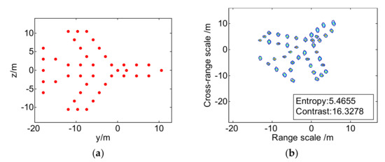
Figure 3.
Target model and ISAR imaging result. (a) Target model; (b) ISAR image of target with smooth motion.
5.1. ISAR Imaging of Target with Constant Acceleration
We set the acceleration of the target as a = (90, 120, 0)m/s2, while the initial velocity and start position of target stay unchanged. The ISAR image obtained through the range-Doppler algorithm is shown in Figure 4a. Compared to Figure 3b, blurring occurs in the ISAR image and the image quality is poor, as indicated by the larger entropy and smaller contrast. The cross-range signal in range cell 485 is extracted and its time-frequency representation is illustrated in Figure 4b. The smoothed pseudo Wigner-Ville distribution [36] is adopted to obtain the time-frequency representation, where it is identified that two scatterers are located in this range cell and the Doppler frequencies of both are time-varying. The slope of the Doppler frequency line is induced by the target’s acceleration. Moreover, the slope of the Doppler frequency line is related to its intercept: larger the intercept, larger is the slope. The relation between the slope and intercept stems from the rigid property of the target body.
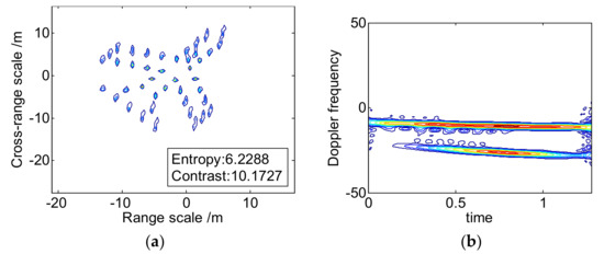
Figure 4.
ISAR imaging result and Doppler frequency of scatterers. (a) ISAR image of target with constant acceleration; (b) time-frequency representation of selected cross-range signal.
The linear Doppler frequency in Figure 4b indicates that the scatterers result in LFM signals, and only RAA needs to be considered. Signals in two range cells are selected, and their parameter distribution through the CFCRD method is shown in Figure 5. The calculation time for the two signals is 3.03 s. Four peaks can be identified in Figure 5a, and three peaks can be identified in Figure 5b. The estimated centroid frequency and modulation rate are illustrated in Table 2. The rough RAA of each scatterer is calculated and the average RAA is found to be 0.1262.
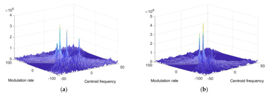
Figure 5.
Parameter estimation of LFM signal. (a) Signal in range cell 506; (b) signal in range cell 465.
Table 2.
Rough RAA values based on parameter estimation of LFM signals.
Next, the gradient descent method is used to obtain the optimal RAA and imaging result. The initial value of RAA is set as 0.1262. Through the iteration process, RAA is updated using , where is the entropy gradient of the ISAR image and the step length is set as 0.001. When the entropy gradient is smaller than , the iteration stops. The RAA and ISAR image in the last iteration are output as the final results. The process and output of the gradient descent process are shown in Figure 6, which shows the entropy to descend gradually. After 51 iterations, the termination condition is met with a calculation time of 4.21 s. The output optimal RAA value is 0.1225. The final ISAR image based on the optimized non-uniform rotation transform is shown in Figure 6b. Compared to that in Figure 4a, the blurring is eliminated effectively and a high-quality ISAR image is obtained, as indicated by the smaller entropy and larger contrast.
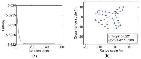
Figure 6.
Search for the optimal RAA and ISAR image through the gradient descent optimization. (a) Entropy change of ISAR image during iteration; (b) optimal ISAR image based on optimized non-uniform rotation transform.
5.2. ISAR Imaging of Target with Curve Flight Path
In this section, the complex motion of the target is set as the curve flight path, as shown in Figure 7a. Non-uniform rotation transform is performed to compensate for the adverse influence of the curve flight path. For simplicity, the attitude of the airplane model is kept constant during imaging. After pulse compression and translation motion compensation, the ISAR image based on the range-Doppler algorithm is obtained as shown in Figure 7b. It can be seen that the curve flight path leads to blurring of the ISAR image. The cross-range signals in range cells 485 and 508 are extracted and their time-frequency representations are illustrated in Figure 8. Two and four scatterers can be identified in these two range cells, respectively. Similar to Figure 4b, the Doppler frequencies in Figure 8 are time-varying. Moreover, the nonlinear feature of the Doppler curve in Figure 8 indicates that the changing rates of the Doppler frequency are not constant. Therefore, the cross-range signals satisfy the CPF model, and both RAA and RAJ need to be estimated.
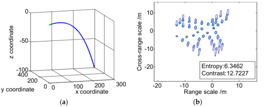
Figure 7.
Targets’ flight path and corresponding ISAR image. (a) Curve flight path of target; (b) ISAR image based on range-Doppler algorithm.
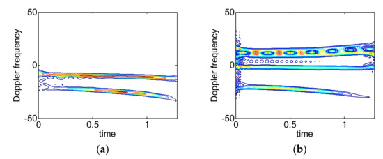
Figure 8.
Time-frequency representation of cross-range signals in the cross-range direction. (a) Signal in range cell 485; (b) signal in range cell 508.
The cross-range signal in range cell 485 is selected to estimate RAA and RAJ. To obtain the coefficients of the CPF signal, CFCRD and KTCRD are carried out as shown in Figure 9. According to Figure 9a, the centroid frequency and modulation rate of the two scatterers are (10, 2.745) and (24.12, 6.667), respectively. Thus, the rough RAA value is 0.27. According to Figure 9b, the modulation rate and quadratic modulation rate of the two scatterers are (2.5, 2) and (8, 10), respectively. Then, we obtain . In other words, RAJ/RAA ≈ 1, so a rough RAJ value is also 0.27.
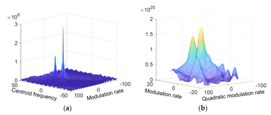
Figure 9.
Parameter estimation of the PPS. (a) Estimation of linear and quadratic coefficients; (b) estimation of quadratic and cubic coefficients.
To demonstrate the effect of RAA and RAJ compensation, two schemes are carried out. In the first scheme, only RAA compensation is considered in the gradient descent process, and the results are illustrated in Figure 10. The minimum ISAR image entropy is 5.8337 after 71 iterations. The calculation time is 5.84 s and the output RAA is 0.1443. Compared to Figure 7b, the ISAR image in Figure 10b shows a significant improvement. However, slight blurring can still be identified, as indicated by a red dash circle in Figure 10b. In the second scheme, both RAA and RAJ are considered and a two-dimensional gradient descent process is carried out. In each iteration, RAA is updated using and RAJ is updated using , where the step length is set as 0.002. Between two adjacent iterations, if the entropy change is smaller than 0.0001, the iteration process stops. The initial values of both RAA and RAJ are set as 0.27. The termination condition is met after 61 iterations, as shown in Figure 11a, and the calculation time is 16.43 s. The outputs of optimal RAA and RAJ are 0.1766 and 0.2075, respectively. The entropy of the output ISAR image shown in Figure 11b is smaller than that in Figure 10b. A larger contrast of Figure 11b also indicates that a better image quality is obtained.
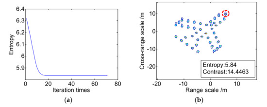
Figure 10.
Search for optimal RAA and imaging result through gradient descent method. (a) Entropy of ISAR image during iteration; (b) output ISAR image.
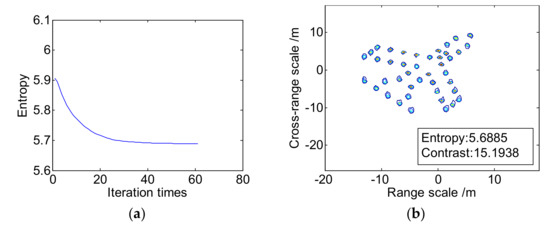
Figure 11.
Search for optimal imaging result through two-dimensional gradient descent process. (a) Entropy of ISAR image during iteration; (b) output ISAR image.
We can conclude that for the target’s complex motion on such a curve flight path, the cross-range signal satisfies the CPF signal model. Using a non-uniform rotation transform containing only RAA compensation, the blurring of the ISAR image is alleviated, but slight blurring still exists. When both RAA and RAJ are considered in the non-uniform rotation transform, an optimal ISAR image is obtained. Herein, we conclude that the proposed optimized non-uniform rotation transform is effective for ISAR imaging of targets with complex motion.
5.3. ISAR Imaging of Boeing 727 with Complex Motion
We also test the non-uniform rotation transform on the simulated data of Boeing B727 airplane provided by the U.S. Naval Research Laboratory [5]. The data contain 256 successive pulses, as shown in Figure 12a. The carrier frequency is 9 GHz, the bandwidth is 150 MHz, and PRF is 20 KHz. The total coherent processing time is 0.0128 s. Translational motion compensation has been accomplished. Because of the maneuvering of the target, the ISAR image obtained through the range-Doppler algorithm is blurred as shown in Figure 12b. To overcome the blurring, the optimized non-uniform rotation transform is carried out and its imaging result is compared with that of the RID algorithm.
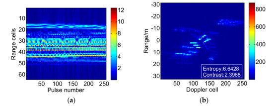
Figure 12.
Data of Boeing 727. (a) 256 echo pulses; (b) ISAR image based on range-Doppler algorithm.
Primarily, rotational nonuniformity needs to be estimated. The time-frequency distribution of the cross-range signal in range cell 31 is obtained through the smoothed pseudo Wigner-Ville distribution, as shown in Figure 13a. The linear curves in the figure indicate that the signal satisfies the LFM model, thus only RAA needs to be estimated. Due to the short duration of the cross-range signal, CFCRD is not suitable for coefficient estimation in this case. Alternatively, FrFT [37] is used to estimate the signal coefficient as shown in Figure 13b. The centroid frequency and modulation rate of the two scatterers shown in Figure 13b are (−745, −24,546) and (1375.7, 98,304), respectively. Then, the rough RAA value is 26.2. Next, the gradient descent process is carried out to obtain the optimal RAA and imaging result. The step length in iteration is set as 1 and the termination condition is set such that the entropy gradient is smaller than 1 × 10⁻⁶. After 352 iterations, the termination condition is met and the calculation time is found to be 7.22 s; the output optimal RAA value is 32.24. The entropy change during the iteration and the output optimal ISAR image are shown in Figure 14. Compared to Figure 12b, the blurring in Figure 14b is eliminated significantly. The change in entropy and contrast also verifies the effectiveness of the proposed algorithm.
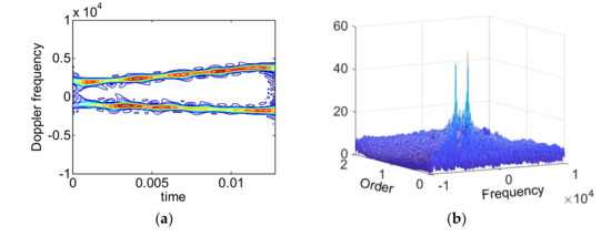
Figure 13.
Frequency components of cross-range signal in a range cell. (a) Time-frequency representation; (b) FrFT distribution.
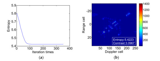
Figure 14.
Search for optimal RAA and imaging result through gradient descent method. (a) Entropy of ISAR image during iteration; (b) output ISAR image.
In contrast, an RID algorithm is used to obtain the instantaneous ISAR image of Boeing 727. In each range cell, the cross-range signal is processed with smoothed pseudo Wigner-Ville distribution to obtain the two-dimensional time-frequency distribution. At each time instant, the instantaneous Doppler frequencies of the cross-range signals in 64 range cells combine an RID ISAR image. There are 256 RID ISAR images in total, of which two representative images, 8th and 30th, are illustrated in Figure 15. Compared to the image shown in Figure 12b, blurring is eliminated significantly in the images shown in Figure 15. However, the defects are also obvious. First, Doppler spread of individual scatterers still exists, which can be identified in Figure 15a. Second, weak scatterers become almost invisible, which leads to the loss of target shape information. It is difficult to interpret an airplane from Figure 15b. Third, the RID image is unstable since images at different time instants are different. It is found that entropy and contrast are not proper norms for selecting the best one from 256 RID images. This leads to confusion and inconvenience in practice.
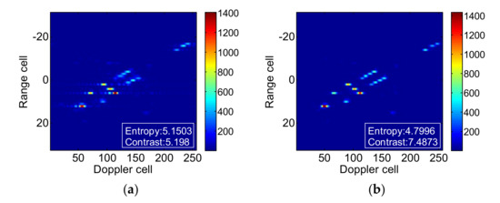
Figure 15.
RID image based on smoothed pseudo Wigner-Ville distribution. (a) At time instant 0.0005 s; (b) at time instant 0.0015 s.
The ISAR image observed in Figure 14b is still better than the RID images observed in Figure 15. Though entropy and contrast of the latter indicate better image quality, the former provides clearer and more stable target information. This confirms the advantages of non-uniform rotation transform over the RID algorithm. Table 3 compares three algorithms. In summary, the proposed method outperforms range-Doppler and RID algorithms in terms of the image quality. Moreover, the imaging result of the proposed method is unique and more stable compared to that of RID.
Table 3.
Algorithm comparison.
6. Conclusions
In this paper, a new imaging approach based on an optimized non-uniform rotation transform is proposed for ISAR imaging of targets with complex motion. Two parameters, RAA and RAJ, are defined to describe the equivalent rotational nonuniformity of the target. Based on RAA and RAJ, the quadratic and cubic phase terms resulting from the target’s complex motion can be compensated uniformly in the Fourier transform matrix. A rough estimation of RAA and RAJ is realized through coefficient estimation of the PPS. The optimal RAA and RAJ are obtained through gradient descent optimization, after which an optimal ISAR image is obtained. In this way, ISAR imaging of the target with complex motion is converted into the parameter optimization problem. Through the optimized nonuniformity rotation transform, the blurring in the ISAR image of the target with complex motion is eliminated effectively. Compared to precedent imaging algorithms such as RID algorithm, the imaging result of the proposed method is clearer and more stable. Moreover, the additional computation cost of the proposed method is reasonable. Imaging results of targets with different complex motion and simulated data of Boeing 727 verify the effectiveness and advantages of the proposed algorithm. Our future work focuses on the possible adverse influence and countermeasures of translational motion compensation error on non-uniform rotation transform.
Supplementary Materials
The simulated echo pulses of Boeing 727 shown in Figure 12 are available online at http://www.mdpi.com/2072-4292/10/4/593/s1.
Acknowledgments
This work was supported by the National Natural Science Foundation of China (No. 61471373).
Author Contributions
Wenzhen Wu and Shiyou Xu propose the method, conceived and designed the experiments; Wenzhen Wu performed the experiments and wrote the paper; Wenzhen Wu, Pengjiang Hu and Jiangwei Zou analyzed the data; Pengjiang Hu, Jiangwei Zou and Zengping Chen revised the paper.
Conflicts of Interest
The authors declare no conflict of interest. The founding sponsors had no role in the design of the study; in the collection, analyses, or interpretation of data; in the writing of the manuscript, and in the decision to publish the results.
Appendix A
The mathematic definition of ISAR image entropy used in this paper is:
where represents ISAR image, N and M represent the total number of range cells and cross-range cells of the ISAR image, respectively. In a similar manner, the mathematical definition of the ISAR image contrast is:
where represents the average operation.
References
- Chen, V.C.; Andrews, H.C. Target-motion-induced radar imaging. IEEE Trans. Aerosp. Electron. Syst. 1980, 16, 2–14. [Google Scholar] [CrossRef]
- Chen, V.C.; Martorella, M. Introduction to ISAR imaging. In Inverse Synthetic Aperture Radar Imaging Principles, Algorithms and Applications; SciTech Publishing: Edison, NJ, USA, 2014; pp. 1–19. [Google Scholar]
- Tian, B.; Zou, J.; Xu, S.; Chen, Z. Squint model interferometric ISAR imaging based on respective reference range selection and squint iteration improvement. IET Radar Sonar Navig. 2015, 9, 1366–1375. [Google Scholar] [CrossRef]
- Tian, B.; Liu, Y.; Xu, S.; Chen, Z. Analysis of synchronization errors for InISAR on sepatated platforms. IEEE Trans. Aerosp. Electron. Syst. 2016, 52, 237–244. [Google Scholar] [CrossRef]
- Wang, Y.; Ling, H.; Chen, V.C. ISAR motion compensation via adaptive joint time–frequency technique. IEEE Trans. Aerosp. Electron. Syst. 1997, 34, 670–677. [Google Scholar] [CrossRef]
- Thayaparan, T.; Brinkman, W.; Lampropoulos, G. Inverse synthetic aperture radar image focusing using fast adaptive joint time–frequency and three-dimensional motion detection on experimsental radar data. IET Signal Process. 2009, 4, 382–394. [Google Scholar] [CrossRef]
- Chen, V.C.; Qian, S. Joint time–frequency transform for radar range-Doppler imaging. IEEE Trans. Aerosp. Electron. Syst. 1998, 3, 486–499. [Google Scholar] [CrossRef]
- Wang, Y.; Jiang, Y.C. ISAR imaging of maneuvering target based on the L-Class of fourth-order complex-lag PWVD. IEEE Trans. Geosci. Remote Sens. 2010, 48, 1518–1527. [Google Scholar] [CrossRef]
- Li, D.; Liu, H.; Gui, X.; Zhang, X. An efficient ISAR imaging method for maneuvering target based on synchrosqueezing transform. IEEE Antennas Wirel. Propag. Lett. 2016, 15, 1317–1320. [Google Scholar] [CrossRef]
- Liu, Z-S.; Wu, R.; Li, J. Complex ISAR imaging of maneuvering targets via the Capon estimator. IEEE Trans. Signal Process. 1999, 47, 1262–1271. [Google Scholar]
- Zheng, J.B.; Su, T.; Zhu, W.; Liu, Q.H. ISAR imaging of targets with complex motions based on the keystone time-chirp rate distribution. IEEE Geosci. Remote Sens. Lett. 2014, 11, 1275–1279. [Google Scholar] [CrossRef]
- Zheng, J.B.; Su, T.; Zhang, L.; Zhu, W.; Liu, Q.H. ISAR imaging of targets with complex motion based on the chirp rate–quadratic chirp rate distribution. IEEE Geosci. Remote Sens. 2014, 52, 7276–7289. [Google Scholar] [CrossRef]
- Bao, Z.; Wang, G. Inverse synthetic aperture radar imaging of maneuvering targets based on Chirplet decomposition. Opt. Eng. 1999, 37, 1582–1588. [Google Scholar] [CrossRef]
- Wang, Y.; Jiang, Y.-C. ISAR imaging for three-dimensional rotation targets based on adaptive Chirplet decomposition. Multidimens. Syst. Signal Process. 2010, 21, 59–71. [Google Scholar] [CrossRef]
- Wang, Y.; Jiang, Y.-C. Modified adaptive Chirplet decomposition with application in ISAR imaging of maneuvering targets. EURASIP J. Adv. Signal Process. 2008, 1–8. [Google Scholar] [CrossRef]
- Sun, C.; Bao, Z. Super-resolution algorithm for instantaneous ISAR imaging. Electron. Lett. 2000, 36, 253–255. [Google Scholar]
- Stoica, P.; Li, J.; Ling, J. Missing data recovery via a nonparametric iterative adaptive approach. IEEE Signal Process. Lett. 2009, 16, 241–244. [Google Scholar] [CrossRef]
- Wang, X.; Zhang, M.; Zhao, J. Super-resolution ISAR imaging via 2D unitary ESPRIT. Electron. Lett. 2015, 51, 519–521. [Google Scholar] [CrossRef]
- Hu, P.; Xu, S.; Wu, W.; Tian, B.; Chen, Z. IAA-based high-resolution ISAR imaging with small rotational angle. IEEE Geosci. Remote Sens. Lett. 2017, 14, 1978–1982. [Google Scholar] [CrossRef]
- Zhang, L.; Xing, M.; Qiu, C.-W.; Li, J.; Bao, Z. Achieving higher resolution ISAR imaging with limited pulses via compressed sampling. IEEE Geosci. Remote Sens. Lett. 2009, 6, 567–571. [Google Scholar] [CrossRef]
- Zhang, L.; Xing, M.; Qiu, Ch.; Li, J.; Sheng, J.; Li, Y.; Bao, Z. Resolution enhancement for inversed synthetic aperture radar imaging under low SNR via improved compressive sensing. IEEE Trans. Geosci. Remote Sens. 2010, 48, 3824–3838. [Google Scholar] [CrossRef]
- Cohen, L. Time-frequency distributions—A review. Proc. IEEE 1989, 77, 941–981. [Google Scholar] [CrossRef]
- Munoz-Ferreras, J.M.; Perez-Martınez, F. Non-uniform rotation rate estimation for ISAR in case of slant range migration induced by angular motion. IET Radar Sonar Navig. 2007, 1, 251–260. [Google Scholar] [CrossRef]
- Wang, Y.; Lin, Y. ISAR imaging of non-uniformly rotating target via Range-Instantaneous-Doppler-Derivatives algorithm. IEEE J. Sel. Top. Appl. Earth Obs. Remote Sens. 2014, 7, 167–176. [Google Scholar] [CrossRef]
- Wang, Y.; Zhao, B. Inverse synthetic aperture radar imaging of non-uniformly rotating target based on the parameters estimation of multi-component quadratic frequency-modulated signals. IEEE Sens. J. 2015, 15, 4035–4061. [Google Scholar] [CrossRef]
- Li, D.; Zhan, M.; Zhang, X.; Fang, Z.; Liu, H. ISAR imaging of nonuniformly rotating target based on the multicomponent CPS model under low SNR environment. IEEE Trans. Aerosp. Electron. Syst. 2017, 53, 1119–1135. [Google Scholar] [CrossRef]
- Liu, L.; Qi, Mi.; Zhou, F. A novel non-uniform rotational motion estimation and compensation method for maneuvering targets ISAR imaging utilizing particle swarm optimization. IEEE Sens. J. 2018, 18, 299–309. [Google Scholar] [CrossRef]
- Jorge, N.; Wright, S.J. Numerical Optimization; Springer Science & Business Media: Medford, MA, USA, 2006; pp. 30–42. [Google Scholar]
- Tian, B.; Liu, Y.; Xu, S.; Chen, Z. Interferometric inverse synthetic aperture radar imaging for space targets based on wideband direct sampling using two antennas. J. Appl. Remote Sens. 2014, 8, 083599. [Google Scholar] [CrossRef]
- Almeida, L.B. The fractional fourier transform and time-frequency representations. IEEE Trans. Signal Process. 1994, 42, 3084–3091. [Google Scholar] [CrossRef]
- Wood, C.; Barry, T. Radon transformation of time-frequency distributions for analysis of multicomponent signals. IEEE Trans. Signal Process. 1994, 42, 3166–3177. [Google Scholar] [CrossRef]
- Lv, X.L.; Bi, G.A.; Wang, C.; Xing, M. Lv’s distribution: Principle, implementation, properties, and performance. IEEE Trans. Signal Process. 2011, 59, 3576–3591. [Google Scholar] [CrossRef]
- Zheng, J. Research on the ISAR imaging based on the non-searching estimation technique of motion parameters. Chapter 2. Ph.D. Dissertation, Xidian University, Xi’an, China, 2014. [Google Scholar]
- Wang, Y. Inverse synthetic aperture radar imaging of maneuvering target based on range-instantaneous-doppler and range-instantaneous-chirp-rate algorithms. IET Radar Sonar Navig. 2012, 6, 921–928. [Google Scholar] [CrossRef]
- Bai, X.; Tao, R.; Wang, Z.J.; Wang, Y. ISAR imaging of a ship target based on parameter estimation of multicomponent quadratic frequency-modulated signals. IEEE Trans. Geosci. Remote Sens. 2014, 52, 1418–1429. [Google Scholar] [CrossRef]
- Wu, Y.; Munson, D.C. Wide-angle ISAR passive imaging using smoothed pseudo Wigner-Ville distribution. In Proceedings of the IEEE Radar Conference, Atlanta, GA, USA, 3 May 2001; pp. 363–366. [Google Scholar]
- Ozaktas, H.M.; Arikan, O.; Kutay, M.A.; Bozdagt, G. Digital computation of the fractional fourier transform. IEEE Trans. Signal Process. 1996, 44, 2141–2150. [Google Scholar] [CrossRef]


© 2018 by the authors. Licensee MDPI, Basel, Switzerland. This article is an open access article distributed under the terms and conditions of the Creative Commons Attribution (CC BY) license (http://creativecommons.org/licenses/by/4.0/).