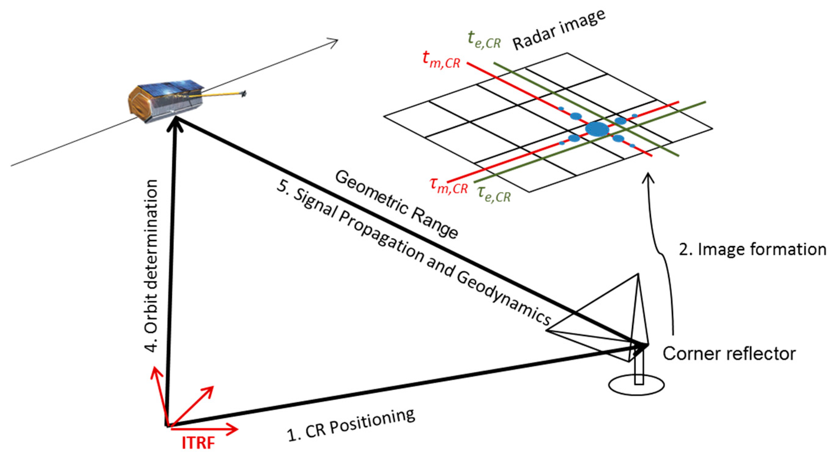
4.1. Monitoring the Operational Readiness of a CR
A lesson learned from our long-term measurement series, is to be aware of weather influences affecting the performance of a CR [
21]. Snow within the CR changes the backscatter geometry and in consequence firstly lowers the CR’s RCS and secondly—much more problematic for our measurements—it changes the actual position of the CR phase center. Because the CR models we installed have drainage holes at their converging corners, rain is in general not a problem, except when leaves fallen or blown into the CR may clog the drainage hole.
As the significantly lowered RCS is a good indicator for such disturbances, we routinely monitor the RCS and compare its value against the expected value derived from theory or experience. Based on an empirically derived threshold of 3 dB RCS loss relative to the expected value, we are able to identify the TerraSAR-X measurements affected by such irregular conditions and exclude them from further analyses, where they would otherwise occur as coarse (i.e., decimeter-level) outliers. During our analysis we did not observe any significant correlation of moderate RCS losses of less than 3 dB with the shifts in the SAR measured CR locations.
Over the course of our investigations and based on this assumption, we identified in total 79 disturbed location measurements, reducing the number of datatakes in the analysis from 1060 to 981. In contrast, there still remain 18 measurements (approximately 1.8%) with a conspicuously high location error of 7‒11 cm where no obvious external cause could be identified. With the exception of one, these values are found in azimuth. Because we have no indication for an external cause, these measurements must not be excluded from analysis.
4.2. Geometric Recalibration Constants
We have chosen the CR at the Metsähovi test site as the reference for our TerraSAR-X recalibration. Here, the mounting of the CR on stable bedrock provides confidence that the geodetic coordinates of its phase center are even more long-term stable than the ones from our other test sites. Because the measurement series are in HH polarization mode, we originally focused our recalibration activities on this mode and just recently complemented them by deriving recalibration constants for VV polarization too.
Table 3 shows our new calibration constants to be applied by the user. To remain consistent with the sign convention of the operational calibration constants, our recalibration constants have to be subtracted from the measured radar times at all test sites (i.e., the absolute value of the negative constants has to be added!). For convenience,
Table 3 also shows the values converted to distances. Note that we use an average ground track velocity as conversion factor for azimuth here, whereas the precise value in a given SAR image depends on geometric factors like the incidence angle and the topographic height.
In addition to the operational range calibration constant that is already implicitly applied during TerraSAR-X image focusing, we had to introduce a range recalibration constant that the user has to apply explicitly. The amount of our range recalibration constant corresponds to about 30 cm spatial distance, see
Table 3. The cause for its necessity can be found mainly in the different handling of the wet part of the tropospheric delay in both measurement concepts. Being the most volatile contribution to the tropospheric delay, its consideration is beyond the capabilities of the simplified model underlying the annotated delay value and in consequence, it contributes in average to the operational calibration constant. When we make use of the measured tropospheric delay of the IGS, the wet delay is already included and must not be considered twice. Thus, our recalibration constant figures as a readjustment of the wet delay’s contribution in the operationally applied calibration constant.
The likely explanation for the small difference of 0.27 nanoseconds (equivalent to 4 cm) discovered in the range calibration constants of both polarization channels (cf.
Table 3) might be found in the staggered mounting of H and V antenna elements on the satellite’s surface and in the slightly different signal routing inside the sensor electronics.
In contrast to the range, the operational calibration constant in azimuth is not applied in the processor; hence a user is able to replace it with our new constants. The differences between the results of the operational calibration and our recalibration are rather small (corresponding to about 11 mm spatial distance for TSX-1 and 6 mm for TDX-1). However, we benefit from the long duration of our measurement series, the more precisely determinable CR reference coordinates in the vicinity to the IGS reference stations, and from the firm orientation of the CRs that avoids any undesirable change of their phase centers. Due to these factors, we were able to slightly refine the azimuth calibration constants of both sensors.
Finally, we want to give some remarks on the cross-polar channels. Because trihedral CRs do not change the plane of polarization, our CRs are invisible in cross-polar image channels, as they are employed in polarimetry. Consequently, a geometric recalibration of the cross-polar channels HV and VH is out of the capabilities of our on-ground measurement equipment, but we can provide assumptions about adequate recalibration constants for the cross-pol channels based on theoretical considerations. Assuming that most of the differences between the examined co-polar channels HH and VV results from construction particulars of the antenna and the sensor electronics, we might conclude that the recalibration constants for HV and VH are approximately in the mean of the HH and VV constants, because HV shares the transmit path with the HH channel and the receive path with the VV channel, while the opposite is true for VH.
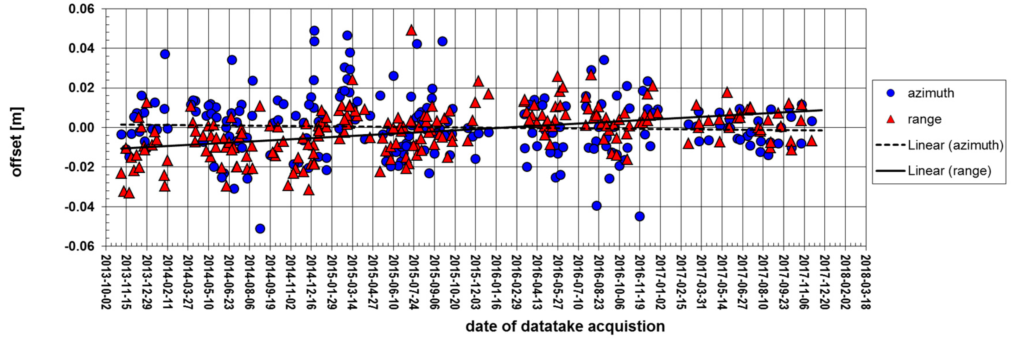
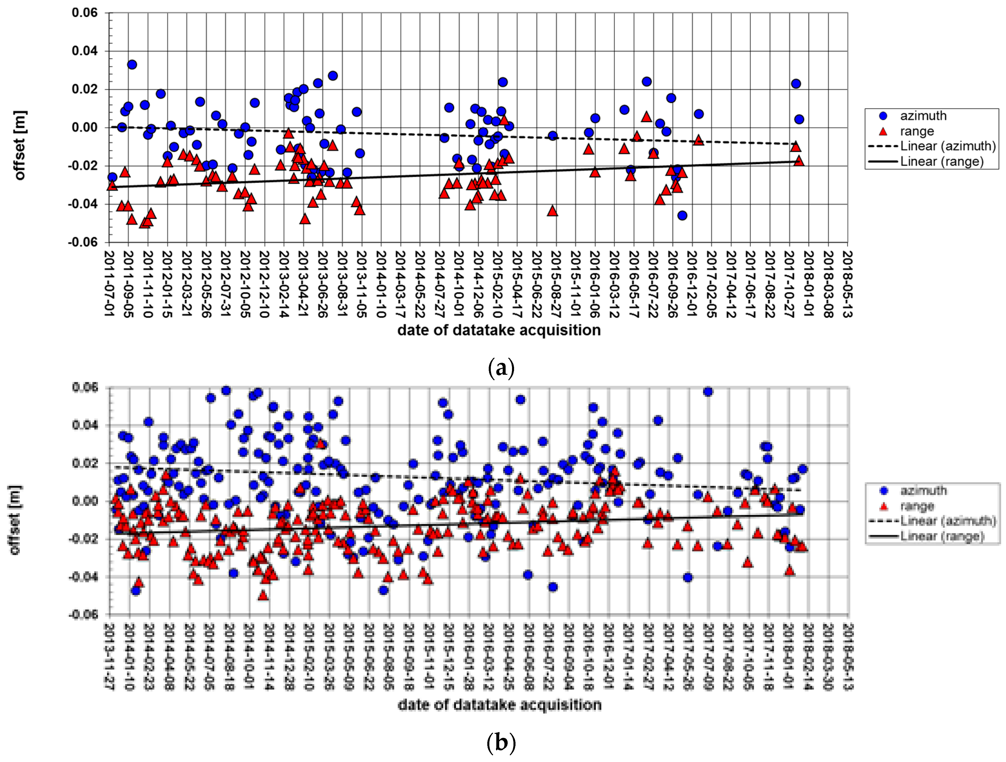
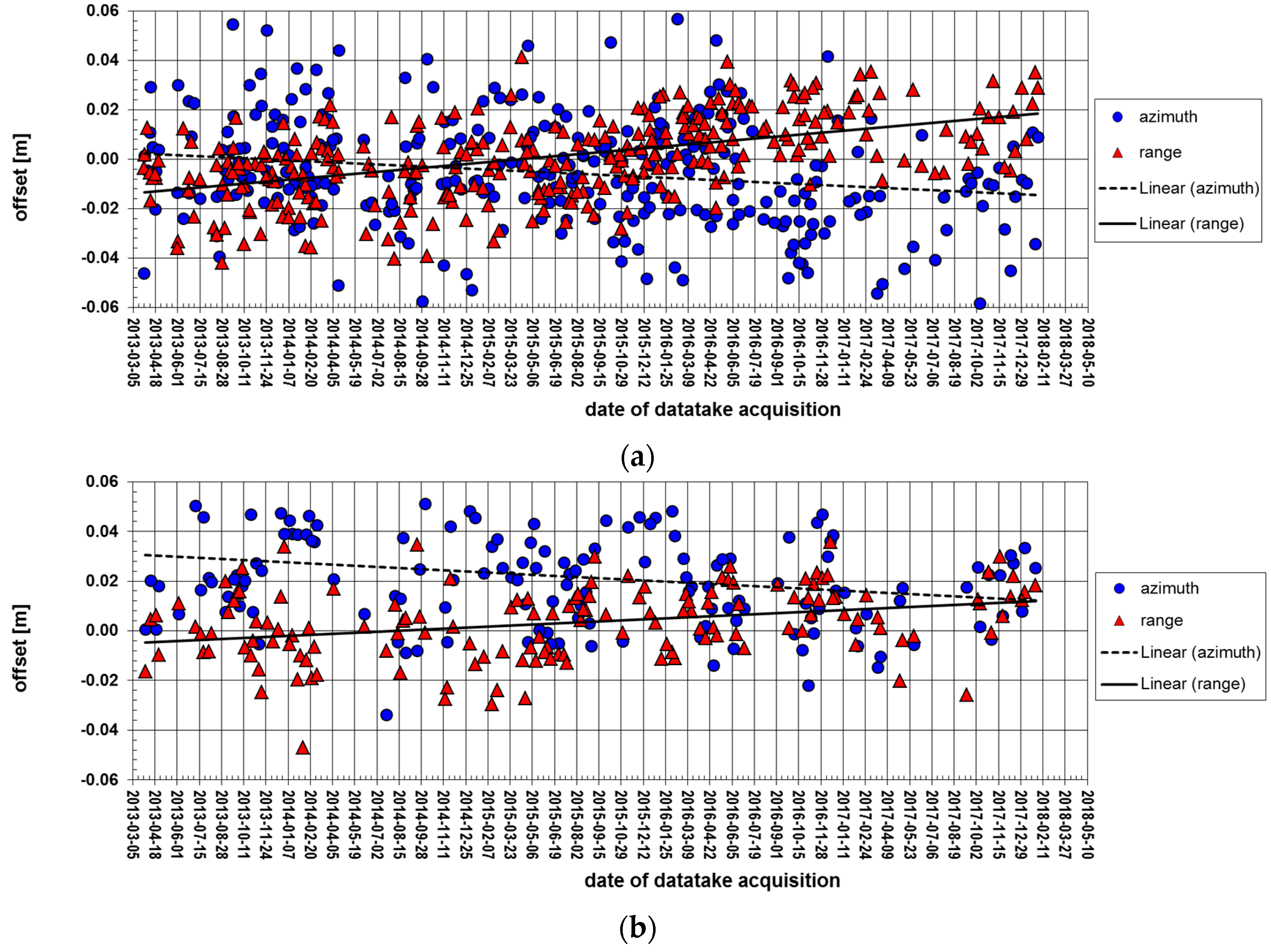
4.3. Temporal Stability of SAR Geolocation Results
Figure 3,
Figure 4 and
Figure 5 show the temporal progression of the azimuth and range offsets between measured and expected radar coordinates at our three test sites. A slight trend is perceivable from all plots. In all measurement series, there is a tendency of the measured values toward early azimuth and toward far range. In order to estimate the magnitude of this trend, we approximated the temporal progressions of the offsets by a linear function and investigated the obtained gradients.
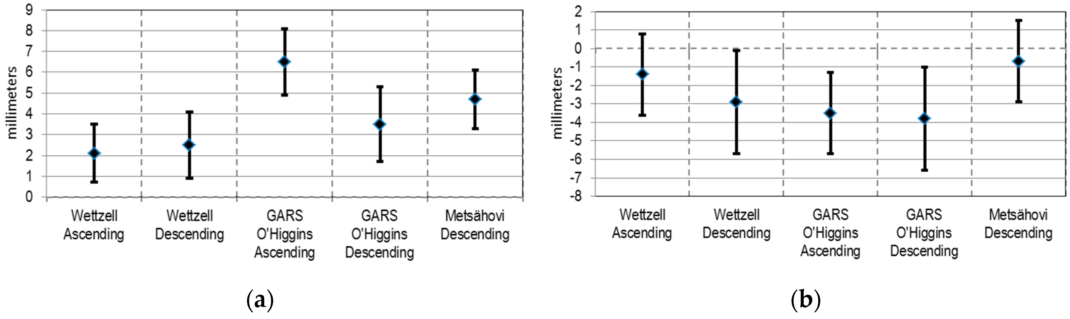
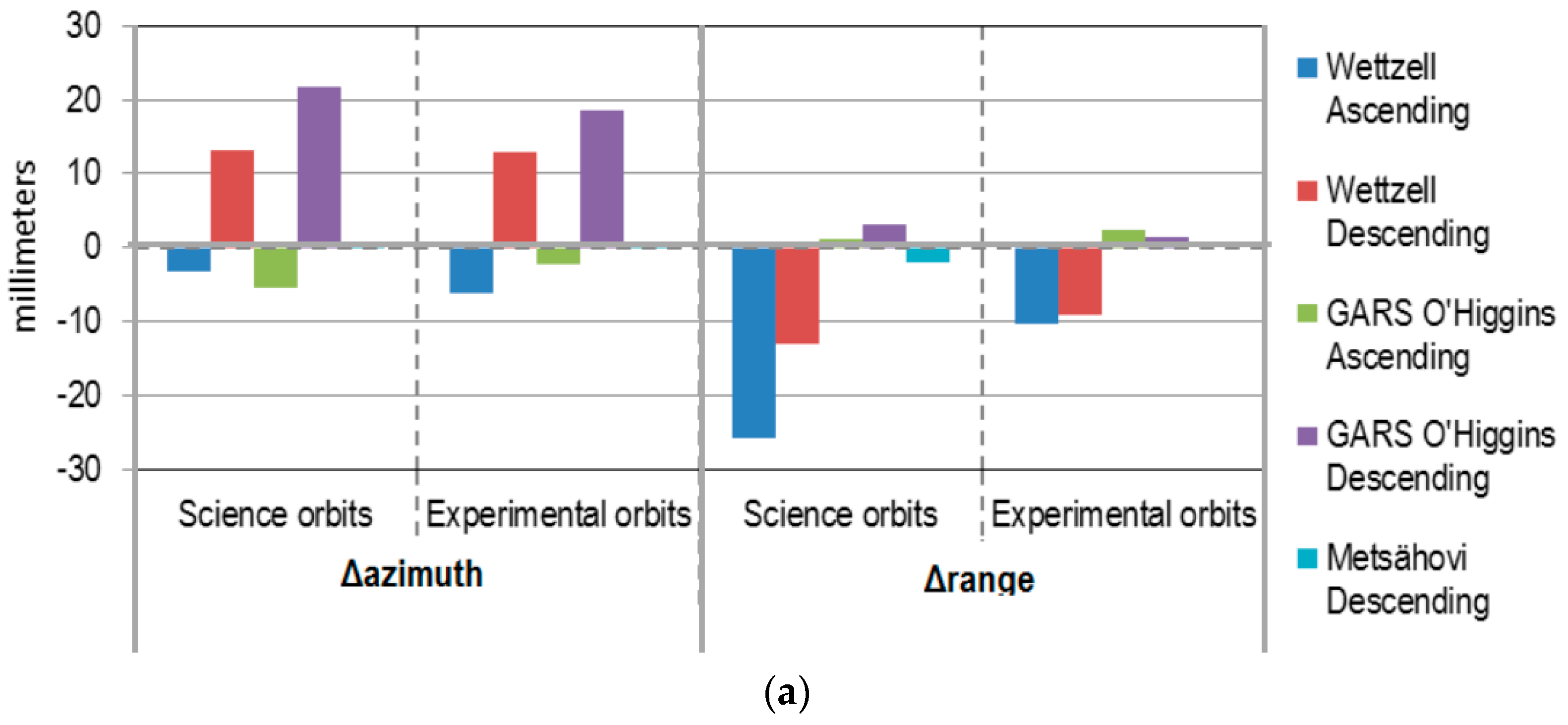
Table 4 and
Figure 6 show that the gradients are in the order of millimeters per year and exceed the standard deviation (1σ) expected from error propagation. However, the 1σ just represents a 68% confidence interval whereas for a 95% confidence interval 2σ is required [
15]. The gradients in range even exceed 3σ so that a confidence level of more than 99.7% results. Therefore we consider the range effect to be significant. For the azimuth, the results from the different test sites are much less distinct and some of the estimated gradients (Wettzell Ascending and Metsähovi Descending) obviously remain below the 2σ, thus the continuation of the ongoing measurement series is required to reduce the remaining uncertainty.
Assuming that the trend in the range measurements is real, finding a possible cause for it is subject of ongoing investigations. We may already excluded some potential causes: The stability of the sensor internal clock rate governing all timings in the SAR payload is routinely monitored in the TerraSAR-X mission and in this way known with nine digit accuracy (the technique is described in [
27]). In consequence, this error contribution cannot exceed 3 mm and is therefore below the amount of the observed trends. Also the satellite orbit determination is not considered to be a cause because we have independent measurements of the TerraSAR-X orbits based on Satellite Laser Ranging (SLR) confirming the long-term stability—see [
28] for more. Thus, the focus of our further investigations has to be on the SAR sensor itself. We might investigate e.g., whether slight aging effects in electronic components are supposable. The challenge is that to our knowledge no prior space-borne SAR sensor was examined after insert to orbit at a comparable level of detail.
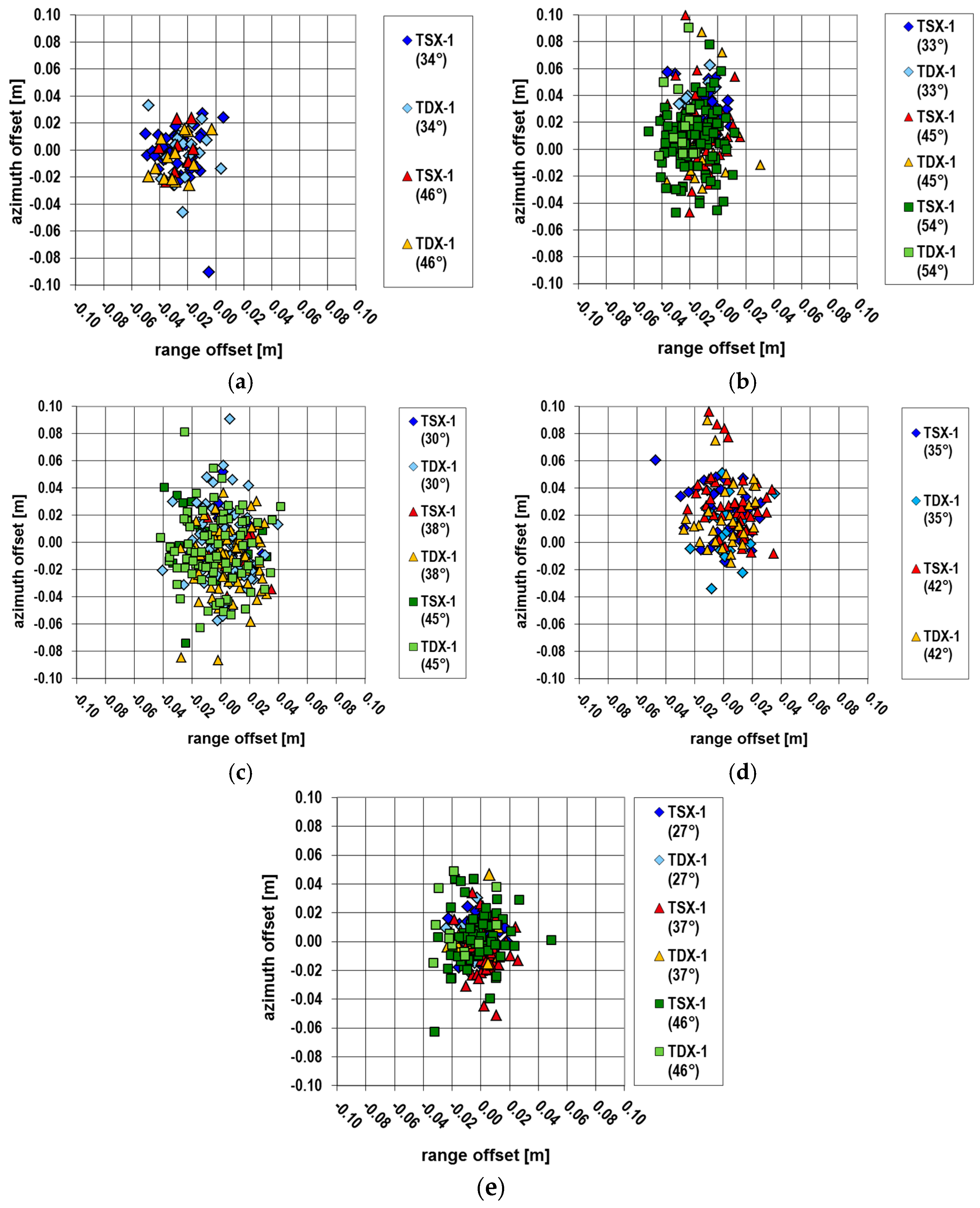
4.6. Location Independency of Results
Table 6 shows the overall mean values and standard deviations of the localization error determined at our different test sites. As Metsähovi is used as our recalibration reference, the mean location offset is consequently close to zero and does not contain any useful information. However, the standard deviation determined at this test site is not influenced by the recalibration and therefore it is still an independent measurement result.
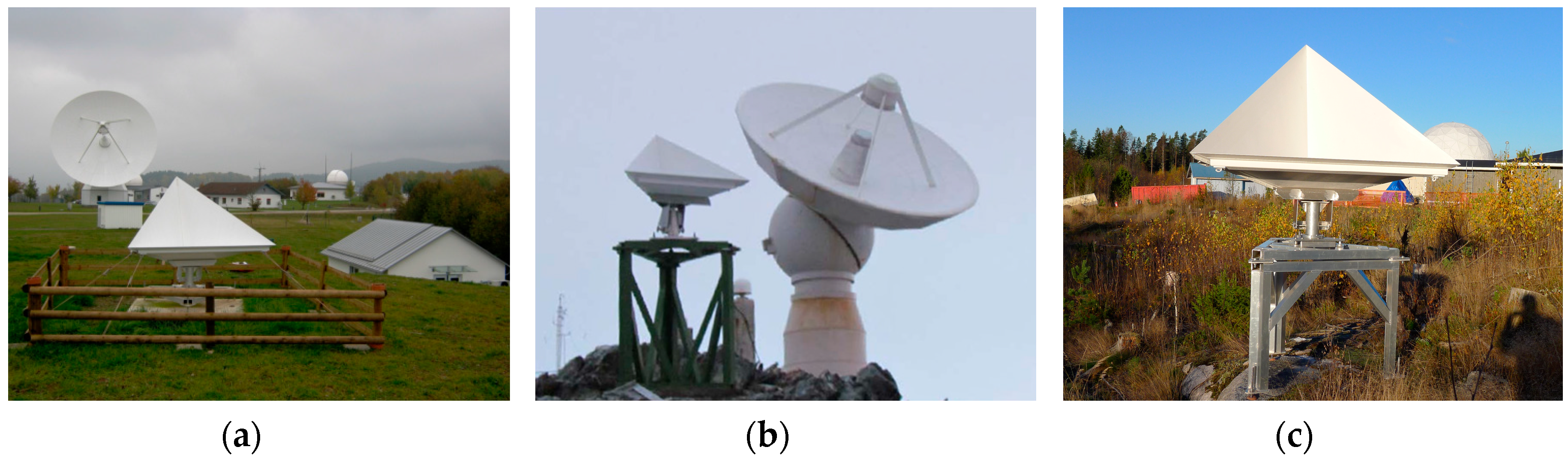
The obtained mean values at the other test sites indicate the consistency between SAR location measurements and the calibration derived for Metsähovi. They amount from few millimeters up to 2.6 cm. The maximum range bias results for the Wettzell Ascending CR. However, a terrestrial resurvey of this reflector disclosed the cause for the deviating behavior of this single measurement series: The concrete foundation of the CR subsided by about 2 cm during the first 2 years after the CR was installed and surveyed. While we chose the location for our first CR with regard to a minimum disturbance in the radar image from the installations of the IGS reference station, we did not take enough care of the ground conditions and put the foundation on a small mound rising above the local surroundings, see
Figure 2a. As lesson learned, we more carefully considered this aspect when installing the other CRs.
The standard deviations of the single measurement series in range vary from 12 to 18 mm. The standard deviation in azimuth is somewhat higher and ranges from 18 to 25 mm, which is still nearly two orders of magnitude below the upper limit defined in the TerraSAR-X product specification [
24]. The lower performance of the azimuth localization accuracy is limited by the annotation precision (18.6 microseconds step width) of the raw data acquisition time. Even if it is derived from very accurate pulse per seconds (PPS) information of the on-board GPS receivers [
27], the information is stored in the SAR payload with an insufficient number of digits. We strongly recommend future SAR missions to provide a finer time annotation. For TerraSAR-X we found a way to overcome the truncated timing by applying a post processing of the azimuth timing [
27]. Since May 2014, this post processing is part of the operational TerraSAR-X SAR processor and lowers the quantization error of the azimuth timing by about one order of magnitude. The remaining error amounts to about 1 microsecond, equivalent to about 7 mm azimuth location error.
Comparing the standard deviations obtained at the different test sites, the 0.7 m CRs at GARS O’Higgins are inferior to the 1.5 m CRs at Wettzell and Metsähovi as it is predicted from theoretical considerations because of the lower RCS resulting in a lower SCR. Using Equation (3) and inserting the parameters of our (HS300) measurement series at GARS O’Higgins or Wettzell and Metsähovi, respectively, the expected clutter contribution to the overall location error in case of a 0.7 m reflector amounts to 6 mm in range and 12 mm in azimuth. In case of a 1.5 m CR the values read 1.0 and 1.8 mm, respectively. Thus, a good deal of the difference in the standard deviations is explainable by the different CR sizes.
4.7. 3-D Coordinates
The solution of the independent SAR positioning with TerraSAR-X at the test sites can be directly compared to the coordinates from the surveys. To ease interpretation, the differences in global X, Y and Z have been rotated to the local north, east, and height frame of the respective station. Since we removed the average ITRF station velocity in the processing (see
Section 2.1), the SAR coordinates are reduced to the epoch of the first SAR datatake in the series. Therefore, we transformed the reference ITRF2014 coordinates of the CRs to this epoch to ensure a consistent comparison.
The coordinate differences listed in
Table 7 confirm the very high accuracy of the TerraSAR-X positioning ability, if all the known contributions have been compensated for in the measurements and if the sensors are accurately calibrated. Naturally, the differences for the Metsähovi CR are very small because this reflector was used to derive the calibration constants (see
Section 4.2). At the other test sites, the remaining differences are usually in the order of 1‒2 cm, while the largest difference of 4 cm is found for the east component of the GARS O’Higgins Descending CR. However, when examining the estimated standard deviations, the reason for this becomes clear. Like the Wettzell Ascending reflector, this reflector is only captured by two passes (see
Table 5), and the smaller baseline between the two adjacent passes results in a larger uncertainty for the east component. In addition, one would also expect an impact of the reflector size (0.7 m versus 1.5 m), but this is mostly compensated by the larger number of acquisitions at GARS O’Higgins.
The comparison of the coordinate differences with the 95% confidence interval also listed in
Table 7 shows that only a few of the differences are actually significant. The overall error behavior of a higher quality in the north component and a reduced quality for the east and height components is widely consistent with these differences. The explanation for this error behavior lies in the almost polar orbit and the SAR zero-Doppler geometry, for which the local north component is mainly driven by the azimuth measurements, whereas the range has to resolve both east and height. As for the remaining biases, we consider them to be the results of the slightly different behavior of the individual beams (see
Table 5), as well as the small biases of the orbit not captured by the single site calibration at Metsähovi. Regarding the orbit, new solutions for TSX-1 and TDX-1 are presented in [
28] and a first look on the impact on our TerraSAR-X results is provided in the discussion, see
Section 5.2.
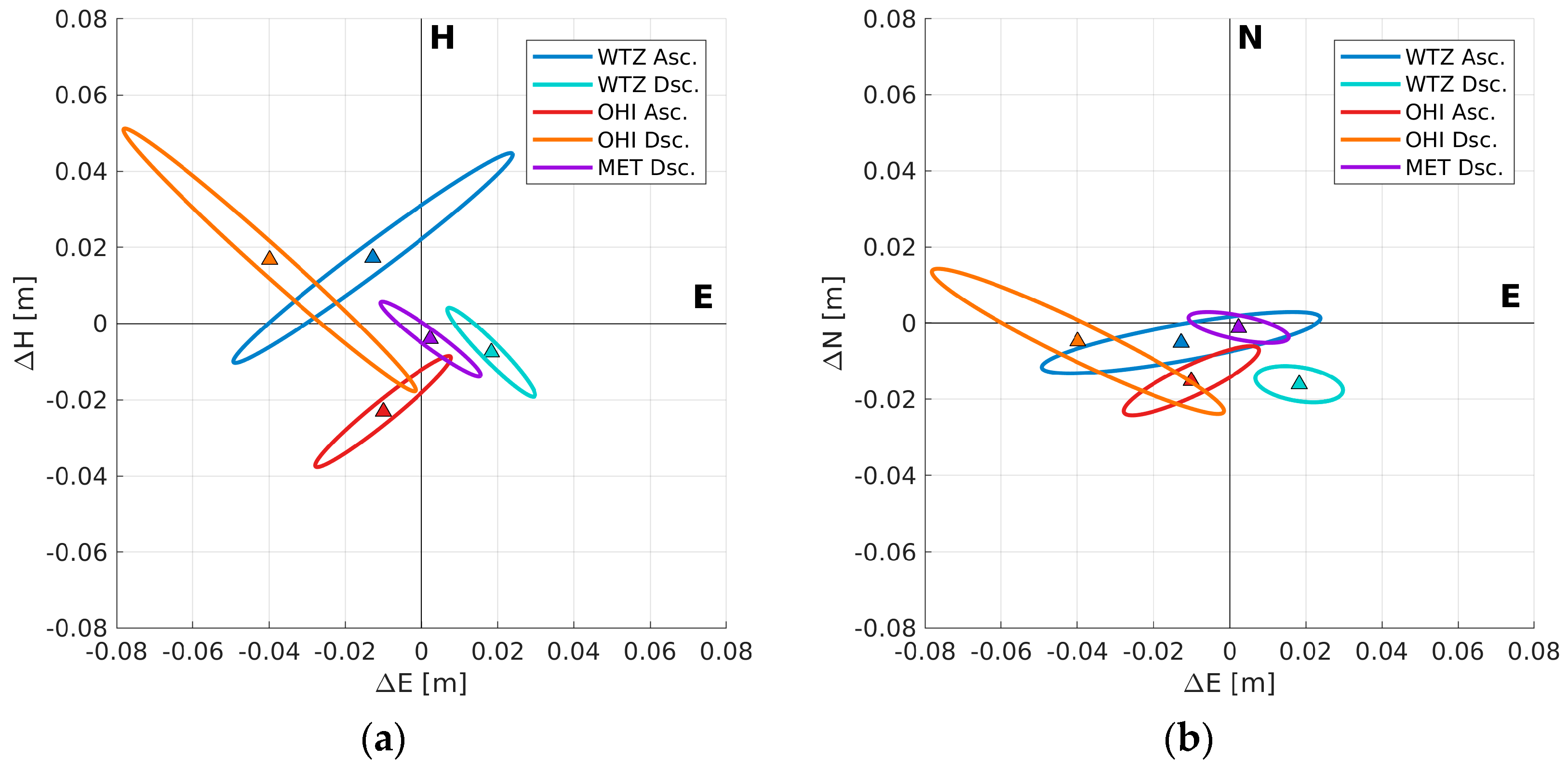
Another interesting aspect is the overall error distribution of the coordinate solution, namely the error ellipsoid, which is visualized in
Figure 9. Because of the same scaling for a confidence level of 95%, the horizontal and vertical cross sections shown in the graphics directly correspond to the confidence values listed in
Table 7. The
,
,
are simply the bounding boxes of the ellipses, while the smallest errors are found to be in the range direction, see
Figure 9a. All the ellipses are inclined to about 40 degrees, which is the average incidence angles of the passes for the individual CRs, see the angles listed in
Table 5. As expected, the underlying intersection geometries are most sensitive in the SAR range direction, and least sensitive in the perpendicular cross-range direction. The horizontal view, see
Figure 9b, has a similar behavior, but here it is the azimuth that dominates the orientation. The smaller axes coincide with the local sensor heading, which is nearly north-south due to the sun-synchronous orbit used by TerraSAR-X [
29]. Only towards the polar regions, the tracks start to converge, leading to the slightly more tilted horizontal error ellipses of the CRs at GARS O’Higgins. Therefore, the azimuth is almost only sensitive for the north-south component. These error patterns also explain the different confidence levels derived for local north, east and height (
Table 5), and they make it immediately clear, why the ideal setup for the application of SAR positioning is a reflector with a common phase center for ascending and descending passes. This concept was already studied with TerraSAR-X in a small experiment at Wettzell [
30].
In summary, the 3-D localization experiments underline the very high absolute accuracy that can be achieved with absolute SAR positioning under ideal circumstances. Moreover, they confirm the performance of our positioning method, the high quality TerraSAR-X radar payloads, the fidelity of the SAR processing, as well as the accuracy of the annotated orbit product.


