Microphytobenthos Biomass and Diversity Mapping at Different Spatial Scales with a Hyperspectral Optical Model

Abstract

This work is an extension of the MicroPhytoBenthos Optical Model (MPBOM) workflow. The model was based on the observation that the biofilm itself has a negligible inherent reflectance and can be described solely by the ratio between its apparent reflectance (R_A) and background reflectance (R_B), allowing a straightforward calculation of the absorption coefficient (α). This coefficient is directly related to pigment concentrations estimated by High Performance Liquid Chromatography (HPLC). To run the model, assess and extend the use of α, the background contribution is a critical step. This work shows that: (i) indices based on reflectance and absorption coefficient spectra derived from the optical model correctly identified the main microphytobenthos (MPB) groups covering a pixel; (ii) contrary to the R_A index each new α index was insensitive to biomass variations; (iii) for each MPB group there was a significant linear relation between the biomass estimated by HPLC and α peak at 673 nm; (iv) indices based on α spectra were almost insensitive to mixing constraints at a subpixel level. Knowing the background reflectance contribution of MPB biofilms, α can therefore be used to map MPB algal composition and biomass at any scale from MPB synthetized in laboratory to intertidal mudflat airborne observations.

1. Introduction

Coastal intertidal mudflats are highly productive ecosystems partially due to the presence of microphytobenthos (MPB) assemblages living at the sediment surface [1]. MPB primary production can represent a significant part of the total primary production in tidal systems [2]. MPB is mainly dominated by diatoms [3], but other groups can be found such as euglenids, chlorophytes (green algae), cyanobacteria, dinoflagellates [3,4] and could be mixed with rhodophyta spores and propagules [5]. Diatoms belong to a class of microalgae known for their richness in carotenoid pigments [6] giving a golden-brown color characteristic at the sediment surface and forming dense biofilms in the first millimeters of mudflat sediment. Motile diatoms (epipelic, mud-dwelling) typically form these biofilms only during low tide periods showing movement synchronization with tidal periods [3,7,8]. The cohesion between cells in a biofilm comes from the secretion of exopolysaccharides (EPS) recognized as agents for the biogenic stabilization of sediment [9,10]. However, this cohesion does not completely prevent MPB assemblages from being resuspended by tidal currents [10,11], which can represent a significant food source for suspension-feeders and benthic invertebrates [12,13,14] or wading birds [15].

MPB large-scale assessments are needed to estimate its contribution at an ecosystem level [16]. Currently, only remote sensing techniques can provide synoptic information while saving time-consuming extensive field sampling campaigns to quantify MPB biomass spatial distribution [17]. When mapped with multispectral sensors, biomass is usually expressed in NDVI (Normalized Differential Vegetation Index, [18]) products [19,20,21,22]. However, hyperspectral resolution allows exploitation of the full shape of continuous reflectance spectra and analysis of narrow absorption band characteristics of different MPB groups [23,24]. To improve MPB mapping based on empirical approaches, Kazemipour et al. [25] used hyperspectral data to develop a robust model allowing the retrieval of the MPB optical properties, by considering a biofilm as a homogenous compact layer of translucent microalgal cells with two plane-parallel faces over various opaque backgrounds (mud, sand, Spectralon^® panel). Consequently, all MPB embedded in the sediment, below the opaque surface are not quantified. They demonstrated that the inherent MPB reflectance was negligible and that the non-absorbed light passing through the cell layer is reflected only by the background. The model called MPBOM (MicroPhytobenthos Optical Model) was used to retrieve the biofilm absorption coefficient (α), which was linearly related to biomass concentrations estimated by independent chromatographic analyses measuring the same physical variable α. The difference between these two set of α measurements comes from the fact that High Performance Liquid Chromatography (HPLC) quantified one after the other isolated pigments extracted in organic solvants whereas hyperspectral spectra quantified pigments mixed in living cells stacked in various thickness of biofilms. Whatever the techniques used, the same physical variables is measured and thus without any background effect which must be removed to insure the physical link with α. In this work, we reorganized the model workflow to make it more comprehensible and to demonstrate that α values are easily obtained since they are only dependent on two reflectance measurements corresponding to (i) the apparent reflectance of the MPB on its background and (ii) the reflectance of the background alone. Note that [26] study also removed the background assimilated to a trend like [23,24]. By subtracting this trend in logarithm of reflectance they basically divided each spectrum by its background, but working with logarithmic values they calculated an index which may be equivalent to an absorbance values, like also [27] did from transmittance. This should not be confused with the absorption coefficient. The full comparison with alternative methods would require intercalibrations beyond the scope of this work.

All photosynthetic organisms, including MPB possess the ubiquitous chlorophyll-a (Chl a) pigment, which is remotely sensed by its wide absorption in the red domain, around 670 nm. However, by analyzing this absorption band alone in vivo without pigment separation like HPLC, it is not possible to distinguish the diversity of vegetation. Although the distinction between MPB and macrophyte is commonly done using NDVI thresholds, it is not possible to differentiate the main groups within the MPB assemblage [19,21]. Only hyperspectral data allow this distinction, based on specific absorption bands due to pigment fingerprints: Chl c and fucoxanthin for diatoms, Chl b for euglenids and chlorophytes, phycocyanin and phycoerythrin respectively for cyanobacteria and rhodophytes [28,29]. For instance, [24,30] introduced new spectral indices: MPBI (MPB Index), I_Diatom (Index of Diatom) and I_Euglenid (Index of Euglenid), respectively to distinguish MPB from macrophytes, and to further distinguish diatoms from euglenids. The present study also completes this set of indices to discriminate cyanobacteria and rhodophytes within MPB with two new indices: I_{Cyanobacteria} (Index of cyanobacteria) and I_Rhodophytes (Index of Rhodophyte).

Patchiness is an inherent characteristic of MPB biofilms [31]. MPB patches can exhibit high spatial variation on scales ranging from mm to km [23,32] leading to mixed pixel problems. Combe et al. [23] showed that MPB was characterized by patches of various biomasses laying on various background next to each other forming a unique reflectance spectrum per combination of translucent intimate mixing of MPB biomasses and simple mixing of backgrounds. Combe et al. [23] used the unicity of this reflectance to map such non-linear mixing of MPB and background with a comparison to a simulation of all possible combinations. Kazemipour et al. [24,25] partially solved this issue with the MPBOM by the separation between translucent MPB absorption coefficient and opaque background reflectance. This work developed the MPBOM with new equations defining the imbrication of translucent intimate mixture of biofilms at the surface of opaque simple mixture of backgrounds occurring when aggregating millimeter-level pixels as sub-pixels within centimeter-level to meter-level pixels. A set of applications ranging from laboratory experiments, allowing direct HPLC calibration, to field observations at an intermediate metric scale are used to discuss sub-pixel aggregation and field sampling. Two contrasting intertidal sites with different sediments (muddy vs. sandy) were imaged from airborne platform and provided macroscale datasets to test background composition variations. Diversity and biomass maps presented in this study illustrate the efficiency of the new MPBOM workflow as a powerful tool available for ecological studies of intertidal microphytobenthos biofilms.

2. Materials and Methods

2.1. Hyperspectral Measurements and Image Processing

All laboratory measurements were carried out using a standard HySpex VNIR 1600 camera from Norsk Elektro Optikk, Skedsmokorset, Norway, with a 4.5 nm spectral resolution in 160 channels, sampling the signal every 3.6 nm between 400 nm and 1000 nm and calibrated in radiance in a row of 1600 pixels. This camera was set on a frame in the laboratory above a scanning plate that moved the samples in synchronization with the detector integration time and a noise reduction procedure averaging 10 acquisitions per line. An airborne HySpex VNIR 1600 camera was used for airborne and ground image acquisitions. In the field, it was mounted on a rotating stage grabbing a panorama image with incident angles from 0° to 45°. Inside the Chieftain PA31-350 aircraft, from PIPER, Vero Beach, Florida, United States, the camera was mounted on the floor in front of a glassless window and it was synchronized with global positioning system (GPS) time. Airborne campaigns were carried out with the cooperation of GEOFIT and PIXAIR companies and the LiDAR platform of Nantes-Rennes universities for its positioning system only. Flight conditions were chosen to maximize the spatial resolution at 0.7 m per pixel.

Laboratory and ground measurements were calibrated with synchronous Spectralon^® measurements. Reflectance was calculated as the ratio between the target radiance and the white Spectralon^® reference. Laboratory measurements used light from quartz halogen lamps plugged into a controlled power supply giving an accurate smooth irradiant spectrum between 500 nm and 2500 nm. In the field, conditions were optimum (a sunny day) maximizing the light flux (minimizing the noise of the detector) and avoiding water vapor absorption enlargements in the near infrared (NIR). An equalizing filter, preventing the detector saturation, optimized the quality of the data between 400 nm and 1000 nm. Laboratory and airborne measurements were ground controlled using additional measurements with an ASD FieldSpec3 FR spectrometer from Malvern Panalytical Ltd, Royston, UK. Spectral data were calibrated in radiance from 300 nm to 2500 nm and sampled every 1 nm for an effective spectral resolution of 4 nm in the visible near infrared (VNIR) and 10 nm in the short wavelength infrared (SWIR) region.

Airborne images were calibrated using daylight atmospheric corrections completed with geometric corrections. The record of the aircraft attitude, using a fast inertia measurement unit (IMU) coupled to an accurate GPS, allowed the calculation of a trajectory which was provided by GEOFIT for this study. PARGE software version 3.4 [33] was used to project the image in the geographic coordinate system. Data were subsequently processed with Atmospheric and Topographic Correction for Airborne Scanner Data (ATCOR 4) version 7.2 [33], which used the initial image geometry to better take into account the properties of the camera. It used the MODTRAN 5 atmospheric model for estimating the water vapor content in each pixel, taking into account the aerosol diffusion effects and the spectral noise level of the dark reference of each image (see [33]). The water vapor estimation was done at 820 nm and the atmosphere model used was maritime.

Noise reduction in the laboratory was done by averaging 10 to 20 acquisitions for each line. Noise of all images was also reduced by applying Minimum Noise Fraction (MNF) transformations [34,35]. MNF could not however remove all noise from the images and some channels/bands had to be interpolated with their neighbors to optimize MNF outputs.

A final adjustment on a bright target was also carried out to remove any final effects of degradation of camera sensitivity calibrations that with time produced a constant artifact all over the images, which could not be statistically identified by the MNF procedure. This bright target adjustment was a minor correction of the gain, but it facilitated the comparison between data acquired at different scales.

2.2. Laboratory Experimentations

All laboratory MPB biofilms were prepared following the protocols of [21,25] to have access to the true optical properties of the biofilms. Biofilms of the diatom Entomoneis paludosa (NCC 18 from the Nantes Culture Collection, MMS Laboratory, Nantes, France) and the euglenid Euglena gracilis (CCAP 1224/5 from the Culture Collection of Algae and Protozoa, Dunstaffnage Marine Laboratory, Oban, UK) were prepared by slowly filtering different dilutions from monospecific cultures on polycarbonate filters [21,25]. Spectral measurements were performed immediately after filtration with a nadir looking camera. The camera was set in laboratory conditions to scan successively 99% Spectralon^® reference plate and samples with square pixels providing a spatial resolution of about 0.2 mm per pixel. The reflectance was obtained by dividing each column of the image by the mean intensity of the Spectralon^® (~99% reflectance in the VNIR range, so conversion to absolute reflectance was not necessary). All measurements were done on 99%, 50% and 20% Spectralon^®, with each Spectralon^® positioned under glass Petri dishes containing filters and with 3 different backgrounds (Figure 1). Samples were then kept frozen (−80 °C) until pigment analysis by HPLC, used in order to separate, identify and quantify all pigments. The protocol for pigment extraction, HPLC equipment and the elution program are detailed in [21]. HPLC basically analyses the absorption coefficient allowing to link the corresponding reflectance spectrum to the pigment composition as described in [21] and to directly connect both absorption coefficients from [25]. Chlorophylls and carotenoids were detected and characterized by their absorption spectra in the visible range of wavelengths. Pigment concentration values were determined from absorption at 440 nm following an external calibration using pigment standards (DHI LAB Products, Denmark). Pigment content was reported in relation to surface area and expressed as mg m⁻². In case of chlorophyll a (Chl a) this content is given in mg Chl a·m⁻². Biofilms on filters were also measured with the ASD spectroradiometer to obtain comparable data with spectral libraries obtained by [28,29], with other groups of MPB. Spectra of cyanobacteria (Spirulina platensis) and a unicellular rhodophyta (Porphyridium cruentum) from these previous works were added to the analysis.

2.3. Ground and Airborne Field Studies

2.3.1. Muddy Site

Bourgneuf Bay (French Atlantic coast), located south of the Loire estuary was chosen as the muddy site (46–47° N, 1–2° W, Figure 2a). It is a macro tidal bay with a maximum tidal amplitude of 6 m during spring tides with an intertidal mudflat (340 km²) partly occupied by large oyster farms (about 10%) and less mussel. Wild oysters are also abundant on rock outcrops. The mudflat regularly displays superficial MPB biofilms at low tide that can be detected with remote sensing imagery [21] with a complex relationship to sediments and oyster farms characterized by strong gradients behind the scope of this methodologic work. As with other estuarine bays, MPB contributes to the food web as a significant primary producer (e.g., [36]).

The eastern part of the bay was imaged on 17 October 2016 during low tide between 10:10 and 11:08 UT (Figure 2a). The maximum sun elevation was around 35° and the HySpex camera was mounted in the PA31 aircraft from PIXAIR.

To investigate an intermediate scale between the laboratory and the entire mudflat, a ~4 m panorama was acquired in situ on 7 July 2016 at 10:58 UT using the HySpex VNIR camera on a rotating stage at the “La Coupelasse” site (47°00′57” N, 2°01′27” W, Figure 2c). The inclination was close to 45° with a sun elevation of 63° coming from south-east on the back and right of the image which provided ~0.2 mm per ~0.5 mm pixels in x and y directions of the area of interest (Figure 2c). A Spectralon^® parallel to the image plane on the left was used for reflectance calculation.

2.3.2. Sandy Site

The Authie estuary was chosen as the sandy site (50°22′25” N, 1°37′52” E, Figure 2b). It is located on the French coast of the Eastern English Channel (EEC), and is characterized by a semi-diurnal macro tides. The Authie estuary forms a shallow elongated embayment that shows a rapid infilling of sand from the English Channel [37,38]. Morphologically, this estuary is considered as an “estuarine back-barrier” type [39]. Along the marine side, the morphology is marked by the presence of ridges and runnels which are particular characteristics of the EEC macro tidal coast system. Upper and middle parts of the estuary are mainly composed by intertidal sandflats and sand bars ranging from fine to medium in size (D₅₀ = 0.1–0.6 mm) including a shelly debris component. The lower estuary is mainly composed of silty sediment. Mudflats and salt marches only appear in the inner estuary [40] where MPB, mainly diatoms, can form biofilm patches. Unlike Bourgneuf bay, Authie estuary is not an extensive aquaculture site. The MPB of this estuary was first studied by Carrère et al. [41]. This sandy site was imaged on 21 July 2016 between 9:07 and 09:58 (UTC) with the same flight conditions and camera settings as in the Bourgneuf bay site (Figure 2b). The maximum sun elevation was around 49°.

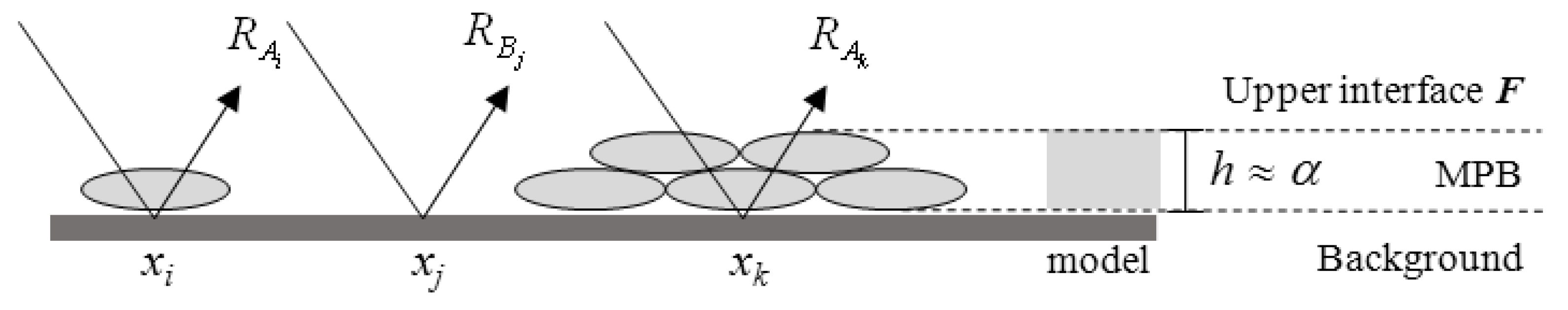
2.4. The MicroPhytoBenthos Optical Model

2.4.1. Optical Properties

The microphytobenthos optical model (MPBOM) defined by Kazemipour et al. [25] considers that a microphytobenthic biofilm is a homogenous compact layer having two rough plane-parallel faces, deposited on a background (Figure 3). Light travels twice through the biofilm, forward and backward, after reflection on a background. This round-trip of light through a translucent biofilm after reflection on an opaque background is a key optical property of the model. The biomass of the homogeneous MPB cell layer is estimated with the absorption coefficient (α), which is directly proportional to the height (h) of the layer (Figure 3), and to the number of cells per surface unit which can be estimated in mg Chl a·m⁻².

Considering that the attenuation coefficient increases by stacking diatom cells tens µm in thickness, which are not measurable individually, following [25,42] we can assimilate h to α. Lambert’s law of absorption can therefore be rearranged to give Equation (1), where η is the biofilm attenuation coefficient:

$$\eta =e^{-\alpha h}\stackrel{\alpha h=\alpha }{\to }\alpha =-\ln (\eta )$$

(1)

The first step of the model consists in estimating the biofilm inherent reflectance R and transmittance T from apparent reflectance R_A, which is the measure commonly performed with a spectroradiometer or a hyperspectral imager. R and T are retrieved considering a bright (R_B1) and a dark (R_B2) background reflectance (see Equations (5) and (6) in [25]).

$$R=\frac{R_{A1}{R}_{B2}-R_{A2}{R}_{B1}}{R_{B2}-R_{B1}-R_{B1}{R}_{B2}(R_{A2}-R_{A1})},$$

(2)

$$T={\left[\frac{\left(R_{A1}-R\right)\left(1-R{R}_{B1}\right)}{R_{B1}}\right]}^{0.5}={\left[\frac{\left(R_{A2}-R\right)\left(1-R{R}_{B2}\right)}{R_{B2}}\right]}^{0.5},$$

(3)

The application of the MPBOM to a biofilm composed of another group of diatoms used to build this model requires that R is negligible and invariant while T varies as a direct function of biomass. Verification that the biofilm R is negligible can be established by a simple measurement on white and black backgrounds as shown in Figure 1. It is a prerequisite to use the model for the different groups of MPB constituting a biofilm. The calculated inherent reflectance and transmittance spectra are then related to the attenuation coefficient, η, and interface reflectance and transmittance, R_F and T_F (Figure 3, Equations (3) and (4) and Figure 6-b in [25]).

$$R=R_F+\frac{R_F{T}_F^2{\eta }^2}{1-R_F^2{\eta }^2},$$

(4)

$$T=\frac{T_F^2\eta }{1-R_F^2{\eta }^2},$$

(5)

Kazemipour et al. [25] used this iterative method of [43] to estimate η from R and T by a loop between Equations (6), (7) and Equation (8) being initialized to 1.

$$R_F=\frac{R}{1+\eta .T},$$

(6)

$$T_F={\left[\frac{(1-{\eta }^2.R_F^2).T}{\eta }\right]}^{0.5},$$

(7)

$$\eta =R_F+T_F,$$

(8)

Kazemipour et al. [24] subsequently avoided the iterative step, considering that the biofilm inherent reflectance was negligible (R = R_F = 0) and proposed the following simplifications:

The transmittance (T) of Equation (5) can be estimated from Equation (3) with measured reflectance spectrum of the pixel (R_A) and the reflectance spectrum of the substrate (R_B)

$$T^2=\frac{\left(R_A-R\right)\left(1-R.R_B\right)}{R_B}\stackrel{R\approx 0}{\to }T=\sqrt{\frac{R_A}{R_B}},$$

(9)

The interface transmittance (T_F) of Equation (7) becomes:

$$T_F={\left[\frac{(1-{\eta }^2.R_F^2).T}{\eta }\right]}^{0.5}\stackrel{R_F\approx 0}{\to }{T}_F=\sqrt{\frac{T}{\eta }},$$

(10)

The iterative condition of Equation (8) becomes:

$$\eta =R_F+T_F\stackrel{R_F\approx 0}{\to }\eta =T_F,$$

(11)

Then a combination of Equations (10) and (11) gives a straight correspondence between η and T

$$\eta =\sqrt{\frac{T}{\eta }}\hspace{1em}\mathrm{or}\hspace{1em}{\eta }^3=T,$$

(12)

The absorption coefficient (α) can now be calculated from η by combining Equations (1), (9) and (12):

$$\alpha =-\ln \left(\eta \right)\stackrel{R\approx 0}{\to }\alpha =-\ln \left(\sqrt[3]{T}\right)=-\ln \left(\sqrt[6]{\frac{R_A}{R_B}}\right),$$

(13)

And conversely we have:

$$\frac{R_A}{R_B}=\exp {\left(-\alpha \right)}^6,$$

(14)

By rearranging this new Equation (14) it is then possible to simulate in a pixel the apparent reflectance (R_Amn) of m MPB concentrations intimate (α) mixing over any simple (R_B) mixing of n background with the second new Equation (15):

$$R_{A_{mn}}=\left({\displaystyle \sum _{j=1}^n{R}_{B_j}}\right)\cdot \exp {\left(-{\displaystyle \sum _{i=1}^m{\alpha }_i}\right)}^6,$$

(15)

Equation (15) calculating separately α and R_B mixing, prior the calculation of apparent reflectance, is the major contribution of this work and the following Equation (16) calculating the apparent reflectance (R_Ai) of a biofilm over another background (R_Bi) is a validation of empirical calculations used in previous works.

$$R_{Ai}=R_{Bi}\cdot \frac{R_A}{R_B},$$

(16)

2.4.2. Background Estimation

It is not possible to directly measure background reflectance in the field. However, [25] showed that biofilms have a 100% transmittance spectral window between 750 nm and 920 nm giving access to the optical properties of the background. This peculiarity, inherent to a MPB biofilm, can be used for R_B estimation. When the background reflectance spectrum is known, it may not have the same exposure and an adjustment of its intensity in the 750–920 nm spectral windows (Equation (17)) avoids artifacts of calculation when variable irradiance conditions locally decrease the apparent reflectance.

$$R_{Bj}=R_{Bi}\cdot \frac{{\displaystyle \sum _{\lambda =750}^{920}{R}_{B_j}}}{{\displaystyle \sum _{\lambda =750}^{920}{R}_{B_i}}},$$

(17)

When the background reflectance is unknown, a regression line of R_A in the 750–920 nm range, giving a slope and intercept, can simulate a straight line background R_Bs over the full spectral range (400–1000 nm) as shown in Figure 4. Such background simulation imply however that sediment display neutral spectra, such as a sandy beach (Figure 4), at least in the 550–750 nm range are required for the unbiased measurement of pigment absorptions. Some sediment contains shell debris of mollusks or barnacles presenting a large absorption ending at 850 nm (Figure 4). In crustaceans, this is due to the complex organic matrix embedding the pure calcite component of its viscoelastic shell [44]. Thus, the background loses its neutral aspect and its simulation displays a steep slope cutting its own reflectance in the visible domain, which can bias the pigment absorption estimation. When a sediment surface is covered by water layers, like puddles (Figure 4), water absorption features can inverse the slope of the regression line of background simulation, which gives an aberrant absorption coefficient. Therefore, the MPBOM model is not applicable for the following two conditions (i) if the background regression line is intersecting the visible domain because of non-neutral reflectance due to particular sedimentary compositions; (ii) if there is strong negative slope due to the presence of a water layer.

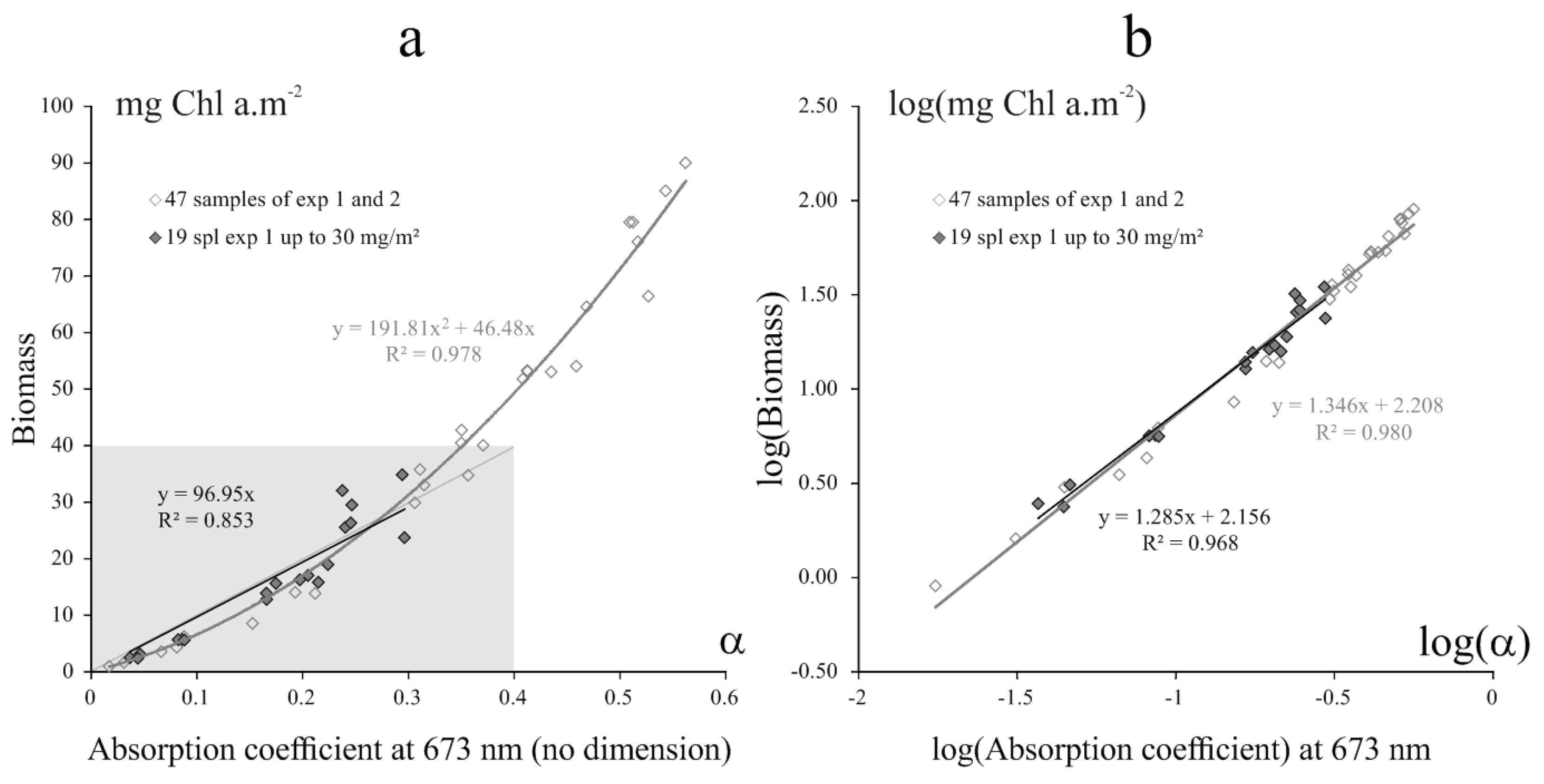
2.4.3. Biomass Estimation

The absorption coefficient is the result of an overlay of separate pigment absorptions in the 400–700 nm wavelength range and is therefore highly influenced by MPB biomass variations. As the absorption coefficient presents a very distinct peak at 673 nm, [25] used this feature to obtain isometric linear regressions relating to biomass, using chlorophyll a (Chl a) as a proxy, measured with HPLC with absorption coefficient values at 673 nm. For the range values of α from 0 to 0.4 (grey area Figure 5a), corresponding to biomass below 40 mg Chl a·m^-2, commonly found in both sites tested in this work, the relationship with Chl a was linear (Equation (18)) with a the slope of the regression used to convert absorption coefficient peak at 673 nm in biomass of the analyzed MPB type.

$$Biomass(\mathrm{mg}\mathrm{Chl}\mathrm{a}\cdot {\mathrm{m}}^{-2})=a\cdot {\alpha }_{673\mathrm{nm}},$$

(18)

For α values up to 0.4, the relationship was not still linear due to a lesser absorption efficiency by the Chl a in the cell layers. This deviation was due to the package effect increasing with biomass, but also to physiological responses of microalgae to light conditions during the experimentation [26,29,45]. To overcome this deviation, [46] suggested the use of a log-log plot (Figure 5b). It gave a better regression line as shown by [26] with plus or minus a scale factor of intercalibration. But the use of an arithmetic plot, as we suggested, allowed this deviation detection (Figure 5a) which is potentially useful in MPB monitoring status health.

To apply this relationship to different MPB groups, the prerequisite is that each group must have been previously identified using specific shapes of reflectance/absorption coefficient spectra.

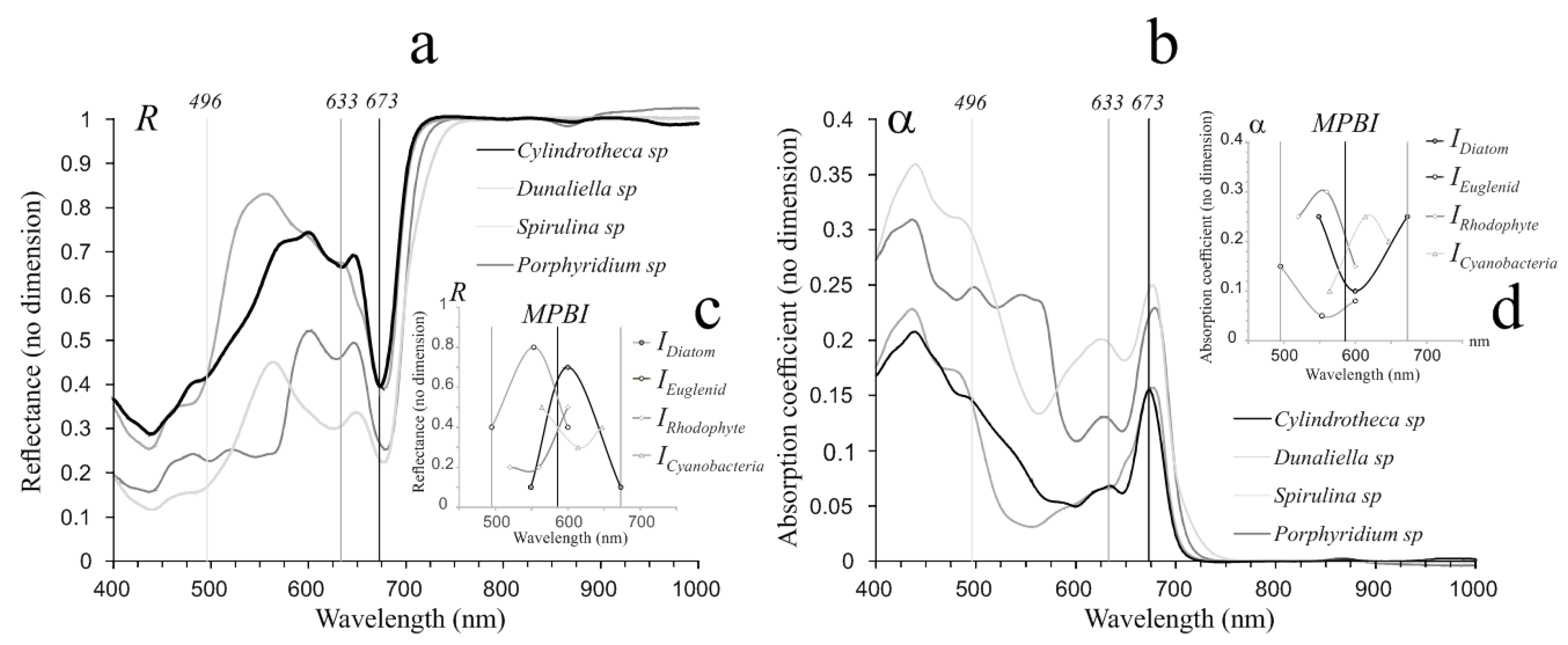
2.4.4. MPB Groups Identification by R and α Spectral Indices

The analysis of the R shape was used by [24] for the identification of the main groups of MPB reflectance indices. This work extends the analysis to α spectra and adds two new spectral indices for cyanobacteria and red microalgae such as rhodophyta (

Table 1. Spectral indices used in the new MPBOM workflow to identify the type of biofilm: diatom, euglenid, cyanobacteria or rhodophyte. Indices used narrow bands of reflectance (left column) and of absorption coefficient α (right column). All indices are new, except NDVI_HR, I_Diatom and I_Euglenid from [24] and MBPI from [30].

Reflectance R	Absorption Coefficient α
$NDV{I}_{HR}=\frac{R_{800}-R_{673}}{R_{800}+R_{673}}$	$NDVI{\alpha }_{HR}=\frac{R_{673}-R_{800}}{R_{673}+R_{800}}$
$MPBI=\frac{2\times R_{586}}{R_{495}+R_{673}}-1$	$MPBI\alpha =\frac{{\alpha }_{495}+{\alpha }_{673}}{2\times {\alpha }_{586}}-1$
$I_{Diatom}=\frac{2\times R_{600}}{R_{549}+R_{673}}-1$	$I{\alpha }_{Diatom}=\frac{{\alpha }_{549}+{\alpha }_{673}}{2\times {\alpha }_{600}}-1$
$I_{Euglenid}=\frac{2\times R_{553}}{R_{600}+R_{495}}-1$	$I{\alpha }_{Euglenid}=\frac{{\alpha }_{600}+{\alpha }_{495}}{2\times {\alpha }_{553}}-1$
$I_{Cyanobacteria}=\frac{R_{564}+R_{647}}{2\times R_{614}}-1$	$I{\alpha }_{Cyanobacteria}=\frac{2\times {\alpha }_{614}}{{\alpha }_{564}+{\alpha }_{647}}-1$
$I_{Rhodophyte}=\frac{R_{520}+R_{600}}{2\times R_{560}}-1$	$I{\alpha }_{Rhodophyte}=\frac{2\times R_{560}}{R_{520}+R_{600}}-1$
$I_{ClearWater}=\frac{2\times R_{812}}{R_{740}+R_{880}}-1$

). Euglenids and chlorophytes (green algae) having the same pigment composition could not be separated.

The purpose of each index is to measure, in a short wavelength interval (Figure 6c,d), the positive and negative curvature of a smooth continuous spectrum forming a characteristic arc of a particular combination of pigments. This can be done by calculating the ratio between the center and borders of the spectral well and peak, as in the spectral shape analysis method of [47] equivalent to the Narrow/Wide band ratio of [48]. Each index was also designed to measure the increasing height of peaks and wells, so negative values were set at zero.

NDVI, a two band index, was calculated with HySpex high resolution (NDVI_HR, R column, Table 1) and all other reflectance indices were calculated with three bands, analyzing the characteristic curvature of reflectance spectra formed by particular associations of pigments (Figure 6c). The MPBI index proposed by [30] was used to discriminate MPB from macrophytes (macro algae and seagrass).

NDVI_HR was used in the first step for the selection of the vegetation areas. We used an empirical threshold at 0.1, calculated with sand reflectance without any VNIR absorption, but adjustments were possible according to specific case studies (for instance 0.15 at the Bourgneuf site). Secondly (with NDVI_HR > 0.1) all reflectance data with MBPI greater than NDVI_HR was identified as MPB. The MPB type was then defined in the third step, which was based on the ranking between the indices shown in

Table 2. MPB main group spectral self-identification using indices calculated on reflectance data. Indices in brackets are set at 0.

MPB threshold	If (NDVIHR > 0.1 and MPBI > NDVIHR)
Diatoms	MPBI > IDiatom > NDVIHR > 0 (IEuglenid, ICyanobacteria, IRhodophyte)
Euglena and green microalgae	MPBI > IEuglenid > NDVIHR > IDiatom ≥ ICyanobacteria ≥ 0 (IRhodophyte)
Cyanobacteria	MPBI > IEuglenid ≥ NDVIHR > ICyanobacteria ≥ 0 (IDiatom, IRhodophyte)
Rhodophyte and red microalgae	IDiatom > MPBI > IRhodophyte ≥ NDVIHR > 0 (ICyanobacteria, IEuglenid)

. The procedure classifies indices in descending order down to 0. It is a morphological analysis of reflectance spectra whatever their intensities. In order to correctly display the ranking between indices, we used the same lookup table [0, 1] for each index. By so doing, false colors in color composite images were proportional to the absolute indices ranking and can be used as a mixing detection. For instance, the combination of I_Diatom in red and I_Euglenid in green would display an orange false color for a mixing of 50% diatom and 50% euglenid whereas pure diatom appears red and pure euglenid appears green. We also introduced the I_ClearWater index for the detection of thin clear water layers over the mudflats when the negative slope of the background in the range 750–920 nm (Figure 4) did not permit the use of the optical model, whereas the interstitial water mixed within the sediment did not affect the spectrum shape between 400 and 900 nm.

All reflectance based indices were also calculated using the absorption coefficients (

Table 3. MPB main group type spectral self-identification using indices calculated on the absorption coefficient data. Indices between brackets are set at 0.

MPB threshold	If (NDVIHR > 0.1 and MPBI > NDVIHR) with NDVIαHR = 1
Diatoms	MPBIα > IαDiatom > IαEuglenid > IαCyanobacteria ≥ 0 (IαRrodophyte)
Euglena and green microalgae	MPBIα ≈ IαEuglenid > IαDiatom > IαCyanobacteria ≥ 0 (IαRhodophyte)
Cyanobacteria	MPBIα ≈ IαEuglenid > IαCyanobacteria> IαDiatom ≥ 0 (IαRhodophyte)
Rhodophyte and red microalgae	IαDiatom > MPBIα > IαRhodophyte ≥ 0 (IαEuglenid, IαCyanobacteria)

and Figure 6d). These absorption coefficient indices were only calculated for pixels identified as MPB using the reflectance criterion MPBI > NDVI_HR since NDVIα_HR = 1 for MPB while MPBIα can be lower than 1.

In practice, all these rankings were used to define imbricated masks. For example the vegetation mask embedding the MPB mask embedded itself in all diatom mask, euglenid mask, cyanobacteria mask and rhodophyte mask. This masking procedure based on rankings between indices, classifying each pixel on the basis of the most abundant MPB types, was necessary to present the biomass map through those masks with their corresponding indices of color composite images allowing the detection of any possible mixing or other effects that could modify the interpretation of the results.

3. Results

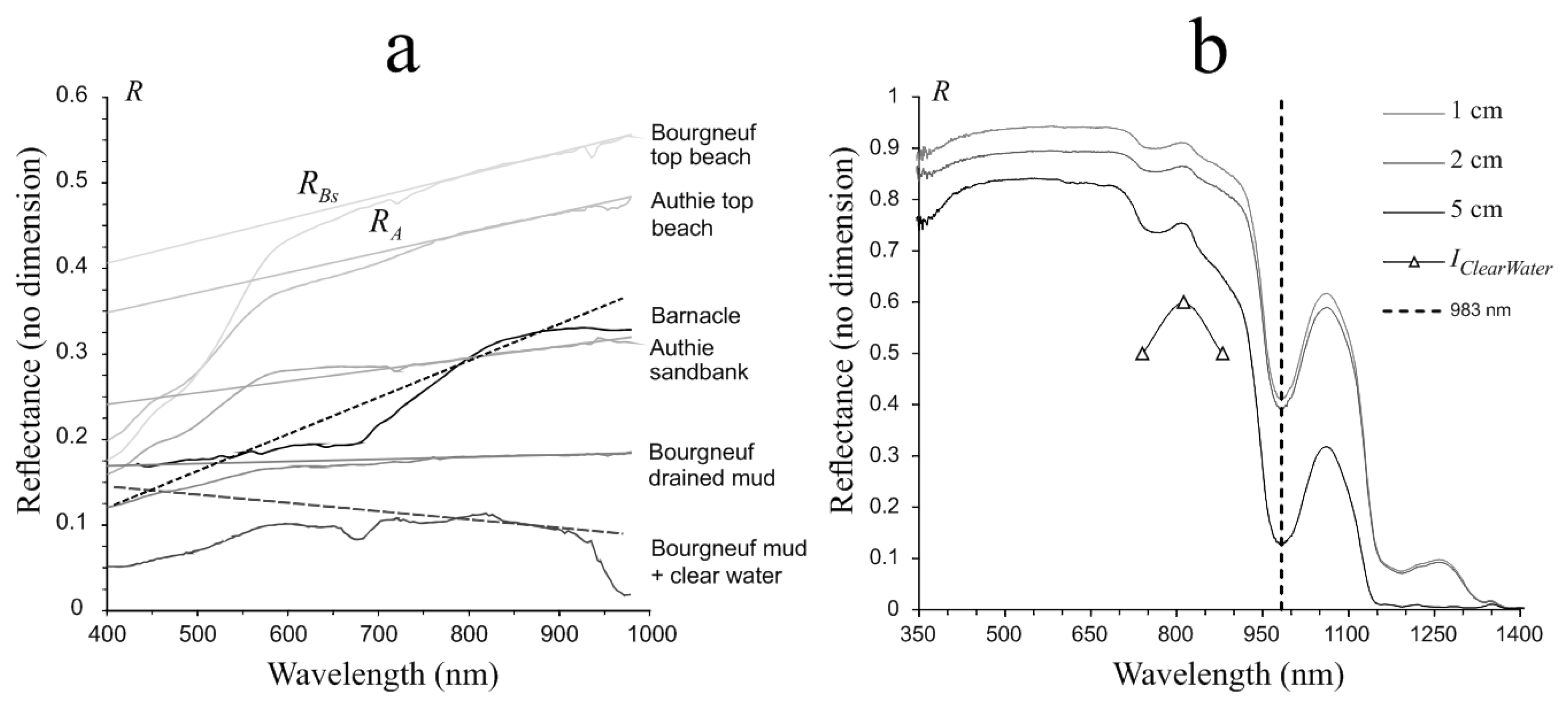
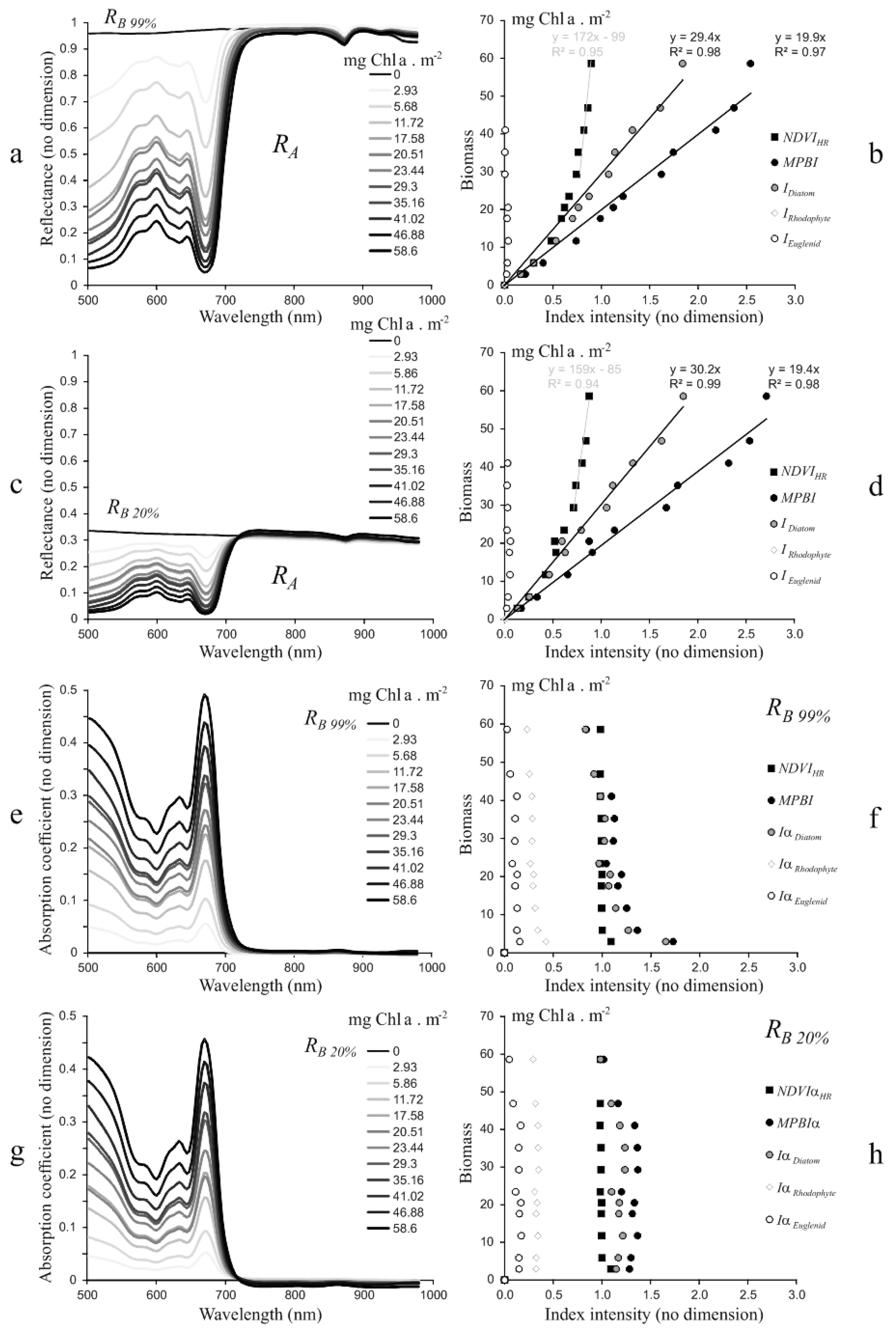
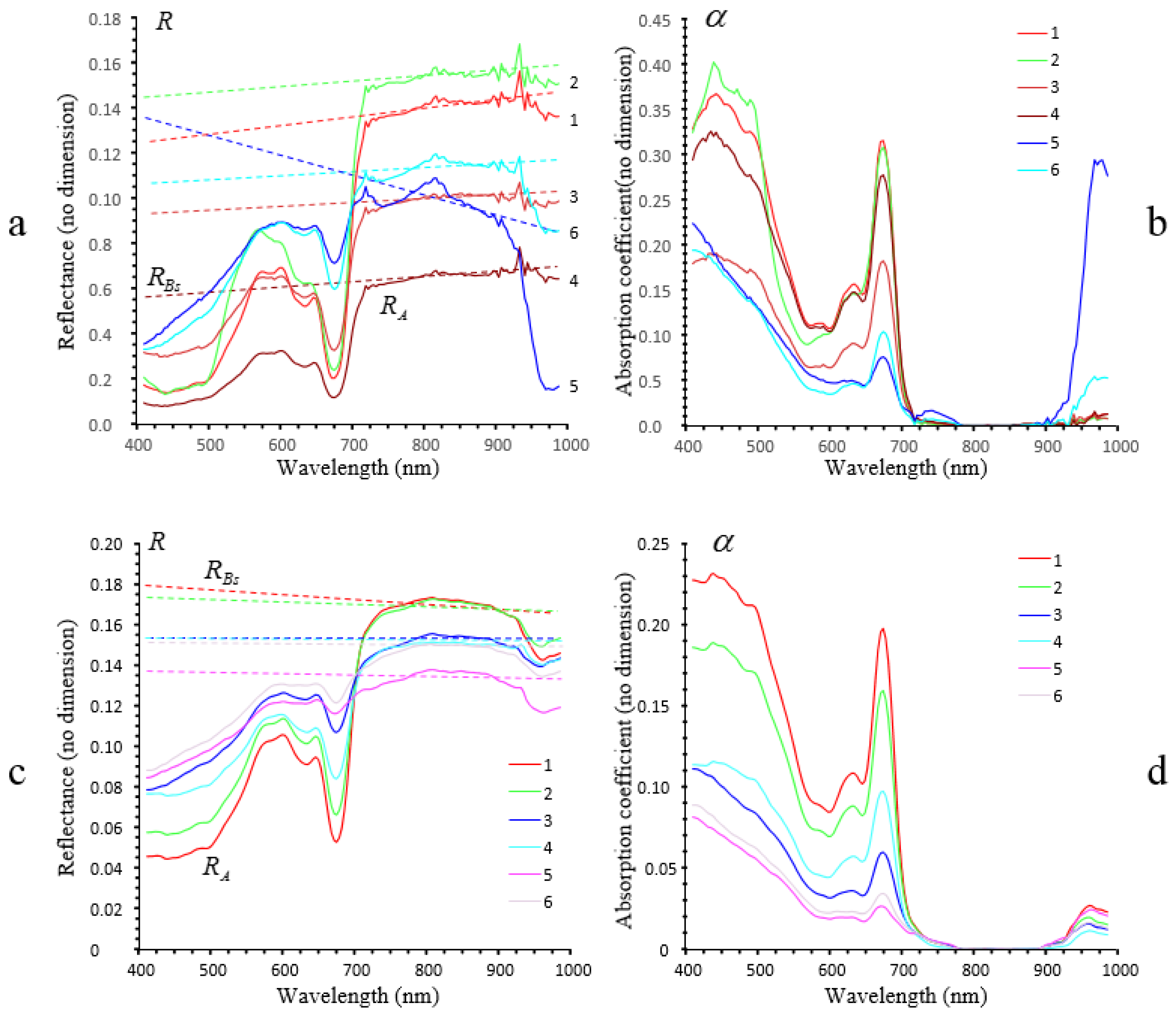
3.1. Spectra Analyses

Reflectance from the region of interest (ROI) were collected for each biofilm on wet filters of polycarbonate and their respective backgrounds on the HySpex image acquired in the laboratory (see Figure 1). Spectra were stored in a spectral library and used to build indices of spectral peak and well heights and estimate the biomass of each spectrum.

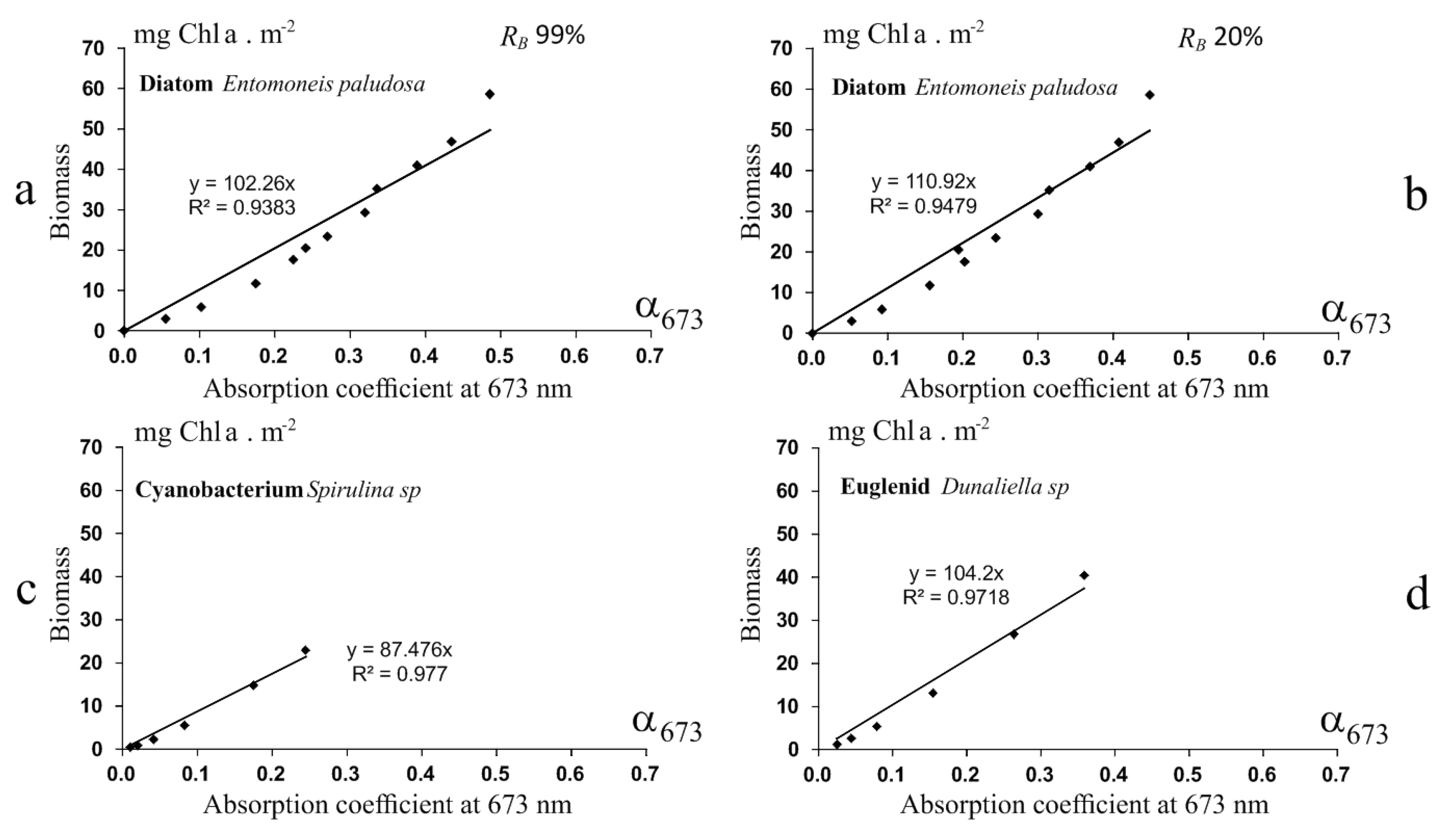
3.1.1. Biofilm Algal Composition and Biomass Estimation

Whatever is the biomass, diatoms R_A spectra displayed the same intensity in the 750–900 nm range for the 99% Spectralon^® background (Figure 7a) like for the 20% Spectralon^® background (Figure 7c) with absorption features related to biomass variations in the visible spectral range. According to the set of rules MPBI > I_Diatom > NDVI_HR > 0 (Table 2), biofilms were composed of diatoms (Figure 7b,d). Regardless of the background, the MPBI and I_Diatom indices presented the best relationship with biomass following regression line slopes of 20 and 29, respectively (Figure 7b,d). NDVI_HR showed an apparent saturation pattern for the highest biomass losing their correlation with biomass above 25 mg Chl a·m⁻² presenting a steep slope (159 and 172) and high intercept values (−85 and −99) of regression lines almost parallel to the biomass axis (Figure 6 b,d), while other indices I_Rhodophyte, I_Euglenid and I_{Cyanobacteria}, were null (Figure 7 b,d).

The absorption coefficient α displayed spectra which were independent of the background with intensity only changing with biomass variations (Figure 7e,g). All α indices were totally uncorrelated with biomass (almost parallel to the biomass axis) and displayed constant values (Figure 7f,h). Following Table 3 criteria, the ranking of MPBIα ≥ Iα_diatom (Figure 7f,h) indicated the correct presence of absorption coefficient spectra to the diatoms group. Small variations of MPBI and I_Diatom values were observed for biomass lower than 10 mg Chl a·m⁻² (Figure 6f). Relationships between the absorption coefficient spectra at 673 nm and biomass values estimated by HPLC were very strong with a coefficient determination of R² > 0.93 for each background (Figure 8). For other MPB groups, absorption coefficient spectra (not shown) were calculated from [28,29] spectral reflectance libraries based on monospecific cultures. Significant linear regressions were also observed between biomass and α₆₇₃ for cyanobacteria and euglenids with R² > 0.97 (Figure 7c,d). Contrary to R_A, for which all intensities and indices are correlated to the biomass, α allows separation of the information about the distribution of the pigments with indices from the biomass variation.

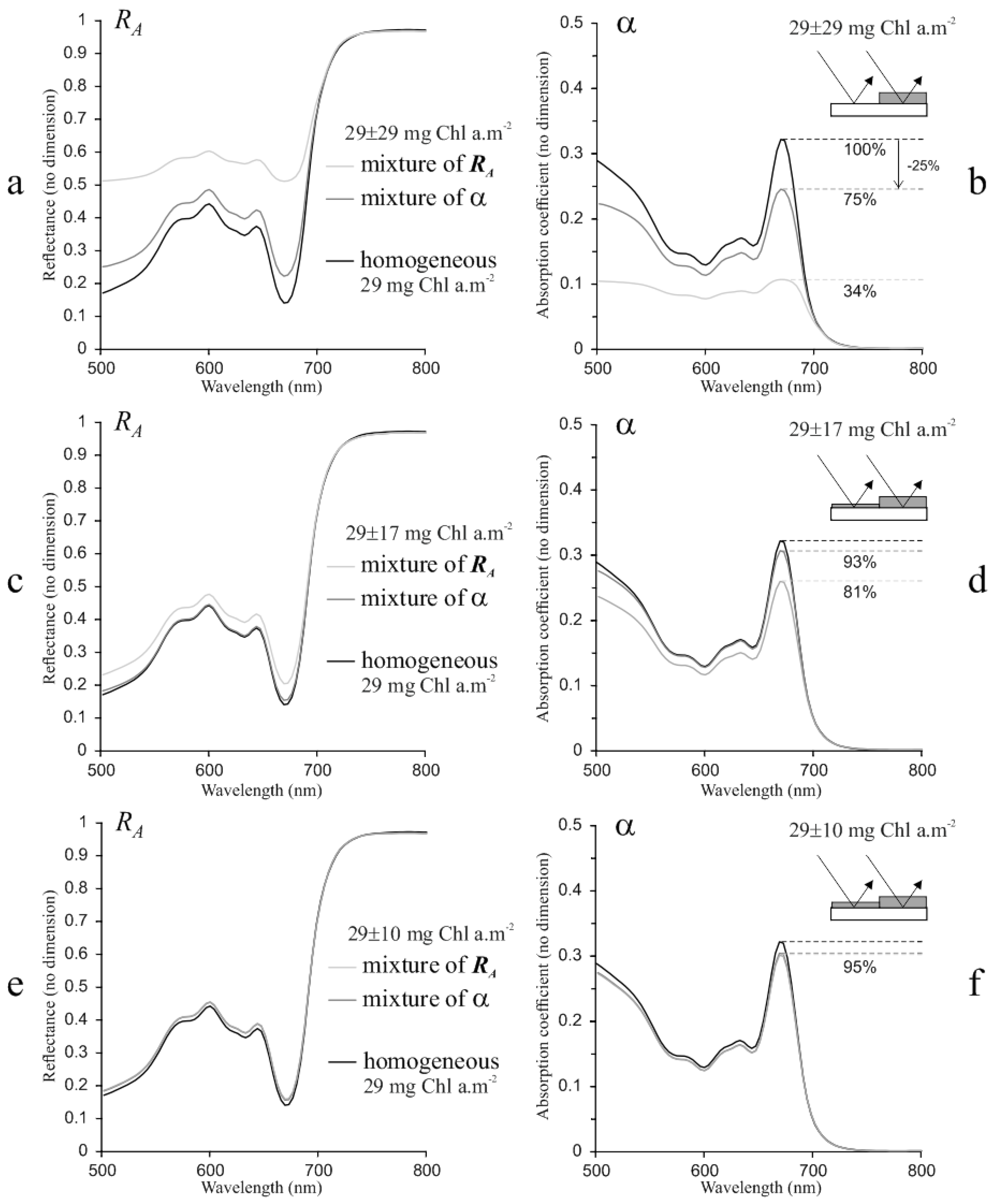
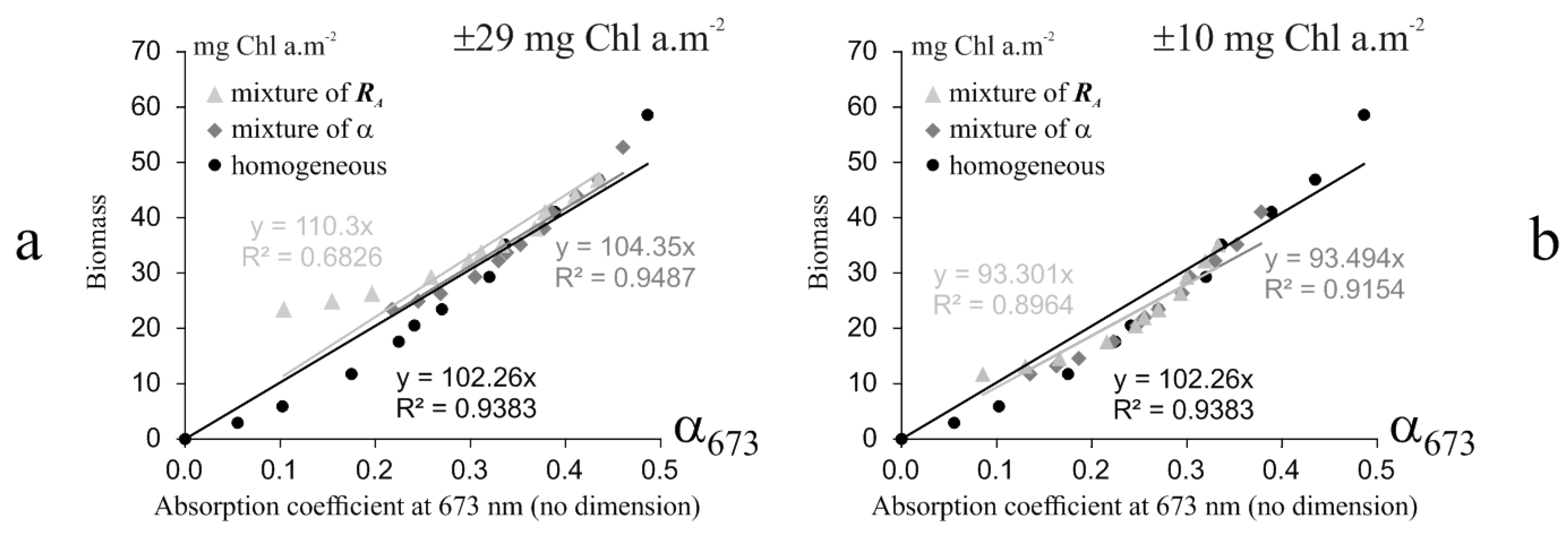
3.1.2. Subpixel Mixing Effects

Mixed pixels were tested (i) by calculating reflectance mixtures following classical studies (e.g., [49]) and (ii) by the calculation of absorption coefficient mixtures with Equation (15) following the MPBOM method.

The R_A mixing of widely scattered MPB biomass ranging from 0 mg Chl a·m⁻² (bare sediment) to 58 mg Chl a·m⁻² (29 ± 29 mg Chl a·m⁻², Figure 8a) and the R_A mixing of moderately scattered MPB biomass ranging from 12 to 47 mg Chl a·m⁻² (29 ± 17 mg Chl a·m⁻², Figure 9c) display spectral differences to the corresponding spectrum with an homogeneous biomass of 29 mg Chl a·m⁻² (Figure 9a,c). When the difference between the two mixed biomass is less pronounced (Figure 9e, mixture of 20 and 41 mg Chl a·m⁻²) spectra showed almost identical patterns to each other. The corresponding α spectrum of strongly and moderately scattered MPB biomass (Figure 9a,b) showed respectively a strong and moderate underestimation of the biomass using the peak of chlorophyll a at 673 nm. Only low scattered and homogeneous MPB biomass can be retrieved with R mixing.

The α mixing of strongly scattered MPB biomass ranging from 0 mg Chl a·m⁻² (bare sediment) to 58 mg Chl a·m⁻² (29 ± 29 mg Chl a·m⁻², Figure 9b) using the sum of subpixel absorption coefficients α prior to apparent reflectance R_A calculation over the background with Equation (15) (mixture of α, Figure 8a,b) display spectra similar to the corresponding α and R_A spectra with homogenous 29 mg Chl a·m⁻² (Figure 9c,b). The chlorophyll a peak at 673 nm of the strongly scattered MPB (29 ± 29 mg Chl a·m⁻², Figure 9b) reaches only 75% of the homogenous MPB chlorophyll a peak at 673 nm but less scattered MPB (29 ± 17 mg Chl a·m⁻², Figure 9d and 29 ± 10 mg Chl a·m⁻², Figure 9f) reach 93% and 95% respectively.

The absorption spectra peak height at 673 nm, remained significantly associated to the biomass in spite of the mixture with R² > 0.91 (Figure 10) while mixing was calculated with α. For instance, unsuitable combinations of R_A gave crushed absorption coefficients and false results in the case of widely scattered biomass (triangles Figure 10a). Only low scattered biomass R_A combinations gave unbiased results (triangles Figure 10b). Thus, α is the only optical parameter which is insensitive to the wide scattering of patchy distribution inherent in MPB biofilms, contrary to R_A which necessitates homogeneity to low scattered MPB within a range of ±10 mg Chl a·m⁻². Therefore, it is recommended to use the linear combination of absorption coefficients to explain subpixel mixtures for which unmixing processes are potentially applicable.

3.2. Images Analyses

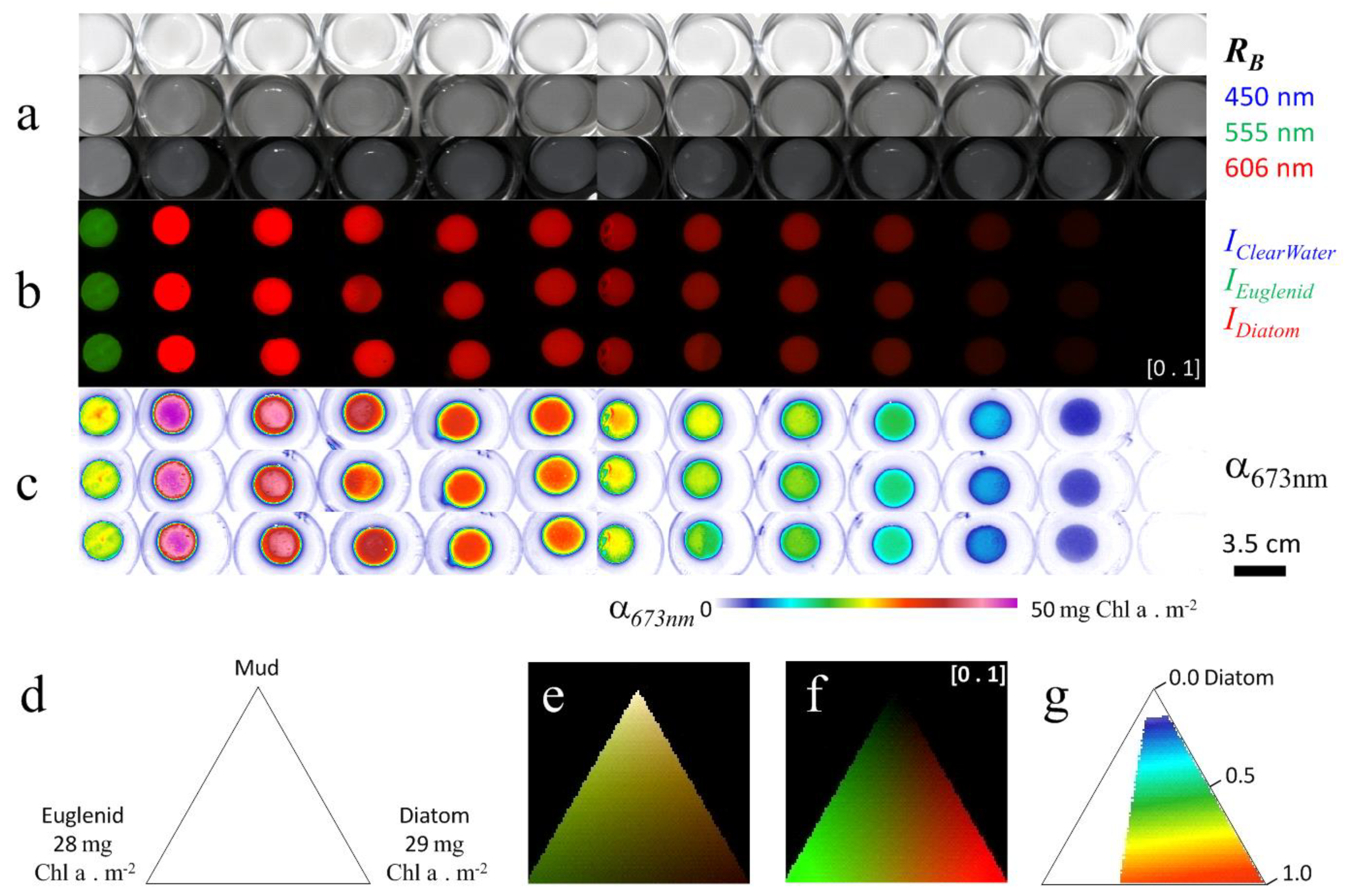
3.2.1. Laboratory Experimentations

Instead of working on 2 cm width ROI of the reflectance image, all calculations were applied at a 0.02 cm pixel size on the full image with monospecific cultures of diatoms and euglenids (Figure 11). All simulated backgrounds R_Bs were similar to each other and all of them showed the absence of absorption bands, showing that the MPBOM can simulate the background whatever the algal composition of the biofilm or biomass (Figure 10a). Three indices were selected to map biofilm composition and water layers: I_ClearWater, I_Diatom and I_Euglenid, displayed with the same standard range [0, 1]. Resulting false colors were proportional to their ranking and allowed an intercomparison at pixel scale without visual bias (Figure 11b). All I_ClearWater pixels were null, without a blue hue, indicating the absence of a water layer (Figure 11b). I_Rhodophyte and I_{Cyanobacteria} were also null (results not shown) whereas the I_Diatom pixels were higher than I_Euglenid for all diatom biofilms displayed in red. Euglenids biofilms were positioned in a single column on the left of the image, and they were characterized by higher I_Euglenid than I_Diatom, appearing as a green color (Figure 11b). The absorption coefficient peak at 673 nm was used to retrieve biomass (Figure 11c) up to 50 mg Chl a·m⁻² using a color code scale.

In preparation for field studies we used the triangular distribution of Figure 11d to simulate in Figure 11e mud pixels covered by two biofilms of euglenid and diatom with comparable biomass (28.4 and 29.3 mg Chl a·m⁻² respectively). Each pixel of the triangle is composed of 100% endmember and the central pixel is composed of 33% euglenid, 33% diatom and 33% uncovered mud. The α mixing was performed with a combination of euglenid and diatom α prior to the calculation of the R_A mixture over the mud R_B with Equation (15) (Figure 11e). As with Figure 11b,f displays [0, 1] the standardized false color of I_ClearWater, I_Diatom and I_Euglenid indices displayed in blue, green and red channel respectively. Uncovered pixels are black, pure euglenid pixels are green and pure diatom are red whereas mixtures between euglenid and diatoms appear orange to brown. The ranking between I_Diatom and I_Euglenid of Table 3 was used to define a mask mapping only chlorophyll a peak of diatom MPB (Figure 11g). The color code of Figure 11c,g are the same but background and pixels dominated by euglenid were removed and appear in white. The biomass range from 5 mg Chl a·m⁻² to 29 mg Chl a·m⁻² for 100% diatom MPB. The NDVI_HR > 0.1 criterion did not allow the detection of the lowest biomass below 5 mg Chl a·m⁻² because of possible confusion with other bare mudflats encountered in the subsequent field studies. The biomass of diatom MPB presented in Figure 11g should always be compared with the 3 indices color composition of Figure 10b where they should appear red for pure diatom MBP or orange for diatom MBP mixed with a low percentage of other MPB types. A brown color may be found between 40% to 50% diatom and 50% to 60% euglenid for which Iα_diatom remains greater than Iα_euglenid. All the settings used in this simulation are identical to those of the following field studies.

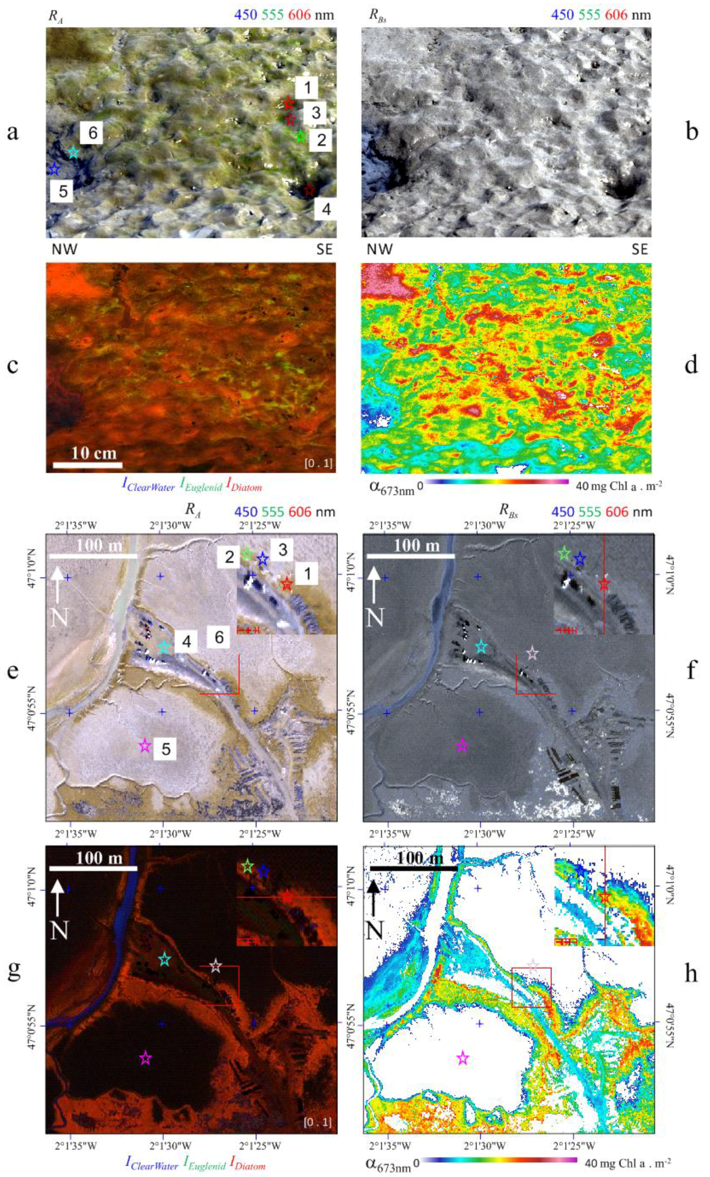
3.2.2. Ground Field Image

Investigation of the ground field image (Figure 12a) was at an intermediate scale between micro-scale at laboratory (Figure 11) and macro-scale with airborne images (Figure 12e). Using the default band selection of true color images provided by the HySpex VNIR camera, diatoms apparent reflectance (R_A) were typically brown whereas euglenids were green (Figure 12a). With the same color composition, simulated background R_Bs were mostly grey with the exception of areas covered by a small amount of water which appeared in blue (Figure 12b). This is due to water absorption at 983 nm (see Figure 4b) inverting the slope of the regression line calculated in the spectral range 750–920 nm to simulate backgrounds (see spectra 5 and 6 Figure 13a). This spectral effect was also detectable with the water index I_ClearWater (Figure 12c). A color composition combining pixels covered with water (blue color), pixels dominated by I_Euglenid or I_Diatom displayed a range of intensity bound to [0, 1] allowed identification of biofilm algal composition: the biofilm was dominated by diatoms (red-orange colors) with smaller patches of green euglenids (Figure 12c). The orange aspect of diatoms (pure diatoms are red, see Figure 11g) could indicate either mixing with low amounts of other MPB or pigment distribution changes due to physiological stress. The diatom biofilm was composed of a network of multi-centimeter patches of various amounts of biomass with a lateral extension apparently driven by the size of the ripple marks. Locally, higher diatom biomass were observed associated to muddy covered ripple marks best seen on the upper left corner of the R_Bs image (Figure 12b). The spatial distribution of diatom biomass is displayed with a color code, ranging from 0.4 to 40 mg Chl a·m⁻², corresponding to the value of the absorption coefficient spectra at 673 nm (Figure 12d). A white mask has been applied to hide pixels colonized by euglenids up to 40% MPB (see also Figure 11g).

Apparent reflectance spectra were collected in 6 ROI (labels and star symbols, Figure 12a) and displayed with their respective absorption spectra (Figure 13a,b). The ROI 5 and 6 displayed strong to moderate absorption features of water at 983 nm. The reflectance spectrum of the ROI 5 (Figure 13a) exhibiting an excessive negative slope of −0.124 R per μm was presented to illustrate the effect of the clear water layer at the top of a MPB (compare with Figure 4b). The ROI 6 reflectance spectrum exhibited a positive slope of the simulated background falling in the range of −0.12 × 10⁻³ to +0.66 × 10⁻³. All other ROI spectra display slope similar to the ROI 6 but displayed a weak absorption band at 983 nm. This confirmed the low impact of interstitial water on the reflectance shape in the VNIR domain (400–900 nm). The ROI 2 spectrum showed the presence of euglenids (Figure 13a). The ROI 1, 3 and 4 spectra were diatom pixels sampled in areas with (ROI 4) and without shadows (ROI 1) created by the ripple marks. The consequence of shadows was a shifting down of the reflectance intensity from ROI 1 to 4 (Figure 13a) which did not alter the calculation of absorption coefficients (Figure 13b).

3.2.3. Airborne Imaging: Mudflat Case Study

The MPBOM was applied at a macroscale of the mudflat. An area of interest (AOI) was selected from airborne images of Bourgneuf bay (Figure 2a), focusing on the site of La Coupelasse (Figure 12e) and a selection of 6 ROI mean spectra (Figure 13). The same camera was used for ground and airborne imaging, but not at the same time: May for the ground field panorama and October for the airborne imagery. The apparent reflectance R_A image displayed brown biofilms (Figure 12e), associated with lighter sediments as revealed by the background reflectance simulation R_Bs (Figure 12f). A strong negative slope of R_Bs (blue pixels in Figure 12f) and indices color compositions allowed the identification of pixels covered with translucent water, including superficial layers at the top of tidal channel (Figure 12g). Biofilms were dominated by diatoms while no euglenids were detected at this scale of observation (Figure 12g) but the orange pixels of the indices color composites revealed a low portion of other MPB as shown in Figure 11 g. The highest biomass was observed at the vicinity of the tidal channels and rocky areas with oyster cultures and wild oyster reefs (Figure 12h).

Six apparent reflectance spectra R_A were collected in 12 pixels (5.7 m²) ROI (star labels in Figure 12e) and displayed with their respective absorption ROI mean spectra (Figure 13b,d). All spectra showed a small absorption band around 950 to 980 nm, confirming the presence of water at the mudflat surface. All displayed moderate negative slopes of their background simulation, between −0.12 and +0.66 μm⁻¹ in reflectance, which did not prevent the use of the model. They were all grey in the R_BS distribution map whereas tidal channels with stronger negative slope appeared blue (Figure 12f). Pixels identified as diatoms in ROI 1 to 3 (Figure 12g and corresponding reflectance spectra in Figure 13c) had a biomass ranging from 7 to 20 mg Chl a·m⁻². The ROI 4 corresponding to a large platform used by oyster farmer vehicles, was covered by mud containing a small amount of diatoms (Figure 12e and Figure 13c,d). The two last ROI 5 and 6 were taken in areas that were not classified as MPB (Figure 12h) because of the NDVI_HR limit of detection set at 0.15 to prevent the misidentification of MPB on large bare mudflats having no MPB as it can be checked in the 3 indices color composition of Figure 12g where all pixels are displayed without any mask. However, a weak absorption band in reflectance and absorption coefficient peak at 673 nm were observed. This suggests that very low biomass cannot be detected because of the masking process as show in Figure 10, or because of the ambiguity between the spectral slope of a neutral sediment and MPB. It is preferable to miss a few pixel of weak MPB biomasses than getting a lot of false positive detection of it.

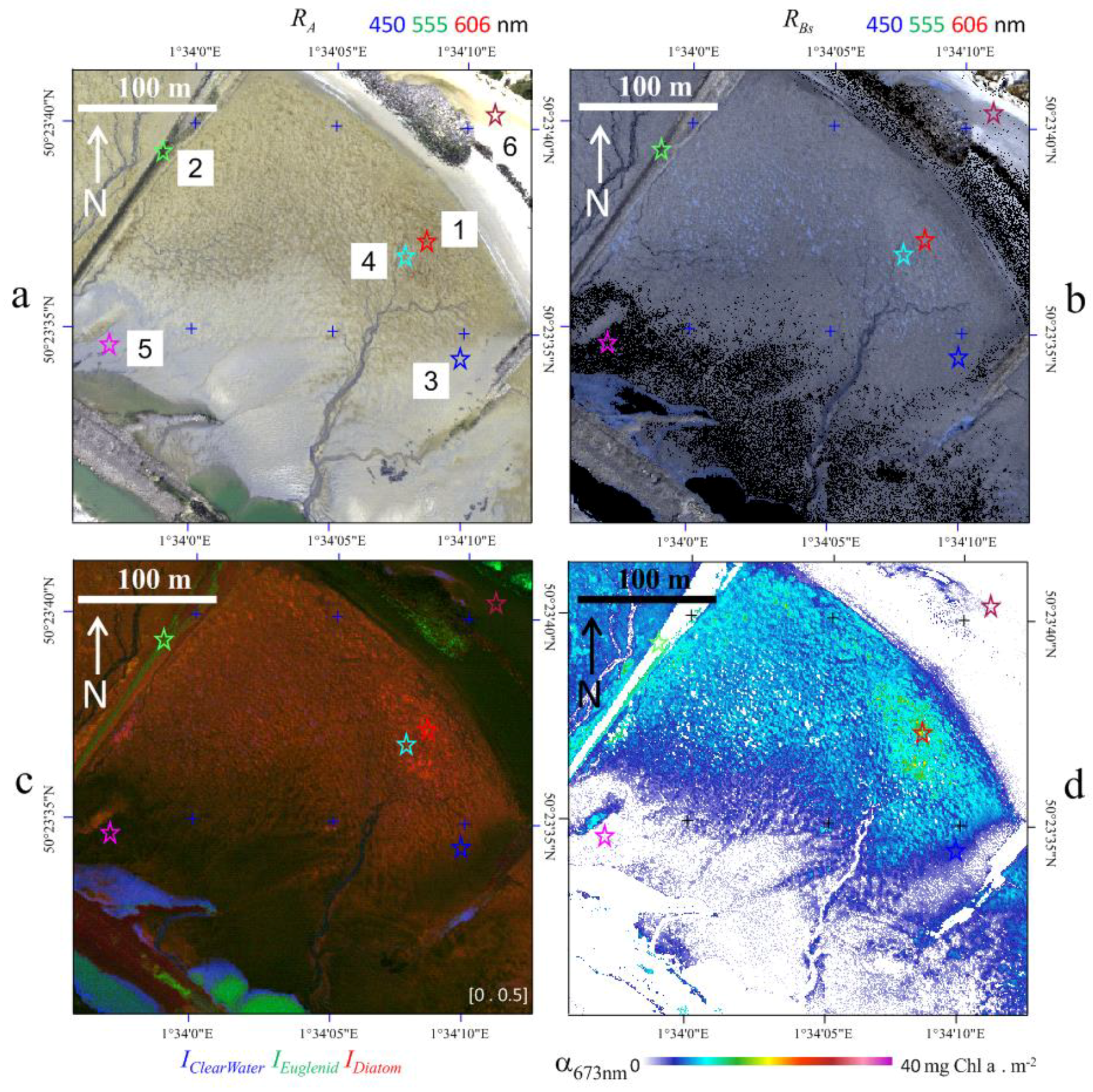
3.2.4. Airborne Imaging: Sandy Case Study

The Authie estuary area of interest (Figure 2b) is mainly characterized by sandy sediment, in sandbanks, in small mudflat areas (Figure 14a). Many pixels were covered by water, and displayed a characteristic strong negative slope of their R_BS. They appeared blue with spherical shapes in the upper intertidal area which corresponded to water puddles (Figure 14b) and then were subsequently masked in the resulting biomass map (Figure 14d). Sandbanks ROI 5 in the south of the AOI image (Figure 14 and spectrum Figure 15a), as with the breakwaters and parts of the beach in the north, displayed simulated backgrounds cutting their own reflectance in the 550–675 nm spectral range as already mentioned in Figure 4. The MPBOM model could not be used for such pixels as their R_BS was set to 0. They appeared in black in Figure 14b and were masked in white in the final biomass map of Figure 14d.

The color composite image displayed a contrasted distribution between diatom biofilms with dominant I_Diatom values and green biofilm with dominant I_Euglenid values (Figure 14c). Sparse macro algae were detected by I_Euglenid index raw display (Figure 14c) but removed by the masking procedure with either I_Euglenid > NDVI_HR or MPBIα > 0 criteria in Figure 14d. The 3 indices color composition help understand the MPB distribution, but it is not a full diagnostic of MPB type which relies on ranking between indices. The biomass distribution map showed that the average and maximum of chlorophyll a concentrations were lower in this sandy estuary compared to the Bourgneuf Bay mudflat (Figure 12h).

The ROI 1 and 4 of Figure 15a,b, were in 12 pixels (5.7 m²) ROI selected for their increasing biomass of diatom biofilm whereas the ROI 2 spectrum displayed a typical green algae reflectance, which grows on breakwaters heavily colonised with barnacles. The ROI 5 corresponds to sandy-silt sediment reflectance with high carbonate content from the shell debris of molluscs and barnacles. Its absorption coefficient was not calculated (Figure 15b) because of the intersection of R_BS with its reflectance between 550 nm and 670 nm. The last sample, ROI 6 spectrum (Figure 15a,b) was taken from the beach not too far from the breakwater and it shows that most sands surfaces displayed a sandy spectrum characterized by a neutral VNIR shape (see also Figure 4).

4. Discussion

4.1. A Simplified Optical Model of MPB Relying on Background

In this work, the optical model of [24,25] was reorganized and completed to estimate MPB biomass for different groups of unicellular photoautotrophs.

First of all, the biomass provided by independent HPLC quantification of the Chl a by measuring its absorption coefficient α after a chromatographic migration allowing its full effective separation from other pigments, we bring back first in the MPBOM method the calculation of the same physical variable α. This absorption coefficient α being linked to the attenuation coefficient η which can be extracted from hyperspectral apparent reflectance R_A, is the most appropriate physical variable of intercalibration between HPLC and hyperspectral data. We simplified the MPBOM model of [24] to its maximum by directly linking α to the ratio between apparent reflectance R_A and background reflectance R_B (Equation (13)). By doing so, we highlighted the importance of the background determination in the MPBOM. When background reflectance R_B is available for example when biofilms are reconstituted on glass-fiber filters deposited on Spectralon^® that can be measured independently [21], R_B can be directly used in the model. In field situations independent measurements of R_B were not available. However, background estimation remains possible by using the calculation of the slope of the regression line in the 750 nm to 920 nm wavelength range as defined by Kazemipour et al. [24] but also used by Chennu et al. [26]. This range corresponds to a 100% transmittance window of MPB biofilms shown by [25] with combination of black and white background. In general, in situ backgrounds for MPB range from muddy to sandy with a positive slope in the VNIR domain [50]. However in Authie Bay, some sediment enriched with barnacle shell debris, displayed such a steep slope, that we introduced a new condition (maximum slope of +0.66 μm⁻¹) to prevent R_Bs straight line estimation to intersect with R_A before 400 nm (i.e., in the visible range). Whereas interstitial water as no impact on background reflectance as shown in Figure 4a, the presence of a thin layer of water at the surface of the mudflat was another constraint for the estimation of R_Bs. A thin clear water let appear the background as shown in Figure 4 b, but it modifies the slope of R_Bs and can bias the calculation of α. A second condition on background estimation (minimum slope of −0.124 μm⁻¹) was added. Waiting a full radiative transfer model of this multi-layered system including a water layer on top of the sediment surface, which will be presented in a forthcoming work, an empirical approach is used to mask non-neutral background and water layers at the surface of the mudflat.

4.2. Identification of the Main MPB Groups

The second improvement to the MPBOM was the discrimination between the different groups of unicellular photoautotrophs composing MPB. MPB biofilms are frequently dominated by diatoms but cyanobacteria, euglenids or chlorophytes may be also present (e.g., [3]). These groups can be identified by the specific association of pigments responsible for characteristic spectral shapes with wells corresponding to absorption features and peaks. We extended the index calculation from R_A to absorption coefficient spectra (α) and replaced the MPB type selection based on multiple arbitrary thresholds by a standalone relative ranking between indices. The only threshold used in this work is applied to the normalized different vegetation index calculated on two channels at high spectral resolution (NDVI_HR). This threshold was used to discard positive NDVI values which can be obtained from bare sediment without MPB, and was set to 0.10 and 0.15 respectively for the sandy and muddy sites. All indices calculated with reflectance (MPBI, I_Diatom, I_Euglinid, I_Rhodophyte, I_{Cyanobacteria}) and based on characteristic spectral wells or peaks were proportional to the biomass (Figure 7b,d) and could be ranked to identify the main groups of MPB (Table 2) covering more than 50% of a pixel. Mixing was however detectable with indices on standardized color composite images. Any departure of each red, green and blue hues of the color composite endmembers indicate a mixing with another MPB group. The absorption coefficient index NDVIα_HR is equal to 1 for all MPB groups and departures from this value of 1 indicate the presence of other types of vegetation with non-null inherent reflectance in the NIR such as macro algae or seagrass fragments. All other α indices (MPBIα, Iα_Diatom, Iα_Euglinid, Iα_Rhodophyte, and Iα_{Cyanobacteria}) were uncorrelated with biomass (Figure 7f,h) and could be ranked to identify the main groups of MPB (Table 3). The advantage of working with α spectra is that shape analysis to identify the main MPB groups and biomass estimation can be done separately. The α values provided from reflectance by the MPBOM can be directly correlated with independent absorption measurements provided by HPLC chromatograms calibrated in the biomass.

All variations of pigment distributions, often linked to physiological variations, can now be studied with the help of α indices independently of the biomass. Moreover, the independence of the α spectral shapes to the biomass, at least in the (650–700 nm) Chl a absorption band, means that any biomass spectrum can be obtained by a simple weighing of the spectrum of a specific α endmember. Therefore, any α spectral biomass can be calculated with a linear combination of α endmember and conversely α unmixing procedures are applicable. However, unmixing is extremely sensitive to pigment variations and the influence of short-term physiological changes will be explored in another study.

4.3. Sub-Pixel Mixing

The subpixel analysis supposes that each heterogeneous pixel can be obtained by the aggregation of smaller subpixels. This is the basic principle of all unmixing [49] and this was used also by [23] to map MPB with a Digital Airborne Imaging Spectrometer (DAIS) hyperspectral sensor from GER (Geophysical Environmental Research Corporation) of Milbrook, N.Y., USA. This work, preliminary to any unmixing study, aim to identify which variable are compatible with linear combinations of endmembers. So we combined the apparent reflectance of two endmembers of MPB with background with a set of 12 different biomasses to show that their combinations cannot reproduce the reflectance of a homogeneous biofilm, unless the difference between the two endmembers is smaller than 10 mg Chl a·m⁻². Higher heterogeneities required a separation between background and MPB biofilm which must be processed separately and eventually recombined for scale change calculations. Opaque backgrounds can be combined in reflectance as simple mixing whereas translucent MPB biofilm must be combined as intimate mixing in absorption coefficients. With such protocol the influence of subpixel mixing was strongly reduced. The underestimation range from −2% to −5% but a maximum of −25% (see Figure 8b) was found with the most contrasted combinations. This study explored subpixel mixing effects at microscale by their aggregation in pixel with the analysis of optical properties of monospecific cultures of diatoms and euglenids synthetized in the laboratory. At a metric scale, euglenids could be observed in the field as small but distinct patches mixed within larger diatom biofilms. However, at the coarser spatial resolution of airborne images, euglenids were no longer visible, only diatoms, but some pixels were likely to be composed of a mixing between euglenids and diatoms. This subpixel contains are clearly detected by the indices of the color composite images that were produced in addition to the biomass maps. But this comparison and ranking between indices only determine the main MPB type. The identification of the small amount of another MBP type in a pixel dominated by one MPB type would require α unmixing procedure which will be done in a future work as already discussed in Section 4.2.

Successive spatial measurements corresponded to pixel sizes of 0.0002 m in the laboratory, to 0.002 m in panoramic views and 0.7 m in airborne images. The ground image presented in Figure 11 corresponds to approximately one airborne pixel. It clearly shows a network of more or less homogenous MPB patches of a few centimeters wide which confirm the observation of [23,26,32]. The full calibration of the area of an airborne 0.7 × 0.7 m pixel would require the sampling of 0.49 m² of MPB on the ground which is in practice not feasible. MPB sediment sampling with contact-cores, plastic tubes or syringes are never performed at this spatial scale [30] without the help of kriging method [32]. Sampling by in situ freezing often relies on 20 cm² cores [51,52]. The full calibration of the 0.7 × 0.7 m single-pixel coverage with 20 cm² contact-cores would require 245 samples which is unrealistic. This difficulty of perfect matching between field samples and pixels was bypassed with the MPBOM allowing the extraction of the absorption coefficient of a given biomass of a MPB biofilm, independent of its background. The validation of the method is done with monospecific cultures in the laboratory at microscale with a Hyspex camera and concomitant HPLC measurements of chlorophyll a based on absorption coefficient giving slope of best regression line with comparable hyperspectral absorption coefficient peak at 673 nm. For the airborne images, only spectroradiometric data were collected on a set of ground control points to ensure the perfect match between airborne and ground neutral references.

5. Conclusions

The MPBOM [24,25] was shortened to a straightforward calculation of α (Equation (13)) from the ratio between an apparent reflectance and a background reflectance with the MPB as negligible inherent reflectance. We showed in this study that all backgrounds are not suitable for MPBOM calculations and outlined new limitations to the MPBOM application as for example in the case of thin water layers at the top of the MPB or sand enriched barnacle debris containing organic absorption features altering the separation between MPB and mineral background.

In order to promote the use of the absorption coefficient we developed and validated a new equation (Equation (15)) to calculate the apparent reflectance of a MPB mixture R_A over a background R_B with a combination of individual MPB absorption coefficient α. This equation was developed to separate the background reflectance R_B from its multiplication by a linear combination of mixed MPB α biofilm. To summarize, the MPBOM suggests that backgrounds are opaque additive reflectance spectra time combinations of translucent multiplicative absorption coefficients of biofilms. Therefore, any change in scale would require a decomposition of all MPB spectra in opaque backgrounds and translucent biofilm components to be processed separately as also summarized in the new workflow presented in Figure 16.

This work confirms that indices based on reflectance measuring the height of well and peak characteristics of pigment association correctly identified the main MPB groups covering a pixel. By developing the use of α and the setting of new indices based on absorption coefficients, this work showed that pigment association characteristics of MPB groups were independent of the biomass, opening up a new field of studies where the proportion between pigments can be monitored independently of the total amount of biomass. Conversely it has been established that the height of α peak is proportional to the biomass which implies that weighing it can simulate any intermediate biomass when it is separated from its background. The next challenge is now to correctly unmix the pigment absorption coefficients including degradation pigments in order to clearly define endmembers.

References

1. Kazemipour, F.; Méléder, V.; Launeau, P. Optical properties of microphytobenthic biofilms (MPBOM): Biomass retrieval implication. J. Quant. Spectrosc. Radiat. Transf. 2011, 112, 131–142. [Google Scholar] [CrossRef]
2. Kazemipour, F.; Launeau, P.; Méléder, V. Microphytobenthos biomass mapping using the optical model of diatom biofilms: Application to hyperspectral images of Bourgneuf Bay. Remote Sens. Environ. 2012, 127, 1–13. [Google Scholar] [CrossRef]
3. Underwood, G.J.C.; Smith, D.J. Predicting Epipelic Diatom Exopolymer Concentration in Intertidal Sediments from Sediment Chlorophyll a. Microb. Ecol. 1998, 35, 116–125. [Google Scholar] [CrossRef] [PubMed]
4. Heip, C.H.R; Goosen, N.K.; Herman, P.M.J.; Kromkamp, J.; Middelburg, J.J.; Soetaert, K. Production and consumption of biological particles in temperate tidal estuaries. Oceanogr. Mar. Biol. Annu. Rev. 1995, 33, 1–149. [Google Scholar]
5. MacIntyre, H.; Geider, R.; Miller, D. Microphytobenthos: The ecological role of the “secret garden” of unvegetated, shallow water marine habitats. I. Distribution, abundance and primary production. Estuaries 1996, 19, 186–201. [Google Scholar] [CrossRef]
6. Hoppenrath, M.; Murray, S.A.; Chomerat, N.; Horiguchi, T. Marine Benthic Dinoflagellates: Unveiling Their Worldwide Biodiversity; Schweizerbart Science Publishers: Stuttgart, Germany, 2014; 276p. [Google Scholar]
7. Barillé, L.; Le Bris, A.; Méléder, V.; Launeau, P.; Robin, M.; Louvrou, I.; Ribeiro, L. Photosynthetic epibionts and endobionts of pacific oyster shells from oyster reefs in rocky versus mudflat shores. PLoS ONE 2017, 12, e0185187. [Google Scholar] [CrossRef] [PubMed]
8. Jeffrey, S.W. Application of pigment method to oceanography. In Phytoplankton Pigments in Oceanography. Monographs on Oceanographic Methodology; Jeffrey, S.W., Mantoura, R.F.C., Wright, S.W., Eds.; UNESCO Publishing: Paris, France, 1997; pp. 127–166. [Google Scholar]
9. Consalvey, M.; Jesus, B.; Perkins, R.G.; Brotas, V.; Underwood, G.J.C.; Paterson, D.M. Monitoring migration and measuring biomass in benthic biofilms: The effects of dark/far-red adaptation and vertical migration on fluorescence measurements. Photosynth. Res. 2004, 81, 91–101. [Google Scholar] [CrossRef] [PubMed]
10. Pinckney, J.; Zingmark, R.G. Biomass and Production of Benthic Microalgal Communities in Estuarine Habitats. Estuaries 1993, 16, 887–897. [Google Scholar] [CrossRef]
11. Paterson, D.M.; Black, K.S. Water flow, sediment dynamics and benthic biology. Adv. Ecol. Res. 1999, 29, 155–193. [Google Scholar]
12. De Jonge, V.N.; Van Beuselom, J.E.E. Contribution of resuspended microphytobenthos to total phytoplankton in the EMS estuary and its possible role for grazers. Neth. J. Sea Res. 1992, 30, 91–105. [Google Scholar] [CrossRef]
13. Hernández Fariñas, T.; Ribeiro, L.; Soudant, D.; Belin, C.; Lampert, L.; Bacher, C.; Barillé, L. Contribution of benthic microalgae to the temporal variation in phytoplanktonic assemblages in a macrotidal system. J. Phycol. 2017, 5, 1020–1034. [Google Scholar] [CrossRef] [PubMed]
14. Decottignies, P.; Beninger, P.G.; Rincé, Y.; Riera, P. Trophic interactions between two introduced suspension-feeders, Crepidula fornicata and Crassostrea gigas, are influenced by seasonal effects and qualitative selection capacity. J. Exp. Mar. Biol. Ecol. 2007, 42, 231–241. [Google Scholar] [CrossRef]
15. Riera, P. Trophic plasticity of the gastropod Hydrobia ulvae within an intertidal bay (Roscoff, France): A stable isotope evidence. J. Sea Res. 2010, 63, 78–83. [Google Scholar] [CrossRef]
16. Cartaxana, P.; Jesus, B.; Brotas, V. Pheophorbide and pheophytin a-like pigments as useful markers for intertidal microphytobenthos grazing by Hydrobia ulvae. Estuar. Coast. Shelf Sci. 2003, 58, 293–297. [Google Scholar] [CrossRef]
17. Kuwae, T.; Beninger, P.G.; Decottignies, P.; Mathot, K.J.; Loud, D.; Elner, R.W. Biofilm grazing in a higher vertebrate: The Western Sandpiper Caliders mauri. Ecology 2008, 89, 599–606. [Google Scholar] [CrossRef] [PubMed]
18. Forster, R.M.; Kromkamp, J.C. Estimating benthic primary production: Scaling up from point measurements to the whole estuary2006. In Functioning of Microphytobenthos in Estuaries; Kromkamp, J.C., de Brouwer, J.F.C., Blanchard, G.F., Forster, R.M., Creach, V., Eds.; Royal Netherlands Academy of Arts and Sciences: Amsterdam, the Netherlands, 2006; pp. 109–120. [Google Scholar]
19. Ubertini, M.; Lefebvre, S.; Gangnery, A.; Grangeré, K.; Gendre, R.L.; Orvain, F. Spatial variability of benthic-pelagic coupling in an estuary ecosystem: Consequences for microphytobenthos resuspension phenomenon. PLoS ONE 2012, 7, e44155. [Google Scholar] [CrossRef] [PubMed]
20. Tucker, C.J. Red and photographic infrared linear combinations for monitoring vegetation. Remote Sens. Environ. 1979, 8, 127–150. [Google Scholar] [CrossRef]
21. Benyoucef, I.; Blandin, E.; Lerouxel, A.; Jesus, B.; Rosa, P.; Meleder, V.; Launeau, P.; Barillé, L. Microphytobenthos interannual variations in a north-European estuary (Loire estuary, France) detected by visible-infrared multispectral remote sensing. Estuar. Coast. Shelf Sci. 2014, 136, 43–52. [Google Scholar] [CrossRef]
22. Brito, A.C.; Benyoucef, I.; Jesus, B.; Brotas, V.; Gernez, P.; Mendes, C.R.; Launeau, P.; Dias, P.; Barillé, L. Seasonality of microphytobenthos revealed by remote-sensing in a South European estuary. Cont. Shelf Res. 2013, 66, 83–91. [Google Scholar] [CrossRef]
23. Méléder, V.; Barillé, L.; Launeau, P.; Carrère, V.; Rincé, Y. Spectrometric constraint in analysis of benthic diatom biomass using monospecific cultures. Remote Sens. Environ. 2003, 88, 386–400. [Google Scholar] [CrossRef]
24. Van der Wal, D.; Wielemaker-van den Dool, A.; Herman, P.M. Spatial synchrony in intertidal benthic algal biomass in temperate coastal and estuarine ecosystems. Ecosystems 2010, 13, 338–351. [Google Scholar] [CrossRef]
25. Combe, J.P.; Launeau, P.; Carrere, V.; Despan, D.; Meleder, V.; Barillé, L.; Sotin, C. Mapping microphytobenthos biomass by non-linear inversion of visible-infrared hyperspectral images. Remote Sens. Environ. 2005, 98, 371–387. [Google Scholar] [CrossRef]
26. Jesus, B.; Rosa, P.; Mouget, J.-L.; Meleder, V.; Launeau, P.; Barillé, L. Spectral-radiometric analysis of taxonomically mixed microphytobenthic biofilms. Remote Sens. Environ. 2014, 140, 196–205. [Google Scholar] [CrossRef]
27. Chennu, A.; Färber, P.; Volkenborn, P.; Al-Najjar, M.A.A.; Janssen, F.; de Beer, D.; Polerecky, L. Hyperspectral imaging of the microscale distribution and dynamics of microphytobenthos in intertidal sediments. Limnol. Oceanogr. Methods 2013, 11, 511–528. [Google Scholar] [CrossRef] [Green Version]
28. Nogami, S.; Ohnuki, S.; Ohya, Y. Hyperspectral imaging techniques for the characterization of haematococcus pluvialis (chlorophyceae). J. Phycol. 2014, 50, 939–947. [Google Scholar] [CrossRef] [PubMed]
29. Méléder, V.; Laviale, M.; Jesus, B.; Mouget, J.-L.; Lavaud, J.; Kazemipour, F.; Launeau, P.; Barillé, L. In vivo estimation of pigment composition and optical absorption cross-section by spectroradiometry in four aquatic photosynthetic micro-organisms. J. Photochem. Photobiol. B 2013, 129, 115–124. [Google Scholar] [CrossRef] [PubMed] [Green Version]
30. Méléder, V.; Launeau, P.; Barillé, L.; Combe, J.P.; Carrère, V.; Jesus, B.; Verpoorter, C. Hyperspectral imaging for mapping microphytobenthos in coastal areas. In Geomatic Solutions for Coastal Environments; Maanan, M., Robin, M., Eds.; Nova Science Publishers, Inc.: Hauppauge, NY, USA, 2010; pp. 71–139. [Google Scholar]
31. Saburova, M.A.; Polikarpov, I.G.; Burkovsky, I.V. Spatial structure of an intertidal sandflat microphytobenthic community as related to different spatial scales. Mar. Ecol. Prog. Ser. 1995, 129, 229–239. [Google Scholar] [CrossRef]
32. Spilmont, N.; Seuront, L.; Meziane, T.; Welsh, D.T. There’s more to the picture than meets the eye: Sampling microphytobenthos in a heterogeneous environment. Estuar. Coast. Shelf Sci. 2011, 95, 470–476. [Google Scholar] [CrossRef]
33. Richter, R.; Schläpfer, D. Atmospheric /Topographic Correction for Airborne Imagery; DLR Report DLR-IB 565-02/14, 240; DLR: Wessling, Germany, 2014. [Google Scholar]
34. Green, A.A.; Berman, M.; Switzer, P.; Craig, M.D. A Transformation for Ordering Multispectral Data in Terms of Images Quality with Implications for Noise Removal. IEEE Trans. Geosci. Remote Sens. 1988, 26, 65–74. [Google Scholar] [CrossRef]
35. Boardman, J.W.; Kruse, F.A. Automated Spectral Analysis: A Geologic Example using AVIRIS Data, North Grapevine Mountains, Nevada. In Proceedings, ERIM Tenth Thematic Conference on Geologic Remote Sensing; Environmental Research Institute of Michigan: Ann Arbor, MI, USA, 1994; pp. I-407–I-418. [Google Scholar]
36. Decottignies, P.; Beninger, P.G.; Rincé, Y.; Robbins, R.J.; Riera, P. Exploitation of natural food sources by two sympatric, invasive suspension-feeders: Crassostrea gigas and Crepidula fornicata. Mar. Ecol. Prog. Ser. 2007, 334, 179–192. [Google Scholar] [CrossRef]
37. Dobroniak, C.; Anthony, E.J. Short-term morphological expression of dune sand recycling on a macrotidal, wave-exposed estuarine shoreline. J. Coast. Res. 2002, 36, 240–248. [Google Scholar] [CrossRef]
38. Marion, C.; Anthony, E.J.; Trentesaux, A. Short-term estuarine mudflat and salt-marsh sedimentation: High-resolution data from ultrasonic altimetry, rod surface-elevation table, and filter traps. Estuar. Coast. Shelf Sci. 2009, 83, 475–484. [Google Scholar] [CrossRef]
39. Pye, K.; French, P. Erosion and Accretion Processes on British salt Marshes. In Introduction: Saltmarsh Processes and Morphology; Cambridge Environmental Research Consultants: Cambridge, UK, 1993; Volume 1. [Google Scholar]
40. Deloffre, J.; Verney, R.; Lafite, R.; Lesueur, P.; Lesourd, S.; Cundy, A.B. Sedimentation on intertifal mudflats in the lower part of macrotifal estuaries: Sedimentation rythms and their preservation. Mar. Geol. 2007, 241, 19–32. [Google Scholar] [CrossRef]
41. Carrère, V.; Spilmont, N.; Davoult, D. Comparison of simple techniques for estimating chlorophyll a concentration in the intertidal zone using high spectral-resolution field-spectrometer data. Mar. Ecol. Prog. Ser. 2004, 274, 31–40. [Google Scholar] [CrossRef]
42. Jacquemoud, S.; Baret, F. PROSPECT: A model of leaf optical properties spectra. Remote Sens. Environ. 1990, 34, 75–91. [Google Scholar] [CrossRef]
43. Khashan, M.; El-Naggar, A. A new method of finding the optical constants of a solid from the reflectance and transmittance spectrograms of its slab. Opt. Commun. 2000, 174, 445–453. [Google Scholar] [CrossRef]
44. Astachov, L.; Nevo, Z.; Brosh, T.; Vago, R. The structural, compositional and mechanical features of the calcite shell of the barnacle Tetraclita rufotincta. J. Struct. Biol. 2011, 175, 311–318. [Google Scholar] [CrossRef] [PubMed]
45. Johnsen, G.; Sakshaug, E. Biooptical characteristics of PSII and PSI in 33 species (13 pigment groups) of marine phytoplankton, and the relevance for pulse-amplitude-modulated and fast-repetition-rate fluorometry1. J. Phycol. 2007, 43, 1236–1251. [Google Scholar] [CrossRef]
46. Kazemipour, F. Caractérisation Hyperspectrale des Biofilms Microphytobentiques: Cartographie de la Biomasse de la Micro à la Macro Échelle. Ph.D. Thesis, Université de Nantes, Nantes, France, 2011; p. 204. [Google Scholar]
47. Launeau, P.; Girardeau, J.; Sotin, C.; Tubia, J. Comparison between field measurements and airborne visible and infrared mapping spectrometry (AVIRIS and HyMap) of the Ronda peridotite massif (south-west Spain). Int. J. Remote Sens. 2004, 25, 2773–2792. [Google Scholar] [CrossRef]
48. Carrère, V.; Conel, J.E. Recovery of atmospheric water vapor total column abundance from imaging spectrometer data around 940 nm-sensitivity analysis and application to Airborne Visible/Infrared Imaging Spectrometer (AVIRIS) data. Remote Sens. Environ. 1993, 44, 179–204. [Google Scholar] [CrossRef]
49. Roberts, D.A.; Gardner, M.; Church, R.; Ustin, S.; Scheer, G.; Green, R.O. Mapping chaparral in the Santa Monica Mountains using multiple endmember spectral mixture models. Remote Sens. Environ. 1998, 65, 267–279. [Google Scholar] [CrossRef]
50. Barillé, L.; Mouget, J.-L.; Méléder, V.; Rosa, P.; Jesus, B. Spectral response of benthic diatoms with different sediment backgrounds. Remote Sens. Environ. 2011, 115, 1034–1042. [Google Scholar] [CrossRef]
51. Paterson, D.M.; Wiltshire, K.H.; Miles, A.; Blackburn, J.; Davison, I.; Yates, M.G.; McGrorty, S.; Eastwood, J.A. Microbiological mediation of spectral reflectance from intertidal cohesive sediments. Limnol. Oceanogr. Methods 1998, 43, 1207–1221. [Google Scholar] [CrossRef]
52. Grinham, A.R.; Carruthers, T.J.B.; Fisher, P.L.; Udy, J.W.; Dennison, W.C. Accurately measuring the abundance of benthic microalgae in spatially variable habitats. Limnol. Oceanogr. Methods 2007, 5, 119–125. [Google Scholar] [CrossRef]
Figure 1. Hyperspectral mosaic image of apparent reflectance (RA) of euglenid (Euglena gracilis) and diatom (Entomoneis paludosa) from laboratory cultures with different biomass on three backgrounds (RB) of increasing reflectance (20 to 99%). Red green blue (RGB) colors associated with channels at 606, 555 and 450 nm, respectively).
Remotesensing 10 00716 g001
Figure 2. Field study locations (see map of France) of airborne images of (a) 17 October 2016 Bourgneuf bay south of the town of La Bernerie showing large MPB areas on mudflats more or less abundant in oyster farms (grey arrows) and wild oyster (white arrow) and (b) 21 September 2016 Authie estuary south of the town Berck-Plage showing narrow MPB areas on sandflats; (c) ground field panorama of La Coupelasse mudflat imaged with a camera set up on a rotating stage and view angles ranging from 36° to 54°. RGB color compositions used channels at 606, 555 and 450 nm respectively and red boxes are areas of interest (AOI) detailed in Section 3.
Remotesensing 10 00716 g002
Figure 3. Theoretical diagram of a MPB biofilm formed at the surface of a mudflat. Black arrows are light path reflected once on the background (RB) and transmitted twice through the cells (RA). Diatom cells can be scattered (cell on background in xi next to uncovered background in xj), side by side or stacked on the top of each other (in xk) to form various thicknesses (h) assimilated to various biomass (estimated by the attenuation coefficient α).
Remotesensing 10 00716 g003
Figure 4. Collections of (a) in situ background apparent reflectance RA and their background simulation (straight lines) RBs. For dry sandy sediments from the top of beaches like for other wet sediments of mudflats, lines do not intersect with reflectance spectra. A spectrum of a sandbank with shell debris and a barnacle shells show RBs intersecting reflectance spectra, a condition for which the MPBOM model cannot be applied. This is also the case when mud is covered by a water layer creating a negative slope of RBs due to water absorption features; panel (b) is a collection of clear water on a 99% Spectralon® showing a strong absorption feature starting at 950 nm with a maximum at 983 nm with bands selection of the water detection in VNIR images.
Remotesensing 10 00716 g004
Figure 5. Correlation between absorption coefficient peaks at 673 nm and biomass measured by High Performance Liquid Chromatography (HPLC) in mg Chl a·m−2: (a) row data from Kazemipour et al. [25] and Kazemipour [46] (the grey area is the domain of application of the mudflat); (b) same data set plotted in log-log diagram showing the MPBOM ability to analyze any biomass level but without status health effect.
Remotesensing 10 00716 g005
Figure 6. Spectral library of diatom (Cylindrotheca sp), chlorophyte (Dunaliella sp), cyanobacteria (Spirulina sp) and rhodophyte (Porphyridium sp) from [28] in (a) reflectance R and (b) absorption coefficient α. Curvature of the spectral arc of (c) reflectance and (d) absorption coefficients and bands used to calculate indices with 3 bands presented in Table 1. Grey lines are borders and the black line is the center of the MPBI index in which narrower spectral ranges are used for IDiatom, IEuglenid, ICyanobacteria and IRhodophyte allow the identification of MBP groups. The same index IEuglenid is used both for euglenids and chlorophytes.
Remotesensing 10 00716 g006
Figure 7. Apparent reflectance spectra, RA (a,c) of diatom biofilms of varied biomass on two backgrounds RB (99% and 20%) and their corresponding indices (b,d) from laboratory images. Absorption coefficient spectra, α (e,g) of diatom biofilms of varied biomass on two backgrounds (99% and 20%) and their corresponding indices (f,h) retrieved from laboratory images. Reflectance, absorption coefficient and index intensity are dimensionless parameters contrary to the biomass which is given in mg of Chlorophyll a per m2.
Remotesensing 10 00716 g007
Figure 8. Linear regression between biomass and absorption coefficients at 673 nm with (a) white (99%) and (b) black (20%) background; (c,d) application to other MPB group of [25] library.
Remotesensing 10 00716 g008
Figure 9. Comparison between various mixings of apparent reflectance RA and absorption coefficient α for one mean biomass (RA29): RA of one homogenous biofilm(black line), RA of α mixing (dark grey line), RA mixing (light grey line) of (a) 0 and 58 mg Chl a·m−2; (c) 12 and 47 mg Chl a·m−2 and (e) 20 and 41 mg Chl a·m-2 biomass; α of one homogenous biofilm (black line), α mixing (dark grey line), α of RA mixing (light grey line) of (b) 0 and 58 mg Chl a·m−2; (d) 12 and 47 mg Chl a·m−2 and (f) 20 and 41 mg Chl a·m−2 biomass; broken lines are relative height of α peak at 673 nm equivalent to relative abundance to the mean biomass of 29 mg Chl a·m−2 .
Remotesensing 10 00716 g009
Figure 10. Correlation between absorption coefficients given by all methods plotted with dots for α of homogenous biofilm, diamonds for α mixing and triangles for α of RA mixing of (a) 0 and 58 mg Chl a·m−2 and (b) 12 and 47 mg Chl a·m−2 biomass.
Remotesensing 10 00716 g010
Figure 11. Application of the MPBOM optical model to the mosaic image presented in Figure 1: (a) background simulation, RBS; (b) color composition of 3 indices; (c) α peak at 673 nm with a color code of the corresponding biomass. Microscale heterogeneity of the biofilm due to the filtration of cells on filter supports is visible. Higher biomass were always in the center of the filters and decreased toward the border. The simulation of mixing of (d) 3 endmembers produces in (e) a synthetic image from which (f) displays the color composition of the indices presented in (b) showing euglenids in green, diatoms in red and intermediate MPB in orange to brown; (g) MPBOM results of chlorophyll a peak for α mixing with diatom selection mask and color code of (c).
Remotesensing 10 00716 g011
Figure 12. Area of interest (see Figure 3c) panoramic view of La Coupelasse: (a) apparent reflectance; (b) background simulation highligthing water negative slope in blue; (c) color composition of 3 indices displayed with the same range of intensity [0, 1] and (d) map of absorption coefficient peak at 673 nm with a color code in mg Chl a·m−2. The same color code was applied to Figure h. A peak of 0.4 gives 40 mg Chl a·m−2. Area of interest, La Coupelasse, in the airborne mosaic of Bourgneuf bay (Figure 3b); (e) apparent reflectance, RA; (f) background simulation highligthing water negative slope in blue, RBs; (g) color composition of three indices displayed with the same range of intensity {0, 1} and (h) map of absorption coefficient peak at 673 nm with a color code in mg Chl a·m−2. The upper corner of each image is a close up of the red square centered on the ground study site. Star symbols are the location of reflectance and absorption coefficient of 12 pixels ROI mean spectra shown Figure 12.
Remotesensing 10 00716 g012
Figure 13. Selection of 12 pixels (~12 mm2) ROI mean spectra corresponding to the star symbols in Figure 11a and plotted with the same color code: (a) apparent reflectance RA and corresponding simulated background RBS for Figure 11a; (b) absorption coefficients α. Selection of 12 pixels (5.7 m2) ROI in Figure 11e; (c) apparent reflectance RA and corresponding simulated background RBS; (d) absorption coefficients α.
Remotesensing 10 00716 g013
Figure 14. Area of interest of the airborne Authie mosaic (see Figure 3a); (a) apparent reflectance, RA, with 6 ROI labels; (b) background simulation highlighting water negative slope in blue, RBs; (c) color composition of 3 indices displayed with the same range of intensity [0, 0.5] and (d) map of absorption coefficient peak at 673 nm with a color code in mg Chl a·m−2. A peak of 0.4 gives 40 mg Chl a·m−2. Star symbols are the locations of reflectance and absorption coefficient of 12 pixels ROI mean spectra shown in Figure 13.
Remotesensing 10 00716 g014
Figure 15. Selection of 12 pixels (5.7 m2) ROI mean spectra plotted with the color code of their location label in Figure 13: (a) are reflectances and (b) are their corresponding absorption coefficients.
Remotesensing 10 00716 g015
Figure 16. Final workflow of the MPBOM application showing the link between experimentation in laboratory and calibration of ground and airborne field studies. Large arrows mark the main data entrances and thin arrows are workflow links between MPBOM calculation steps.
Remotesensing 10 00716 g016