Article

A Descriptor-less Well-Distributed Feature Matching Method Using Geometrical Constraints and Template Matching

by
Hani Mahmoud Mohammed
* and
Naser El-Sheimy
Department of Geomatics Engineering, University of Calgary, 2500 University Dr. N.W. Calgary, AB T2N 1N4, Canada
*
Author to whom correspondence should be addressed.
Remote Sens. 2018, 10(5), 747; https://doi.org/10.3390/rs10050747
Submission received: 8 April 2018 / Revised: 7 May 2018 / Accepted: 7 May 2018 / Published: 11 May 2018
(This article belongs to the Section Remote Sensing Image Processing)

Abstract

:
The problem of feature matching comprises detection, description, and the preliminary matching of features. Commonly, these steps are followed by Random Sample Consensus (RANSAC) or one of its variants in order to filter the matches and find a correct model, which is usually the fundamental matrix. Unfortunately, this scheme may encounter some problems, such as mismatches of some of the features, which can be rejected later by RANSAC. Hence, important features might be discarded permanently. Another issue facing the matching scheme, especially in three-dimensional (3D) reconstruction, is the degeneracy of the fundamental matrix. In such a case, RANSAC tends to select matches that are concentrated over a particular area of the images and rejects other correct matches. This leads to a fundamental matrix that differs from the correct one, which can be obtained using the camera parameters. In this paper, these problems are tackled by providing a descriptor-less method for matching features. The proposed method utilises the geometric as well as the radiometric properties of the image pair. Starting with an initial set of roughly matched features, we can compute the homography and the fundamental matrix. These two entities are then used to find other corresponding features. Then, template matching is used to enhance the predicted locations of the correspondences. The method is a tradeoff between the number and distribution of matches, and the matching accuracy. Moreover, the number of outliers is usually small, which encourages the use of least squares to estimate the fundamental matrix, instead of RANSAC. As a result, the problem of degeneracy is targeted at the matching level, rather than at the RANSAC level. The method was tested on images taken by unmanned aerial vehicles (UAVs), with a focus on applications of 3D reconstruction, and on images taken by the camera of a smartphone for an indoor environment. The results emphasise that the proposed method is more deterministic rather than probabilistic and is also robust to the difference in orientation and scale. It also achieves a higher number of accurate and well-distributed matches compared with state-of-the-art methods.

Graphical Abstract

1. Introduction

Feature matching is the basis of many applications in remote sensing, photogrammetry, computer vision, and several other fields. Examples of feature matching applications include, but not limited to, photo-mosaicking, three-dimensional (3D) reconstruction, visual odometry, and object tracking. Due to its importance, feature matching has been the topic of many publications for several years, starting with Moravec’s corner detector [1]. The conventional methodology of feature matching algorithms comprises three main steps: detection, descriptors assignment, and preliminary feature matching. The preliminary feature matching procedure is based on a comparison of the distance—Euclidean for instance—between descriptors. Preliminary matching is typically followed by an outlier removal algorithm such as Random Sample Consensus (RANSAC) [2] and Maximum Likelihood Estimation Sample Consensus (MSAC) [3]. The RANSAC technique is based on the successive attempts at fitting a model to a subset of preliminary matched features. Then, the model is gradually enhanced by adding more corresponding feature points.
Unfortunately, some obstacles usually face such a feature-matching framework. First, the success of preliminary matching in retaining correct matches is subject to the accuracy of the descriptors assignment and the amount of information encapsulated in each vector of descriptors. Intensity gradients and gradient directions are common types of information that are embedded in the descriptors, whereas valuable information such as the overall geometry of the feature in the image is usually ignored. Accordingly, some features are incorrectly matched, and other features might not be matched at all, leading to the second issue involved in this framework. That is, during outlier removal via RANSAC, mismatched features are rejected without being considered for re-matching. In other words, features that are incorrectly matched during the preliminary matching stage are either mistakenly preserved by RANSAC or are ignored permanently. Either way, those features are considered fruitless or harmful to the model estimation. The third and most critical problem is the problem of model degeneracy, or more specifically, the degeneracy of the fundamental matrix relating two images geometrically. It is well known that the most accurate fundamental matrix is the one obtained from the camera’s intrinsic and extrinsic parameters, but in most cases, the fundamental matrix is being estimated from the matched features in an image pair. The estimated fundamental matrix is sensitive to the scene structure, even if it is estimated from inliers only [4]. In other words, the fundamental matrix is sensitive to the distribution of correspondences in scenes containing multiple depths or complex structures. Here comes the definition of degeneracy as stated by Torr et al. ”The data are termed degenerate with respect to a model if the underlying set of noise-free or true correspondences do not admit to a unique solution with respect to that model” [4].
As an example, consider the correspondences in the image pair in Figure 1. Even with perfectly matched feature points, the estimated fundamental matrix is different from the ideal one that is obtained from the camera parameters.
Degeneracy occurs in many cases due to the presence of predominant planar surfaces in the scene. The term predominant planar surface refers to a planar surface covering most of the area of the image with a large number of textures or features. In such a scenario, the large number of matched features covering this surface tends to enforce RANSAC to follow a model that represents those features only, while ignoring other features from different depths or planes in the scene. Therefore, the entity best describes the relationship between data points in a pair of images, on a predominant surface is a homography rather than a fundamental matrix.
The degenerate fundamental matrix model is not suitable for the representation of all of the data points, which is similar to how the homography cannot be used to retrieve corresponding features on non-planar or multiple surfaces. In real case scenarios, it is difficult to find a single global homography that relates all of the correspondences, especially with images of significant differences in the scene structure. An alternative was discussed by Chen et al. [5], where the authors proposed to find multiple planar homographies relating image pairs via Delaunay triangulations.
Although the homography and the degenerate fundamental matrix seem to be of no use in predicting correspondences between feature points in an image pair, the geometrical information represented by the homography and fundamental matrix could be of vital importance if combined with the radiometric properties of the features. However, most of the classical feature-matching algorithms ignore those geometrical entities in the preliminary matching step.
In this paper, a new method is proposed to handle the problems of feature mismatching and the degeneracy of the fundamental matrix at the preliminary feature-matching level. The method finds an accurate set of feature correspondences that are uniformly distributed over the images’ scene structure, along with an accurate estimate of the fundamental matrix and multiple planar homographies. By uniform distribution, we mean the case in which matched features are distributed over different depths or planes of the scene, and are not concentrated over a single predominant planar surface. The method trades off the accuracy with the distribution and number of matched features. It is worthwhile mentioning that some authors provided solutions to the degeneracy of the fundamental matrix at the RANSAC level, that is, after the descriptor assignment and the preliminary matching. However, the proposed method aims at solving this issue and other issues at an earlier stage: just after the feature detection step. The paper proposes a detect-and-match technique in which the descriptor assignment step and the descriptors-based preliminary matching step are excluded. Moreover, in most cases, provided there are both a sufficient overlap and a similar geometry between the image pair, the number of outliers becomes very small. The small number of outliers allows using least squares (LS) directly to estimate the fundamental matrix, while the outlier rejection step can still be used only if needed. Furthermore, the results in Section 3 show that the outliers are within a small radius of the correct matches as a result of the geometrical constraints. An interesting question is: why can’t we use LS with descriptor-based methods? The answer is that the outliers arising from the descriptors comparison are not restricted to certain error thresholds, as they are not geometrically constrained. Therefore, those outliers can dramatically deteriorate the solution.
The impact of the accuracy of the matches with their number and distribution is significant when performing 3D reconstruction, either with sparse or dense matching. The sparse point cloud can be generated by performing intersection or triangulation on a set of matches (tie points). Thus, it is convenient that the matches are distributed over the overlapping region of the images in order to retain a realistic structure with fewer gaps in the 3D scene. On the other hand, dense matching usually begins with the estimation of the fundamental matrix and the rectification parameters. Dense matching algorithms are then employed to find a disparity map. It is evident that the quality of dense matching is dependent on both the images’ radiometric properties as well as the rectification parameters. Hence, to limit the errors in dense matching to the radiometric properties only, we must have an accurate estimation of the fundamental matrix in order to obtain accurate rectification parameters and hence a better scanline matching.

1.1. Related Work

Interest point detection and matching have been gaining lots of enthusiasm since the early 1980s. In his paper entitled ”Rover visual obstacle avoidance”, Moravec proposed a corner detector called the interest operator [1]. Later, in 1988, Harris and Stephen refined Moravec’s corner detector [6] and named it Harris corner detector. The Harris corner detector proved to be robust to variation in image rotation and small affine intensity changes. However, it was inadequate when the image’s scale changes. This detector utilises the local autocorrelation function to measure changes of the signal with patches shifted by a slight difference in directions.
In 1997, Schmid and Mohr showed that they could use local invariant features to find matches between an image and a database of images for image recognition [7]. In their paper, Schmid and Mohr suggested rotationally invariant local descriptors, which were useful in the identification of rotated images. However, since they used the Harris detector, one can infer that their algorithm is sensitive to image scaling.
As a solution to the scale problem, David Lowe proposed a detector and a descriptor in 1999 [8] that are invariant under both rotation and scale. Improvements have been made by Lowe since then until the final appearance of his published work in 2004, which is entitled “Distinctive Image Features from Scale-Invariant Keypoints”. His paper provided the well-known image detector and descriptor algorithm: Scale Invariant Feature Transform (SIFT) [9]. SIFT was a breakthrough amongst the image feature algorithms at that time, as it offered more distinctive features that are invariant under both scale and rotation. There have been other efforts made towards scale-invariant features, such as the work by Mikolajczyk and Schmid [10]; In their paper they could select the location of a keypoint using the determinant of the Hessian matrix and its scale using the Laplacian of Gaussian (LoG). SIFT approximates the LoG by the Difference of Gaussian (DoG), which enhances the detection efficiency at no cost. The SIFT detector outperformed its counterparts regarding speed, repeatability, and stability. However, SIFT computes a histogram of locally-oriented gradients around each keypoint and stores the bins in a 128-dimensional vector that is still memory and time inefficient, especially when performing feature matching. Ke and Sukthankar [11] introduced the Principal Components Analysis over SIFT (PCA-SIFT) to decrease the number of dimensions of SIFT from 128 to 36. Later, it was found that the PCA-SIFT exhibits rapid matching, but is less distinctive.
In late 2007, Bay et al. [12], proposed a detector and descriptor that they named “Speeded Up Robust Features” (SURF). Bay et al. utilised the integral images and approximated DoG by a box filter when detecting the keypoints. The use of box filters with integral images made it feasible to apply the same Gaussian filter without scaling the image, which leads to the same result at no cost. So, instead of scaling down the images, as in SIFT, the filter size itself was being increased to have the same effect, but with less computation time. For the descriptors, Haar wavelet responses in horizontal and vertical directions were computed, leading to a 64-dimensional vector representing the descriptor, which is half the size of the SIFT descriptors.
Although Bay et al. claimed that SURF outperforms SIFT in matching accuracy, practical evaluations revealed other results. For example, per Khan et al. [13], SURF is just as good as SIFT on most of the tests except for scaling, massive blur, and viewpoint invariance. Another performance evaluation [14] showed that SIFT outperforms SURF in cases of scaled and rotated images, while SURF shows better performance in cases of noisy images.
Other efforts were made towards enhancing the speed and memory efficiency of feature description. In 2010, a new keypoint descriptor called Binary Robust Independent Elementary Features (BRIEF) was introduced by Calonder et al. [15]. The main contribution of BRIEF was using a smaller memory size to store the descriptor vector (using only 256 or even 128 bits), and speeding up the matching process. However, the main drawback of BRIEF was its inability to work with rotated images. Later in 2011, Leutenegger et al. [16] introduced the Binary Robust Invariant Scalable Keypoints (BRISK). In their work, the authors treated the descriptor matching as in BRIEF, but with scale and rotation invariance. Moreover, the BRISK detector has a degree of modularity that enables it to be used with other descriptors.
Based on the Features from Accelerated Segment Test (FAST) detector, and the BRIEF descriptor; Oriented FAST and Rotated BRIEF (ORB) was introduced in 2011 by Rublee et al. [17] to handle the rotation problem of BRIEF. The method was based on the combination of the popular time-efficient detector named FAST [18] and BRIEF as a binary descriptor. Scale and rotation were added to FAST. Furthermore, BRIEF descriptors became rotation-aware.
It is interesting that none of the methods discussed above utilised the geometrical properties of the features in the images. As discussed earlier, preliminary matching is usually performed on the basis of the descriptors’ distances. Geometry could be utilised later with RANSAC to filter correct correspondences. Epipolar geometry was added as a constraint to image matching in 1995 by Zhang et al. [19]. The authors’ method was based on the fundamental matrix estimation and outlier removal from exact matches. The work was similar to what Torr et al. did in 1993 [20]. Torr et al. used RANSAC to clear the outliers and estimate the fundamental matrix simultaneously. In those publications, the epipolar geometry was used to filter matches after the preliminary matching step. This filtering procedure relied on a single model random sample consensus, where only the geometrical model was used to filter data without considering the appearance of the features.
Isack et al. [21] combined the geometrical models and the appearance of the features in one regularised energy function. The authors’ framework was built on estimating a model from a set of initial matches and producing an energy function that contains both geometric and appearance penalties. The geometric penalty is dependent on the estimated model parameters, while the appearance penalty is dependent on the angle between the features’ descriptors. After forming the energy function, the framework solves the generalised assignment problem (GAP) by reducing it to a linearised assignment problem (LAP). According to the authors, their algorithm showed that it results in better matching and better model parameters.
To address the degeneracy issue that faces the estimated fundamental matrix, some authors proposed solutions to the problem at the RANSAC level such as Frahm et al. [22] and Chum et al. [23]. In these publications, modifications were made to RANSAC to be able to estimate the correct model.
A similar work to our proposed method, regarding the uniformity of feature distribution, was proposed by Tan et al. [24]. However, the authors used the epipolar constraints after preliminary matching as a function of the descriptors’ distances. The authors computed a fundamental matrix from the corresponding feature points and filter mismatches using a smoothed disparity check. The disparity was computed from the estimated fundamental matrix. However, in our proposed method, the uniformity of feature distribution is achieved at the detect-and-match level, instead of the RANSAC level. Moreover, as discussed earlier, our proposed method does not rely on descriptors.

1.2. Paper Contribution

The proposed method in this paper is of a different structure than any common feature matching method. Usually, feature detection, description, and preliminary matching are done separately from the model estimation. In the proposed method, feature matching and model estimation are achieved concurrently. Thus, the proposed method competes against the combination of descriptor assignment, preliminary matching, and model estimation. The method starts with finding a small set of matched features in an image pair, which we call the seed of matches. To make the method self-contained, and to ensure that the method is being fully descriptor-less, the seed of matches is found using template matching. As the regular template matching is neither scale-aware nor orientation-aware, the Ciratefi method [25] is used in cases of significant difference in scale, orientation, or both between the pair of images. From the seed, an initial fundamental matrix and a global homography could be obtained. The next step is to detect the features in the two images. We favour FAST detector for this task, as it is more rapid and inexpensive to compute compared with other feature detectors. Once a feature is detected in one of the images (the left image), an approximate position of the corresponding feature in the other image (the right image) can be obtained using the geometrical information from the homography and fundamental matrix. The geometrical approximation is discussed in detail in later subsections. The predicted position of the features is expected to be inaccurate, as it is affected by the inaccuracy of the fundamental and homography matrices. However, the rough prediction of the features’ positions allows us to locate small regions of interest around these features by narrowing the search space of feature correspondences. To retain the accurate positions of the corresponding features, we employ template matching via normalised cross-correlation (NCC) over the regions of interest around the predicted features’ positions.
Without discarding the old matches, adding more correct matches to the seed enables re-computing a new homography and a new fundamental matrix. Thus, we increase the size of the seed by adding new matches while concurrently refining the geometrical entities. The algorithm can be recursively repeated until we find an acceptable number of uniformly distributed matches along with an accurate fundamental matrix. In cases of image pairs of different orientation, different scale, or both, the single value decomposition (SVD) is utilised to compute the scale and distortion parameters between the image pair from the initial homography. Then, they can be recursively re-computed whenever the homography is refined. The scale and orientation are applied to the templates while performing the NCC.
The overall methodology allows locating accurate correspondences of features without relying on descriptors. Thus, it is a move towards more deterministic rather than probabilistic feature matching. Experiments also show that the algorithm can retain the correct fundamental matrix without employing RANSAC.

2. Overview of the Proposed Method

This section presents an overview of the proposed method. The usage of epipolar geometry in estimating approximate locations of the correspondences is introduced first, and then followed by a discussion of the template matching, and a summary of the proposed methodology. The following notations are used: I l and I r are the left and right images, respectively, and q and p denote features in I l and I r , respectively. The set of features in I l   is Q , and the set of features in I r is P , such that q Q and   p P . In general, the mapping of elements in Q to elements in P must be injective. That is, each correct match m q , p is associated with a unique q and   p . The set of correct matches is denoted   M Q P , where   m q , p   M Q P , F is the fundamental matrix, H is the global homography, and h j is the j th local homography corresponding to the j th surface in the image. The discrepancy vector is denoted D . Throughout the paper, the index i corresponds to the i th feature, the index j corresponds to the j th plane, and the index k corresponds to the k th set of neighbouring points. For example, the vector   D j is the discrepancy vector associated with the jth plane.

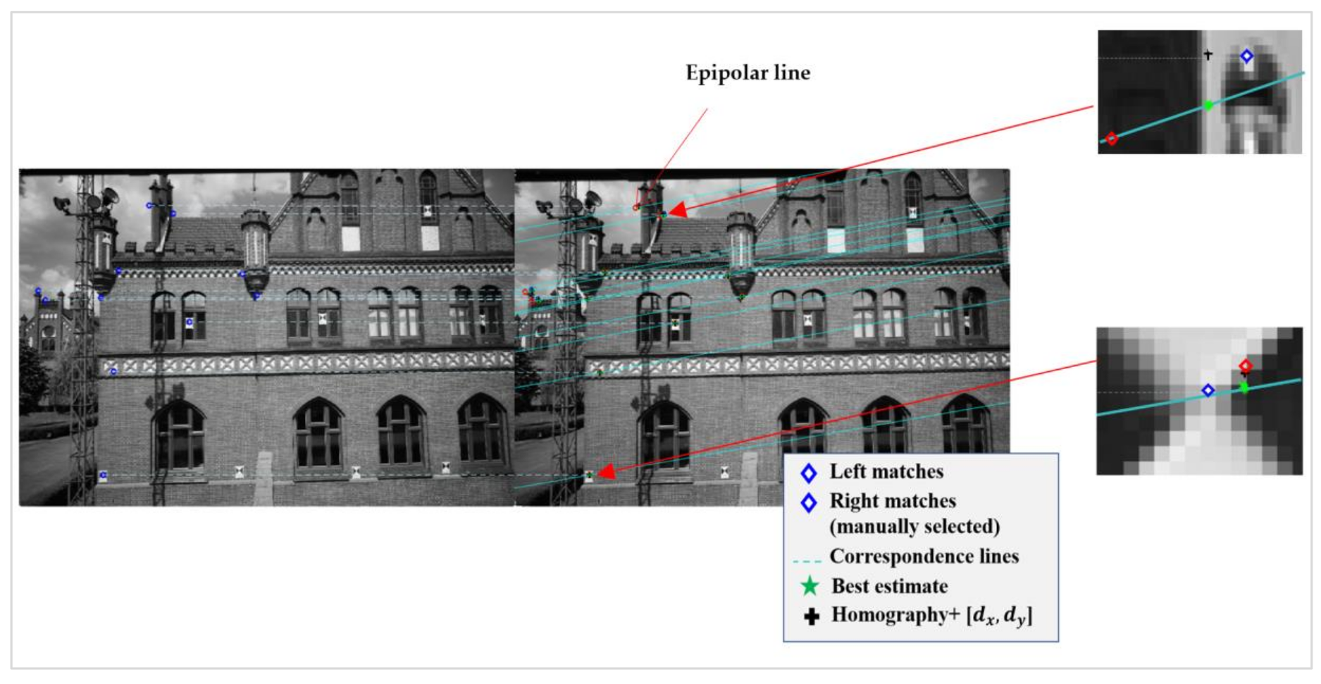
2.1. Epipolar Geometry

Only the ordered pairs ( q , p ) Q × P associated with m q , p   M Q P are governed by the epipolar constraints that are expressed in terms of the epipolar lines   l q , l p and the fundamental matrix   F . Consider that the global homography H is being computed using the matched features, which, generally speaking, cannot be used to relate all of the matched pairs ( q , p ) . This is because homography defines a plane-to-plane relationship, which is not always the case for a pair of images. For now, suppose that the homography relationship holds with an acceptable error tolerance.
If q and p are written in homogenous coordinates as:
q = [ q x ,   q y ,   1 ] T   a n d   p = [ p x ,   p y ,   1 ] T
Therefore, the homography relationship is approximated by:
p H q
Moreover, the epipolar constraint is also approximated by:
p T F q 0
The lens distortion and other noise factors are not considered for the time being.
In the case of a plane-to-plane relationship, the homography and the fundamental matrix are related by [26]:
F [ e r ] × H
where e r is the epipole of I r , and the bracket [   ] × denotes the vector’s skew-symmetric matrix form.
While the homography defines a bijective relation—that is, a one-to-one mapping from I l to   I r —the epipolar constraints define a one-to-many relation, in which a feature point p in I l is mapped to the epipolar line l p in   I r . However, the homography is not an accurate relation, unless all of the features are confined on a plane.
Two remarks should be mentioned regarding the fundamental matrix and the homography. First, despite the theoretical fact that F should be unique, up to a scale factor, for a pair of images, it was found to be sensitive to the distribution of the matched features. Therefore, different forms of F can exist, introducing what is called model degeneracy. The quality of the fundamental matrix is a function of the distribution of the feature points over the scene structure. The fundamental matrix estimated from non-uniformly distributed correspondences could be degenerate, and might result in flawed rectification parameters. It is therefore intuitive to think that the fundamental matrix could be enhanced by adding more evenly distributed matches over different depths or planes in the scene.
Second, consider the case in which I l and I r contain multiple depths, or more generally multiple planes. The global homography   H in Equation (2) cannot be used to retrieve the correspondences of features accurately. Since a homography defines the relation between corresponding points on a plane, different planes in the scene possess different local homographies. This fact inspired Chen et al. to replace the global homography by a set of local planar homographies [5].
It is evident that a correct or an ideal fundamental matrix defines an accurate relationship (constraint) between the features in one image and their corresponding epipolar lines in the other image. On the other hand, global homography does not in general define an accurate relationship between corresponding features. However, local homography, if it could be found, can bring accurate and more informative constraints between corresponding features. Hence, it is valuable to find a local homography for each plane in the image pair. In this paper, instead of finding a set of local homographies h j , we find a set of discrepancy vectors D j as an alternative.
To find the relationship between the local homography   h j   and the discrepancy vector D j   , consider Equation (2) applied in the case of a local homography h j , which clearly has more chance with respect to H to properly describe the relation between corresponding points in a small area of the two images. However, bearing in mind that the mathematical relations are still within some approximations, we can replace Equation (2) by:
p i = h j   q i
where q i and p i are the i th matched features in the left and right images, respectively.
Equation (2) should be modified to account for the error that arises in the estimated position of the feature p i when using the global homography. This can be written as:
p i = H q i + D i
where the vector D i represents the discrepancy between the estimated feature p i using the global homography and the correct one, as described in Figure 2. Note that the general assumption for D i in this equation is to be associated with the feature point q i , i.e., the index of D is i , not j . This assumption will be modified later.
To derive the relation between the global and local homographies, at the feature pair ( q i , p i ) , the vector D i is written in terms of the feature vector q i as:
D i = ϵ   q i
where both D i and q i are homogenous vectors, and ϵ is a matrix that is not strictly unique. Therefore, Equation (6) can be written as:
p i = H   q i + ϵ q i = ( H + ϵ )   q i
Comparing Equation (5) with Equation (8), it can be concluded that the local homography can be approximated mathematically at the feature pair ( q i , p i ) by the global homography H plus an error matrix ϵ :
h   = H + ϵ
From Equation (8), the approximation of the local homography using the matrix ϵ should be valid only at the feature pair ( q i , p i ) . Actually, ϵ might change dramatically over the same surface represented by the local homography h   , especially in cases where that surface is not facing the camera. Moreover, ϵ   does not have to be unique, as from Equation (7), the entries of ϵ can be chosen arbitrarily as long as the equation is valid. Consequently, instead of computing the local homography from Equation (9), it is more practical to estimate the discrepancy vector D i corresponding to the pair ( q i , p i ) and use it in Equation (6) to find an approximation for the feature p i .
The important question now is whether we must estimate a discrepancy vector D i for each feature pair ( q i , p i ) , or we can assign a single discrepancy vector D j   to a set of neighbouring features. In the situations in which the image contains a dominant planar surface facing the camera, as in Figure 2, it can be assumed that one discrepancy vector is approximately constant over a single surface. Therefore, the assumption that there is a one-to-one correspondence between D j   and h j   is relatively valid. It is then enough to find the set of discrepancy vectors as a representation of the local homographies.
Now, consider the general case of multiple planar surfaces, each of which is of a different orientation. Take for example images that are taken for indoor environments. In this case, the discrepancy vector is point-dependent, rather than plane-dependent, i.e., D i changes with ( q i , p i ) . However, as an approximation, it can be assumed that the vector D i   is locally constant for the feature points that exist in the vicinity of ( q i , p i ) . It will be discussed in Subsection 2.2 how the vector D can be assigned to a set of feature pairs in the neighbourhood of ( q i , p i ) using the kD-tree data structure.
That is, for any feature point q i in I l   , the corresponding feature point p i is determined by applying the global homography H and adding the discrepancy vector D j .
Now looking at Equation (3), due to image distortion, errors in camera calibration, and image noise, the epipolar constraint will be perturbed by a small value arising from such errors. Hence, the mathematical model in Equation (3) should be modified to account for these errors. The error term   is added, such that Equation (3) becomes:
p T F q =
The term F q represents the epipolar line in   I r Thus, we can write Equation (10) as   p T l p = , which can be expanded as:
a r p x + b r   p y + c r =  
where l p = [ a r , b r , c r ] T . Equation (11) states that the feature point p lies approximately on the line l p with an error   . Therefore, for each detected feature q in   I l a corresponding epipolar line l p is approximately determined. However, we seek an approximation of the corresponding feature point p rather than l p .
The approximation of p ( p x , p y ) can be determined from Equation (11) with the combination of another equation, if there is any. Let’s consider that p x is known and fixed; then, we can write:
p y = a r p x c r b r
The question now is how to fix p x . Utilising the global homography and the discrepancy vector, we can have an estimate of the feature’s location from Equation (6), which is denoted p H . The estimation of p H from Equation (6) might not be very accurate. Therefore, to reduce the total error in p H , we could estimate only p x using Equation (6), and then use Equation (12) to approximate p y . In other words, we are projecting the point p H on the epipolar line l p in order to find a more accurate feature point denoted p F   (i.e., we are not relying on the homography to estimate both p x and p y ).
Before proceeding with the proposed methodology, it is good to expand the discussion of the errors associated with the estimation of both the homography and the fundamental matrix. Consider the set of unfiltered matches G u v such that   M Q P G u v , Q U and P V where M Q P is the set of all possible correct matches.
Obviously, the size of M Q P expands and diminishes based on the filtering criteria. Let’s consider that the matches are being filtered with RANSAC, or one of its variants, by fitting either a fundamental matrix or a homography. To expand M Q P , it is required to relax the distance threshold of the global homography model; however, that comes with the price of inclusion of outliers amongst the inliers. The fundamental matrix model, on the other hand, tends to have more accurate matches.
Figure 3 shows a comparison of the errors and number of matches between two of the models for a pair of test images. It is evident that more matches are included in the homography model, but with less accuracy.
The examination of the estimated global homography in the example above shows that it represents the relation between points on the predominant building façade. Other points off that building façade would have a discrepancy vector [ d x , d y ] T from the model. The discrepancy vector D can be written in terms of d x and d as:
D [ d x , d y , 1 ] T [ ( ( H q ) x   p x )   , ( ( H q ) y p y )   , 1 ] T  
As might be expected in the above example, D is almost zero for points on the building façade, and has larger values for off points. Figure 4 shows the discrepancy profile for the matches of the test image used in the above example. It can be seen that the profile resembles the different depths in the test images, with zero discrepancy for the points on the main building façade.
Now, back to the problem of fixing either p x . If we can build a prior profile for   D , we could approximate   p x using Equation (13).
p x can be approximated by:
p x [ H q ] x + d x
Equation (12) is then used to find p y .
To summarise the geometrical approximation, we first estimate the location of p H given   q using the global homography and the discrepancy D , and finally project the point p H on the epipolar line l p in order to find a more accurate location of the point p F .
To examine the accuracy of the geometrical approximations, a set of random features in I l were manually selected with their true correspondences in I r . These correspondences are again computed using the geometrical constraints. Subsequently, the error is computed using the manually selected features’ locations in I r as a reference.
Figure 5 is a visualisation of the error between different geometrical approximations of p and the reference. The numerical comparison is demonstrated in Figure 6. From the two figures, it can be seen that the error in the final approximation is less than 10 pixels for p x and   p y . This might not be the case in all situations, but it shows that an acceptable initial approximation of the correspondences’ locations can be obtained using the epipolar constraints.
It might seem from Figure 6 that the error is less before projecting the feature points on the epipolar line. However, when a better estimate of the fundamental matrix is obtained, the accuracy of epipolar projection should be improved.
To this end, we have seen that the homography and epipolar geometry could be used to find an initial approximation of the features p i in I r , which corresponds to the selected features q i in I l , provided that a discrepancy profile exists; that is, all of the discrepancy vectors D i are known. The question arising now is how to estimate and assign a discrepancy vector D i to the feature p i . In the next subsection, we demonstrate how initial matches are used to estimate and assign the vector D i for newly detected feature points p i .

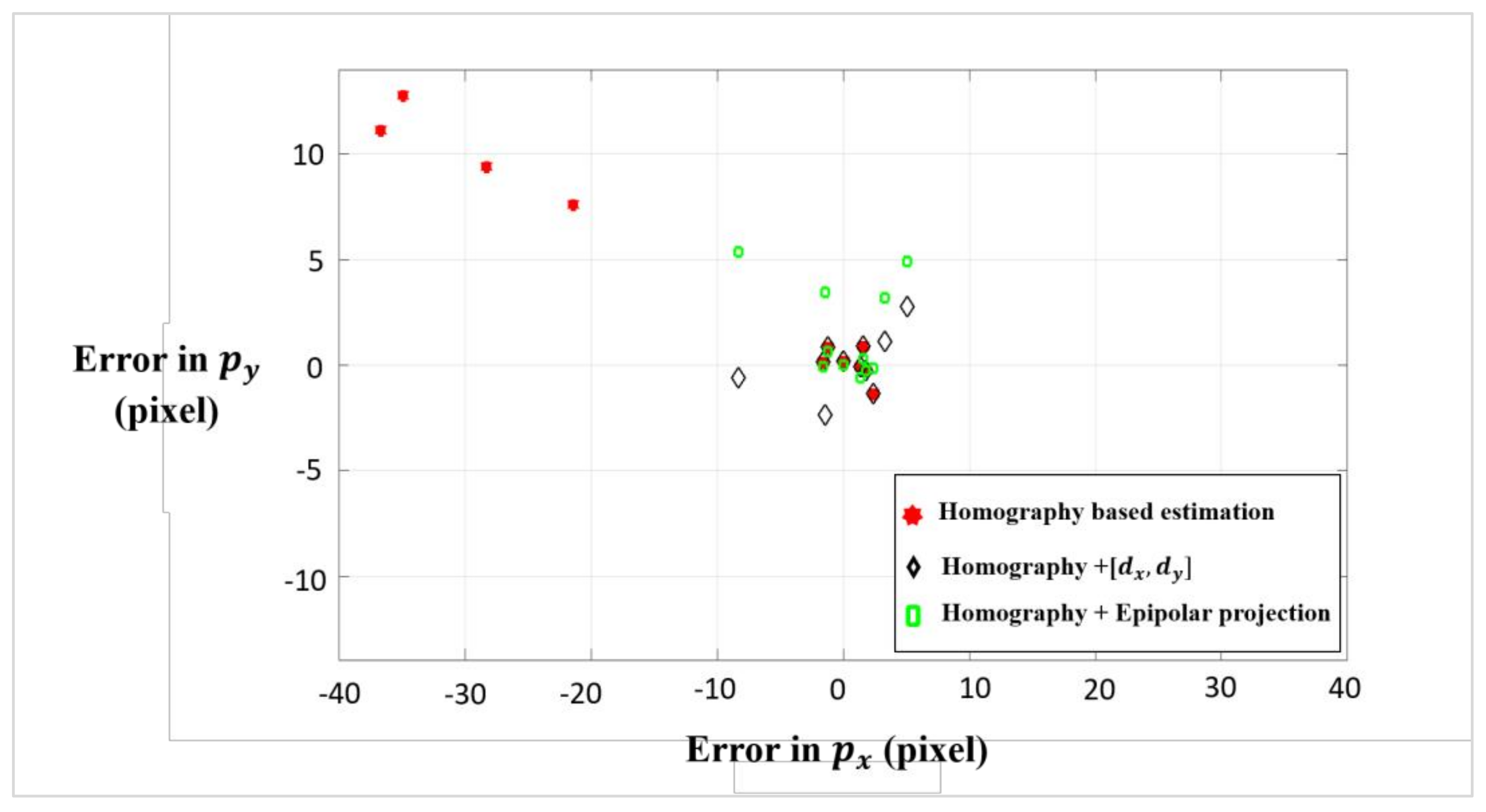
2.2. Discrepancy Assignment

Let the seed of matches be S   = { ( q , p ) | ( q , p ) Q × P ,   m q p M Q P } and let the initial set of discrepancy vectors be   Δ = { D i | i + , D i 2 } . An initial discrepancy vector D i is defined as in Equation (13). Where a homography is computed from all of the elements of S   , then D i is computed as the difference between H q i and p i . Now, each pair ( q i ,   p i ) is associated with one vector   D i Δ . However, each vector D i can be assigned to one or more pairs ( q j ,   p j ) .
If a feature point u in I l is in the neighbourhood of q i , this implies that its corresponding feature point v is also in the neighborhood of   p i . Then, we can safely assign D i , which is associated with ( q i ,   p i ) , to ( u , v ) .
Now, the task of checking whether each detected feature point is in the neighbourhood of ( q i , p i ) S or not is time-inefficient. Instead, for each   ( q i , p i ) S associated with D i , we find a set of neighbouring points N q i p i in the neighbourhood of ( q i , p i ) . Each element in N q i p i   is an ordered pair and is assigned the vector D i . The set of feature pairs ( u , v ) in the neighbourhood of ( q i , p i ) is:
N q i p i = { ( u , v ) | u q i ρ l ,   v p i ρ r }
where ρ l and ρ r   are the distances between two features in I l and I r , respectively.
To speed up the neighbourhood search and assignment, we organise the feature points in I l and I r using the kD-tree data structure [27]; then, we perform a range search to find the neighbourhood of feature points for each element in the seed, such that each element in the seed is assigned a set of neighbouring feature points.
It is important to note that some of the neighbouring features ( u j , v j ) might belong to a different plane from that of the pair   ( q i , p i ) , which results in the inaccurate assignment of   D i . These points will be either corrected by the template matching or discarded if no correlation peak is found.

2.3. Feature Detection

The detection of features in I l is achieved using the well-known FAST detector, as it is time-efficient and easily implemented. FAST checks whether a point q is a corner or not by comparing its intensity Z q against its circle of neighbours. q is considered a corner if it is surrounded by points that are all brighter than Z q + σ or darker than Z q σ . σ is a certain chosen threshold, and the circle size could be chosen as of eight , 12 , or 16 pixels. A speed test can be performed over a fewer number of pixels for the fast rejection of non-corner points, using the nearest five, seven, and nine pixels. That is, there are different versions of the FAST detector, namely, FAST-5, FAST-7 and FAST-9, all of which are dependent on the single parameter   t . Normally, multiple adjacent features are detected, which is an issue that requires non-maximal suppression to be applied on the set of detected features. The FAST detector is well documented, and more details about the FAST feature detector can be found in the work of Rosten et al. [18,28].

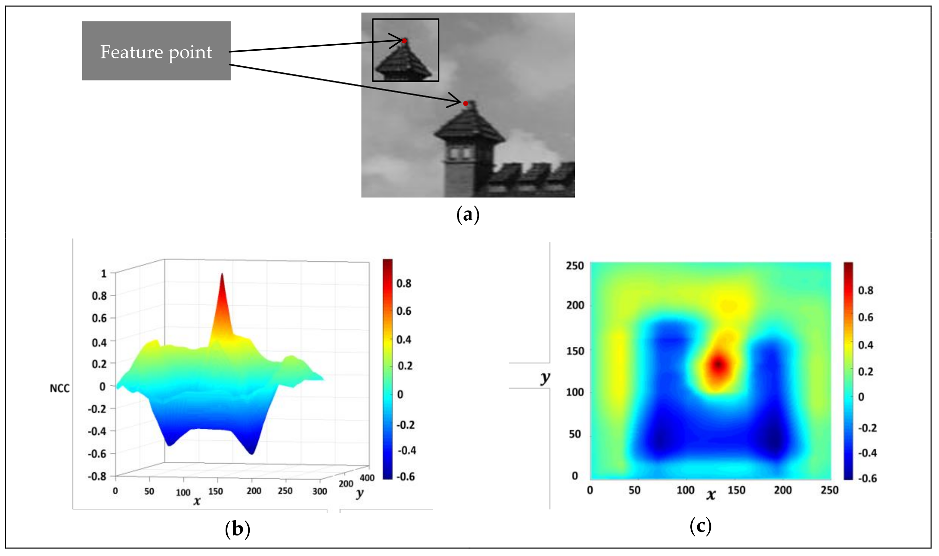
2.4. Template Matching with Normalised Cross-Correlation

As discussed in the previous subsections, geometrical constraints can predict to a certain accuracy the location of a feature point p i in I r   corresponding to a selected feature q i in   I l . In most cases, that prediction of p i is not correct and differs from the actual pixel location by a shift   ( δ x , δ y ) . Consequently, template matching is utilised to correct the pre-estimated location of p i .
There are several reasons for choosing template matching over descriptors when matching features. First, template matching does not require the computation effort required when matching via descriptors. Second, the time required for template matching is reduced, since the search image is now limited to a small region around the predicted feature p i . Moreover, matching time could be further reduced if an image pyramid is used. Furthermore, in most cases, template matching avoids mismatches, as the measuring score is maximum at the point of exact concurrence, leading to more deterministic results than those obtained by the descriptors. Finally, it will be shown that affine transformation can be applied to the template to cope with the affinity of the search image.
Template matching was defined by Goshtasby [29] as the process of determining the position of a subimage called the template t ( x , y ) inside a larger image called the search area s ( x , y ) . In other words, the template window slides over the image or region of interest and a score is calculated, which is its maximum at the location of exact concurrence. An example of template matching is depicted in Figure 7.
The matching score could be the summation of absolute difference, the summation of squared difference , or the NCC. These are the most common scores used, while there are other scores used in the literature [30].
In this paper, NCC is used because it is robust to illumination changes. NCC is defined as [31,32]:
γ u , v = x , y   ( s ( x , y ) s ¯ u , v ) ( t ( x u , y v ) t ¯ ) x , y   ( s ( x , y ) s u , v ) 2 x , y ( t ( x u , y v ) t ¯ ) 2
where s ¯ u , v and t denote the mean of s and t within the area of the template, respectively. NCC in this form is too expensive to compute. Lewis [33] proposed the use of recursive summation tables of the image function to find an approximation of the numerator and denominator of γ u , v .
It was shown by Lewis [33] that the fast NCC could reduce the time of matching dramatically. Furthermore, if fast NCC is considered over a small region of interest, just like in our case, it is expected to give satisfactory results in a short time.
The main drawback of template matching is that it does not provide a subpixel accuracy by itself. However, this issue can be solved by using techniques to find matches to the subpixel accuracy. One of the techniques that is used is to fit a second-degree surface to the correlation coefficients and find its extrema [34].

2.4.1. Window Size Optimisation

The sizes of the template and the source image should be adequately selected to trade off the time efficiency with the accuracy of matching. The template size can be chosen as a small number of pixels around the feature point, such as for instance 9 × 9 or 15 × 15. Adjusting the size of the source subimage is the most significant to the mitigation of matching time. The source image must be selected around the approximated location of the feature p i in   I r . If the subimage’s size is too small, it might not include the correct feature, and if it is too large, it will be time-inefficient. Hence, a two-step approach is proposed to select the size of the subimage properly. First, the size of the subimage can be related to the discrepancy vector D i . As this vector indicates the deviation of a feature p i from the estimated homography, it also reflects the uncertainty region in which an approximated point p i is in the vicinity of the exact feature point   p ^ i . Therefore, we can initially set the size of the source subimage to (2 d x   + 1) (2 d x   + 1) or simply (2 d x   + 1) (2 d x + 1). Second, to further optimise the NCC time, instead of sliding the template over the whole source image, only small subimages over the regions containing the features p can be selected, and the NCC is computed over these subimages as small source images. Figure 8 shows that a source image may contain a large area of no features. Consequently, it is time-consuming to include the whole source image when performing NCC.

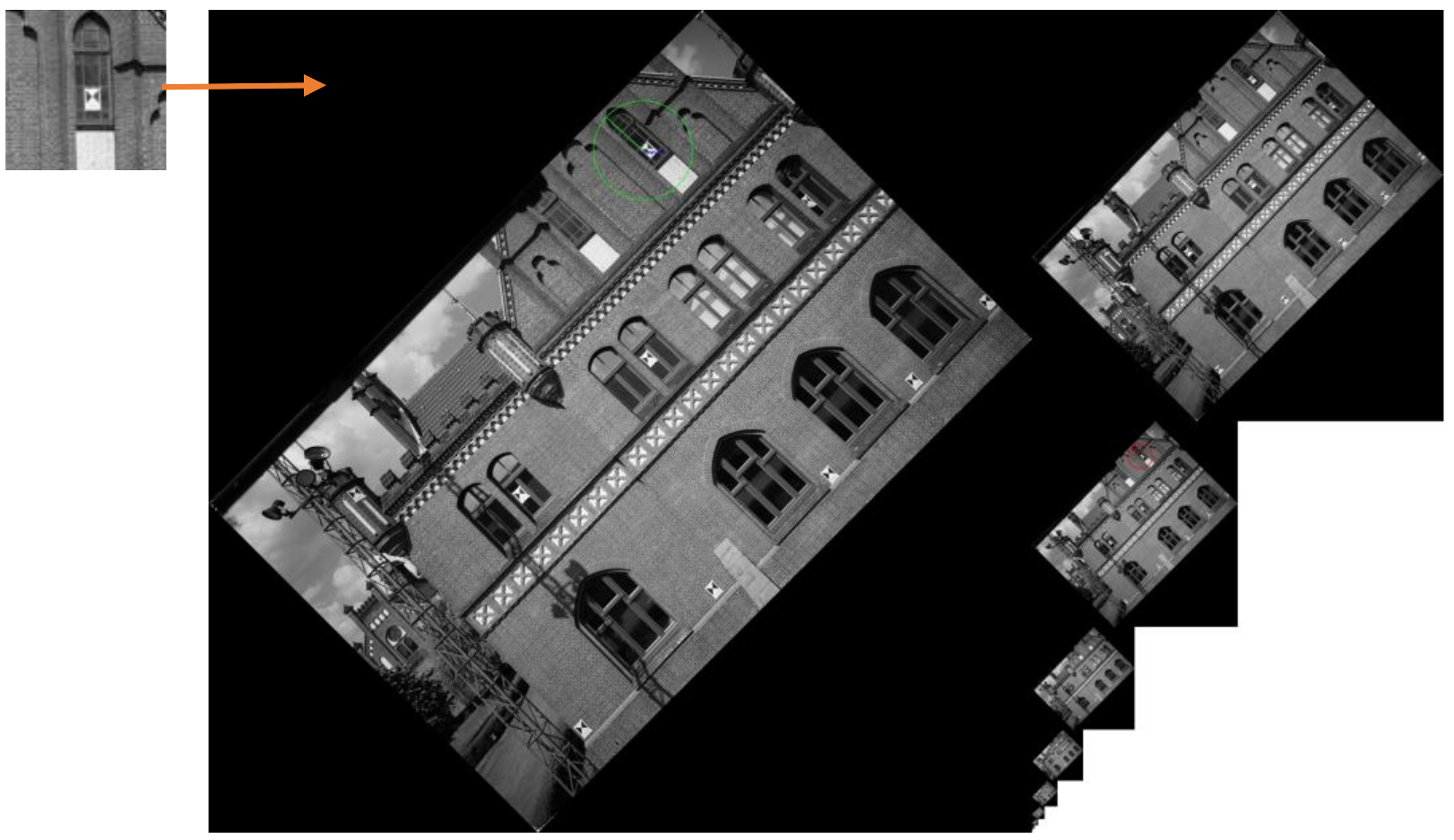
2.5. Scale and Orientation Assignment

In matching pairs of images of different scales, orientation, or both, NCC does not perform accurately unless the rotation and scale of one image, relative to the other, are estimated and applied to the template. Utilising the homography H , which is computed from the initial matches of the seed S , we can compute the orientation and scale of I r with respect to   I l . Then, we can recursively enhance the homography by adding more accurate matches, which in turn enhances the accuracy of the estimated rotation and scale.
Assuming the homography defines a projective transformation between the two images, which is the general case, SVD is used to extract the rotation angle and the scale from the homography. Furthermore, we can derive other affinity properties, such as the deformation angle.
The homography H can be written as [35]:
H = [ A t V T v ]
The affine properties are contained in the matrix A , which can be decomposed as:
A = R ( θ ) R ( ϕ ) W   R ( ϕ )
where R denotes the rotation matrix, θ and ϕ denote the rotation and deformation angles, respectively, and W is a diagonal matrix containing the scaling parameters.
W = [ λ 1 0 0 λ 2 ]
In most applications, λ 1 λ 2 . That is, the transformation tends to be a similarity. However, even in the case when λ 1 λ 2 , the template could be modified to cope with the transformation.
Using SVD as in Hartley et al. [35], we can express A as:
A   = U W V T = ( U V T ) ( V W V T ) = R ( θ ) ( R ( ϕ ) W   R ( ϕ ) )
where U and V are unitary matrices, and W is a diagonal matrix with non-negative entries. In the current special case of A being a 2 × 2 matrix, the matrices U ,   W , and V are of the same size as A .
Therefore, the procedure to compute the rotation angle θ starts with decomposing   A , and then setting   R ( θ ) = U V T . Afterwards, it is straightforward to find   θ . Similarly, the scale and the deformation angle could be easily retrieved.
The next step is to apply the rotation and scale to the template before performing template matching. This approach of assigning global rotation and scale to the whole image is much faster than assigning specific orientation and scale to features via descriptors.

2.6. Seed Initialisation

It was decided to discuss the formation of the initial seed of matches in this subsection, as it is mainly achieved through template matching. In most cases where the images that make up the pair have approximately the same orientation and scale, template matching via NCC is used to retrieve the correspondences in the image I r   for some of the selected features in the image I l . First, the two images are scaled to a proper smaller size. The scale is chosen according to the initial resolution of the image pair in order to speed up the matching time and preserve the quality of matching at the same time. The next step is to detect the strong features in I l   using FAST. Then, a smaller subset of these features with well distribution over I l is selected. For each feature in I l , the corresponding feature in I r is found using NCC.
In other cases where there is a difference in scale, orientation, or both between the image pair, the Ciratefi method [25] could be employed to find the initial set of matches, as well as the scale and rotation angle. Ciratefi is composed of three filters: the first is Cifi, which stands for “Circular Sampling Filter”; the second is called Rafi, which stands for “Radial Sampling Filter”, and the last is called Tefi, which stands for “Template Matching Filter”. The first filter determines a proper scale; the second detects a probable rotation angle, and the third is a typical template-matching filter. An example of Ciratefi with rotated images is shown in Figure 9.
Experiments on Ciratefi proved its high accuracy; however, the only drawback is the slow performance compared with regular template matching. There are a few techniques to shorten the time of Ciratefi. For example, for images with no projective distortion, the scale and rotation angle for only one feature can be obtained using Ciratefi, and then regular template matching is used after applying the scale and rotation to the template image.
In both scenarios, a set of well-distributed matches is found. These matches are then used to compute the initial homography and fundamental matrix.

2.7. Summary of the Proposed Methodology

Figure 10 and Figure 11 present an overview of the proposed methodology. Figure 10 describes the geometric approximation of point correspondence. As discussed earlier, we begin with template matching to find a seed of matches to estimate an initial homography H and an initial fundamental matrix F . To generalise, we use Ciratefi for template matching unless there is a prior knowledge about the scale and orientation, in which case regular template matching is used. As template matching can generate an accurate set of correspondences, the homography and fundamental matrix can be estimated directly. We then use H to generate a set of discrepancy vectors D i and assign them to each matched pair ( q , p )   . Next, we perform the k d-tree range search to find a neighbourhood of features N i for each pair   ( q , p ) i . The search is performed over a set of features, which are detected only once via FAST feature detector. The vector D i is then assigned to each neighbourhood of points   N i , such that a discrepancy profile is created for all of the newly added feature points in I r . Using the discrepancy profile and the epipolar lines, we can geometrically find an approximated location for each feature point p i corresponding to a feature   q i .
Figure 11 describes the general methodology in which the seed is recursively extended. The geometric approximation of matches is then applied for each approximation, and template matching is employed to correct the locations of the features p i . To limit the result to accurate matches only, feature points with NCC scores of less than   0.9 are rejected. Accurate matches are then added to the seed, and the matrices H and F are recomputed.
The process in Figure 11 is recursively repeated until the set of FAST features is covered. It is expected that not all of the features that are detected by FAST be matched, but rather only a subset of them, as some of the features in the left image do not have correspondences in the right image, or might have small correlation scores.
The proposed method tries to find matches that are well-distributed over the overlapping area and the different depths of the image pair, and that are governed by the epipolar constraints.

3. Results and Discussions

3.1. Experimental Dataset

The proposed methodology was tested using two datasets. The first dataset was provided by the International Society of Photogrammetry and Remote Sensing (ISPRS) through the ISPRS and EuroSDR benchmark on multi-platform photogrammetry [36]. This dataset is for the Zollern Colliery (Industrial Museum) in Dortmund, Germany. The images in this dataset were taken by an unmanned aerial vehicle (UAV) in a close-range manner. Several images with different characteristics are used from this dataset to test the proposed methodology. The images used from this dataset are intentionally selected based on the relative geometry between the image pairs to examine the projective distortion, large baseline, and the variation in scale and orientation. Therefore, some images are not in the same chronological order as when they were taken by the UAV. In practice, successive images are processed together in order to obtain accurate results. However, this is not always the case in the following experiments.
The other dataset contains one image pair taken by a mobile camera for an indoor environment. The images were taken by the rear camera of a Samsung Galaxy Note-3, model number: SM-N900W8 (Samsung Electronics Co., Ltd., Suwon, Korea). Images were taken inside one of the engineering buildings at the University of Calgary, Canada. The images in this dataset were taken by an uncalibrated camera. Furthermore, the images contain several planar surfaces with different directions, such as the roof and the walls, and few non-planar objects. So, this dataset provides a challenging scenario for testing the method with multiple local homographies.
Table 1 lists the image pairs used with their properties. The first image pair is from the ISPRS dataset, and is characterised by a predominant building façade with multiple depths in the background. The second image pair is for the same building façade but with a relatively larger baseline and more scene structure in the background. The third image pair exhibits a different orientation of the camera from the left image to the right one. The fourth image pair is the same as the first image pair, but with different scale and orientation. Lastly, the fifth image pair is for the dataset taken by the smartphone, to emphasise that the method can find good matches even in challenging situations.

3.2. Evaluation Criteria

Visual and numerical indicators are used to evaluate the proposed method and compare it with other state-of-the-art methods. In most cases, the number of the correct matches obtained by the proposed method is large enough compared with the number of outliers. This allows solving for the fundamental matrix via LS, with the option of using outlier rejection techniques if required. The proposed method competes as a single procedure against the block of procedures consisting of a descriptors assignment, preliminary matching, and RANSAC. Therefore, it is being compared with SIFT, SURF, and ORB before and after their matches are filtered with RANSAC.
Two numerical indicators are used in each of the experiments after filtering the data. The first is the Percentage of Correct Matches to the Features’ number (PCMF). The second indicator is the Matching Precision (MP) which is based on the Number of Precise Matches (NPM) and was adopted by Chen et al. [37]. MP is defined as MP = (NPM/M) × 100%, where NPM are obtained after filtering the data with RANSAC, and M is the number of all of the matches. The precision of matches is the key to determining the quality of matching when neither ground truth nor an accurate fundamental matrix model exists. On the other hand, accurate matches are only determined if ground truth or an accurate fundamental matrix is obtained from orientation sensors.
For convenience, the number of detected features is approximately fixed in each method to neutralise the effect of the feature detection step when evaluating the matching process. The number of features was controlled by tuning the thresholds in each method except in SIFT, in which the images were resized instead, as SIFT exhibits slow performance when dealing with large images.
To judge the correctness of the matches of each method, the reprojection error is computed using the known camera matrices of the images. Then, an error threshold of less than 1 pixel is used to reject incorrect matches, i.e., matches are considered correct if their reprojection error is less than one pixel, and are considered incorrect otherwise. Hence, another indicator is involved, namely, the Matching Accuracy MA = NAM/M, where NAM is the Number of Accurate Matches. The camera matrices for the third pair in Table 1 are not reliable, as there is a time gap between the left and the right images, which might lead to inaccuracy in the external parameters, especially those obtained from inertial navigation sensors (INS). Furthermore, the experiments on the third and fourth image pairs in Table 1 are performed to depict the ability of the proposed methodology to work with pairs of different scales and orientations. Therefore, the accuracy measure is limited to the first and second image pairs only. Consequently, the number of correct matches is defined as the number of accurate matches in the tests performed on the first and second image pairs, and defined as the number of precise matches in the tests performed on the other image pairs.
The results of the experiments are presented in Figure 13 through Figure 18 in terms of the precise and accurate matches. Additionally, Figure 20 shows the disparity maps computed for the fourth image pair, which can be considered as another quality measure of the feature matching.

3.3. Matching Performance

The proposed method was tested on the image pairs that are listed in Table 1. The results are depicted numerically and visually in Table 2, Table 3, Table 4, Table 5 and Table 6 and Figure 13, Figure 14, Figure 15, Figure 16, Figure 17 and Figure 18, respectively.
The matching precision and accuracy of the proposed method are high compared with the other methods. Similarly, the percentage of correct matches to the number of features is higher in the proposed method than in the other methods. This is especially true in comparison to ORB, which shares the same feature detector as the proposed method.
Histograms were plotted for the reprojection errors of the first and the second image pairs. The reprojection error is defined as [35]:
E i = d ( q i , q ^ i ) 2 + d ( p i , p ^ i ) 2 )
where   ( q i , p i ) are the matched pair, and q ^ i and p ^ i are the reprojected points in the left and the right images, respectively. The term d ( q i , q ^ i ) denotes the Euclidean distance between q i and q ^ i . By definition, the reprojection error is positive, so the histogram is one-sided starting from E i = 0 .
The histograms of the errors are used to determine the threshold at which the matches are rejected. It was found that the majority of the errors are less than one pixel; therefore, this value was chosen as a rejection threshold for the incorrect matches. Another advantage of the histograms is that they show the upper bound of the errors associated with each method. In the following histogram graphs, the intervals of errors are limited to [0,5], as most of the significant errors are within this interval. This is not always the case, since methods such as ORB might exhibit error instability, as will be shown in the matching test of the second image pair.
The experiment on the first image pair emphasises the difficulty that other methods encounter when matching images of multiple planes or depths. It can be seen that the precise features in the first image pair using SIFT, SURF, and ORB are only concentrated on the main building façade, with very few features or none on the other depths of the image pair. This is a result of using RANSAC, which tends to find a degenerate model of the fundamental matrix that is different from the ideal one. It is clear from Table 2 and Figure 13 that the number of precise features is small compared with the number of accurate features, except for the proposed method. It implies that using RANSAC is harmful, in some cases, to the accurately matched features. PCMF indicates the effectiveness of the detect-and-match strategy, as the number of correct matches compared with the detected features is relatively large in the proposed methods. Furthermore, although the histograms in Figure 12 are limited to the interval [ 0 , 5 ] , the upper bound of the reprojection error in the proposed method is 25 pixels, while it reaches 656 pixels in SIFT, and thousands of pixels in SURF and ORB. The upper bound of the reprojection errors can be represented by their standard deviation, which is very small in the proposed method compared with the other methods. These results support the outliers in the proposed method being constrained to be within small distances from the correct correspondences. Therefore, direct LS can perform well in estimating the fundamental matrix, since the effects of those constrained outliers are insignificant.
The second image pair is characterised by a large baseline as well as multiple planes, depths, and scale variation. Similar results to the first test are depicted in Table 3 and Figure 15, except that the PCMF is lower in this test than that of the first test, which is a result of the smaller overlap and the change in geometry between the image pair (i.e., scale and depth). The experiment on the second pair proves the capability of the proposed methodology to work with multiple local homographies that are different from the global homography.
The histograms of the errors in Figure 14 follow the same pattern as in the test of the first image pair, except that the error range is now larger due to the less overlap and the geometry difference between the image pair. The errors associated with the ORB method seem to be the worst, as the frequency of the errors is significant even at errors of 80 pixels.
The experiment results for the third and fourth image pairs exhibit high geometrical distortion. These image pairs are selected to examine the robustness of the proposed method to variation in geometrical properties, such as scale, rotation, and projectivity. The PCMF and MP in Table 4 and Table 5 indicate the higher performance of the proposed method compared with the state-of-the-art methods. The matching performance is also depicted in Figure 16 and Figure 17. As expected, ORB is of low performance in both cases. Again, it should emphasised that although ORB uses a modified version of the FAST detector to account for the rotation and scale, the proposed method outperforms it significantly. In other words, robust and accurate matches can be obtained based on relatively weak detectors.
The fifth image pair is chosen to test the proposed method in challenging scene structures. The image pair contains planes with different orientations and without a single predominant planar surface. Comparison of the results in Table 6 indicates the notable performance of the proposed method. Furthermore, the results in Figure 18 reflect the better distribution of the matches obtained by the proposed method than those obtained by SURF and ORB. In the next subsection, a demonstration of the impact of the matches’ distribution on the disparity map is presented.
The test results prove the accuracy and robustness of the proposed method over the state-of-the-art methods. However, some matches are rejected by the proposed method as well as other methods. The rejected matches of the proposed method are relatively close to the correct matches’ locations. Thanks to the geometrical prediction step, the outliers are close enough to the correct matches. This allows using the matches with a LS adjustment to estimate the fundamental matrix. On the other hand, when dealing with other methods, besides being of a large number, the outliers usually are inconsistent, such that LS fails to find a correct fundamental matrix. Hence, RANSAC is employed to filter those outliers, but in many cases, it finds a degenerate model of the fundamental matrix.
Furthermore, in some applications, it might be desirable to detect matches that are within a few pixels of the correct matches, which make the proposed method more favourable than other methods.

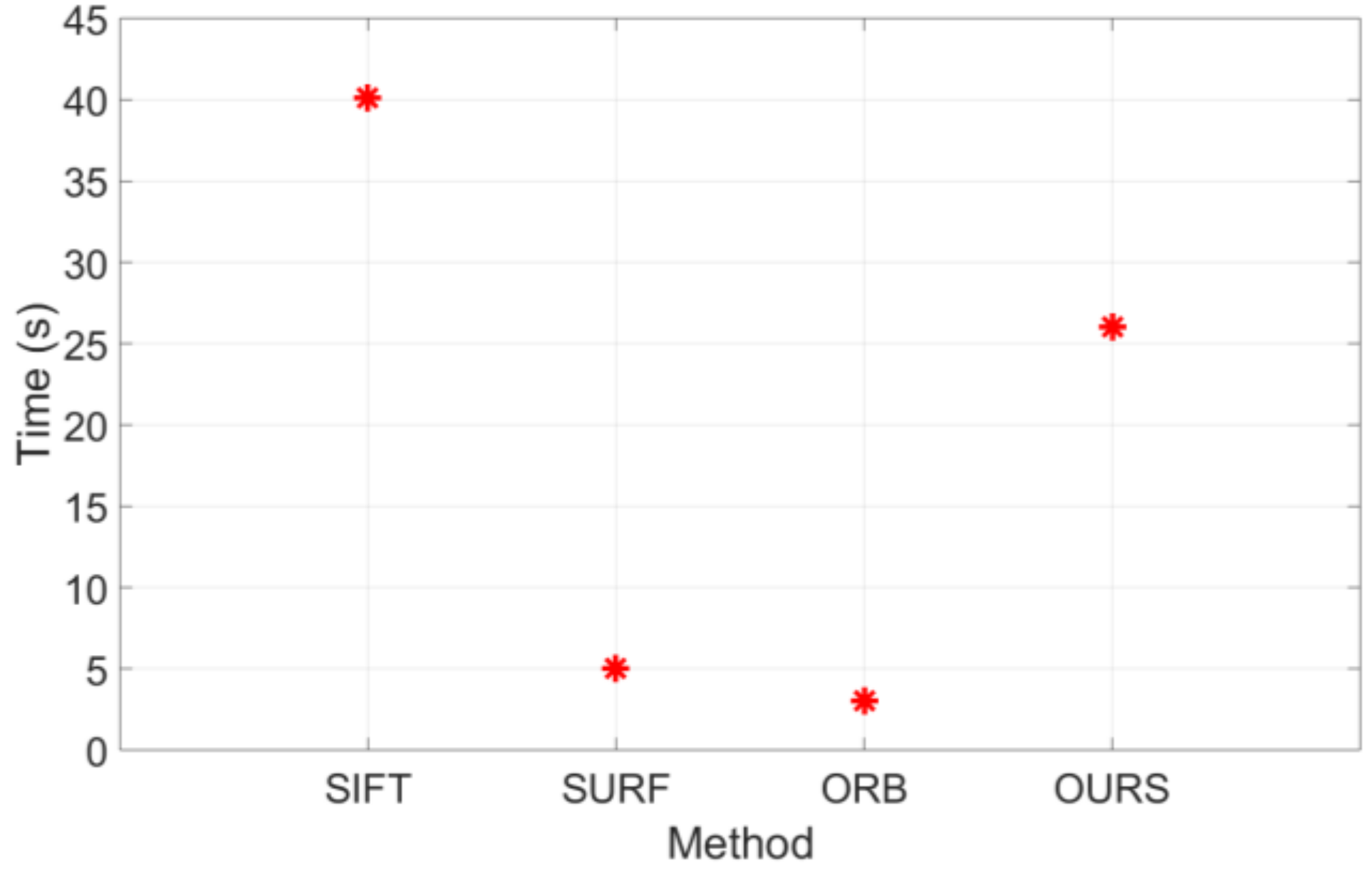
3.4. Processing Time

The average processing time of the state-of-the-art methods, including RANSAC processing time, versus the proposed method, was calculated in seconds for the first image pair. Figure 19 shows a comparison of each method’s processing time. It is worthwhile to mention that although the tests were performed on the same machine, the implementation of the proposed method is not optimised for parallel computing, which should mitigate the processing time dramatically. The code for SIFT was obtained from Lowe’s website. It was implemented in C language, but has MATLAB calling functions. The MATLAB built-in functions were used for SURF, while ORB was implemented using a C++ code with the OpenCV library. Therefore, only SURF and the proposed method were implemented with MATLAB code, which is known to be slower than C/C++ codes.
Hence, the proposed method is a tradeoff between accuracy and efficiency, but at the same time can be optimised for better time efficiency.

3.5. Applications

As discussed earlier, the uniformity of feature matching is significant to the estimation of a non-degenerate fundamental matrix and other feature matching-dependent applications, including sparse point cloud generation.
A noise-free sparse cloud can be obtained by photogrammetric intersection (triangulation) if there exists an outlier free set of matches. However, accuracy is not the only factor impacting the quality of the generated point cloud, but also the distribution of the feature points. For example, the concentration of the feature points around a specific region, may result in significant gaps in the constructed scene, especially when such behaviour is repeated in several pairs of images.
Dense matching is another example in which the distribution of feature points is critical. The process of dense matching typically starts with the selection of a set of matches, followed by the estimation of both the fundamental matrix and the rectification parameters. Then, if two images are correctly rectified, the search for point correspondence on epipolar lines is straightforward. The errors in dense matching are due to either illumination and other radiometric properties of the stereo pair, or to a flawed rectification. Thus, to limit the errors of dense matching to only the radiometric errors, we must obtain a well-rectified image pair, which is dependent on the estimation of the fundamental matrix. We have seen earlier that the estimation of the fundamental matrix is a function of the distribution of matches over the overlapping area of the image pair.
The effect of the distribution of matches on the sparse point cloud generation is evident from Figure 13 and Figure 15. In Figure 13b,c, very few points are in the background, and most of the points are concentrated on the front building façade. Hence, it is evident that triangulation would lead to a two-dimensional (2D) surface in Figure 13b,c, which is opposite to the case in Figure 13a, in which points are distributed over different scene structures.
Figure 20 highlights the impact of matching methods on the disparity map. Figure 20a,b are the results of dense matching using the fourth image pair after the images are rectified based on the proposed matching method and on SURF, respectively. The disparity map in both cases is computed using the Semi-Global Matching [38]. It is evident that in both images, there exist errors due to illumination difference. Nevertheless, the disparity map in Figure 20a is far better than the one in Figure 20b. The rectification in Figure 20b is affected by more feature points being located on the building façade, which in turn results in an inaccurate fundamental matrix and flawed rectification. As a result, only part of the building seems to be correctly matched, and the rest of the image is noisy.

4. Conclusions

In this paper, a robust uniformly distributed feature matching method is introduced. The method is based on the prediction of corresponding features using the epipolar constraints and the refinement of the correspondences’ locations using template matching. Firstly, a small set of matches is found. For the method to be self-contained, template matching is employed to find this initial set. Either the regular template matching or Ciratefi method, when there are significant rotation and scale differences, is used. From the initial set of matches, the fundamental matrix and homography are calculated. Then, for all of the detected features in the left image, approximated locations of their correspondences in the right image are found using both the local homographies, which are encapsulated in the discrepancy vectors and the epipolar projection. Secondly, template matching is employed with NCC to find more accurate correspondence locations from the approximated ones. The proposed method does not employ descriptors, which is memory and time inefficient, and moreover more probabilistic rather than deterministic. To account for the variation in scale and orientation, SVD is used to find a global scale and orientation for the right image. Scale and rotation are then applied to the template window.
The experimental tests of different images with different characteristics proved that the proposed method is more robust and generates more uniform matches than the current state-of-the-art methods. Furthermore, it solves the problem of model degeneracy at the detect-and-match level, instead of the RANSAC level.
The only apparent drawback of the proposed method is the processing time compared with SURF and ORB. However, processing time can be optimised via parallel computing.

Author Contributions

H.M.M. conceived the approach, developed the software and mathematical model, conducted the experiments, and wrote the manuscript. N.E.-S. initiated the research idea and provided valuable feedback.

Acknowledgments

This project was funded by research grants from the Natural Sciences and Engineering Research Council of Canada (NSERC) and the Canada Research Chair funds of El-Sheimy. The authors would like to acknowledge the provision of the datasets by ISPRS and EuroSDR, released in conjunction with the ISPRS scientific initiative 2014 and 2015, lead by ISPRS ICWG I/II.

Conflicts of Interest

The authors declare no conflict of interest.

References

  1. Moravec, H.P. Rover Visual Obstacle Avoidance. In Proceedings of the 7th International Joint Conference on Artificial Intelligence, Vancouver, BC, Canada, 24–28 August 1981; Volume 2, pp. 785–790. [Google Scholar]
  2. Fischler, M.A.; Bolles, R.C. Random sample consensus: A paradigm for model fitting with applications to image analysis and automated cartography. Commun. ACM 1981, 24, 381–395. [Google Scholar] [CrossRef]
  3. Torr, P.H.S.; Zisserman, A. MLESAC: A new robust estimator with application to estimating image geometry. Comput. Vis. Image Underst. 2000, 78, 138–156. [Google Scholar] [CrossRef]
  4. Torr, P.H.S.; Zisserman, A.; Maybank, S.J. Robust detection of degenerate configurations for the fundamental matrix. In Proceedings of the IEEE International Conference on Computer Vision, Cambridge, MA, 20–23 June 1995; pp. 1037–1042. [Google Scholar]
  5. Chen, C.I.; Sargent, D.; Tsai, C.M.; Wang, Y.F.; Koppel, D. Stabilizing stereo correspondence computation using delaunay triangulation and planar homography. In Proceedings of the 4th International Symposium, ISVC 2008, Las Vegas, NV, USA, 1–3 December 2008; Lecture Notes in Computer Science. Springer: Berlin, Germany, 2008; Volume 5358, pp. 836–845. [Google Scholar] [CrossRef]
  6. Harris, C.; Stephens, M. A Combined Corner and Edge Detector. In Proceedings of the Alvey Vision Conference, Manchester, UK, 31 August–1 September 1988; pp. 147–152. [Google Scholar]
  7. Schmid, C.; Mohr, R. Local Greyvalue Invariants for Image Retrieval. IEEE Trans. Pattern Anal. Mach. Intell. 1997, 19, 530–535. [Google Scholar] [CrossRef]
  8. Lowe, D.G. Object recognition from local scale-invariant features. In Proceedings of the Seventh IEEE International Conference on Computer Vision, Kerkyra, Greece, 20–27 September 1999; Volume 2, pp. 1150–1157. [Google Scholar] [CrossRef]
  9. Lowe, D.G. Distinctive Image Features from Scale-Invariant Keypoints. Int. J. Comput. Vis. 2004, 60, 91–110. [Google Scholar] [CrossRef]
  10. Mikolajczyk, K.; Schmid, C. Indexing based on scale invariant interest points. In Proceedings of the Eighth IEEE International Conference on Computer Vision, ICCV 2001, Vancouver, BC, Canada, 7–14 July 2001; Volume 1, pp. 525–531. [Google Scholar] [CrossRef]
  11. Ke, Y.; Sukthankar, R. PCA-SIFT: A more distinctive representation for local image descriptors. In Proceedings of the 2004 IEEE Computer Society Conference on Computer Vision and Pattern Recognition, CVPR 2004, Washington, DC, USA, 27 June–2 July 2004; Volume 2, pp. 506–513. [Google Scholar] [CrossRef]
  12. Bay, H.; Ess, A.; Tuytelaars, T.; van Gool, L. Speeded-Up Robust Features (SURF). Comput. Vis. Image Underst. 2008, 110, 346–359. [Google Scholar] [CrossRef]
  13. Khan, N.Y.; McCane, B.; Wyvill, G. SIFT and SURF performance evaluation against various image deformations on benchmark dataset. In Proceedings of the International Conference on Digital Image Computing Techniques and Applications (DICTA), Noosa, Australia, 6–8 December 2011; pp. 501–506. [Google Scholar]
  14. Saleem, S.; Bais, A.; Sablatnig, R. A performance evaluation of SIFT and SURF for multispectral image matching. In Proceedings of the 9th International Conference, ICIAR 2012, Aveiro, Portugal, 25–27 June 2012; Lecture Notes in Computer Science. Springer: Berlin, Germany, 2012; Volume 7324, pp. 166–173. [Google Scholar]
  15. Calonder, M.; Lepetit, V.; Strecha, C.; Fua, P. BRIEF: Binary robust independent elementary features. In Proceedings of the 11th European Conference on Computer Vision, Heraklion, Crete, Greece, 5–11 September 2010; Lecture Notes in Computer Science. Springer: Berlin, Germany, 2010; Volume 6314, pp. 778–792. [Google Scholar]
  16. Leutenegger, S.; Chli, M.; Siegwart, R.Y. BRISK: Binary Robust invariant scalable keypoints. In Proceedings of the IEEE International Conference on Computer Vision, Barcelona, Spain, 6–13 November 2011; pp. 2548–2555. [Google Scholar]
  17. Rublee, E.; Rabaud, V.; Konolige, K.; Bradski, G. ORB: An efficient alternative to SIFT or SURF. In Proceedings of the IEEE International Conference on Computer Vision, Barcelona, Spain, 6–13 November 2011; pp. 2564–2571. [Google Scholar]
  18. Rosten, E.; Drummond, T. Machine Learning for High Speed Corner Detection. In Proceedings of the 9th European Conference on Computer Vision, Graz, Austria, 7–13 May 2006; Springer: Berlin, Germany; Volume 1, pp. 430–443. [Google Scholar] [CrossRef]
  19. Zhang, Z.; Deriche, R.; Faugeras, O.; Luong, Q.T. A robust technique for matching two uncalibrated images through the recovery of the unknown epipolar geometry. Artif. Intell. 1995, 78, 87–119. [Google Scholar] [CrossRef]
  20. Torr, P.H.S.; Murray, D.W. Outlier detection and motion segmentation. In Sensor Fusion VI, SPIE 2059; SPIE: Bellingham, WA, USA, 1993; pp. 432–443. [Google Scholar] [CrossRef]
  21. Isack, H.; Boykov, Y. Energy Based Multi-model Fitting & matching for 3D Reconstruction. In Proceedings of the 2014 IEEE Conference on Computer Vision and Pattern Recognition (CVPR), Columbus, OH, USA, 23–28 June 2014; pp. 1146–1153. [Google Scholar]
  22. Frahm, J.M.; Pollefeys, M. RANSAC for (quasi-) degenerate data (QDEGSAC). In Proceedings of the 2006 IEEE Computer Society Conference on Computer Vision and Pattern Recognition, New York, NY, USA, 17–22 June 2006; Volume 1, pp. 453–460. [Google Scholar] [CrossRef]
  23. Chum, O.; Matas, J.; Kittler, J. Locally Optimized RANSAC. In Proceedings of the Joint Pattern Recognition Symposium, Magdeburg, Germany, 10–12 September 2003; pp. 236–243. [Google Scholar]
  24. Tan, X.; Sun, C.; Sirault, X.; Furbank, R.; Pham, T.D. Feature matching in stereo images encouraging uniform spatial distribution. Pattern Recognit. 2015, 48, 2530–2542. [Google Scholar] [CrossRef]
  25. Kim, H.Y.; de Araújo, S.A. Grayscale Template—Matching Invariant to Rotation, Scale, Translation, Brightness and Contrast. In Proceedings of the Second Pacific Rim Symposium, PSIVT 2007, Santiago, Chile, 17–19 December 2007. [Google Scholar] [CrossRef]
  26. Hartley, R.; Zisserman, A. Multiple View Geometry in Computer Version, 2nd ed.; Cambridge University Press: Cambridge, UK, 2004; Volume 53. [Google Scholar]
  27. Bentley, J.L. Multidimensional binary search trees used for associative searching. Commun. ACM 1975, 18, 509–517. [Google Scholar] [CrossRef]
  28. Rosten, E.; Porter, R.; Drummond, T. Faster and better: A machine learning approach to corner detection. IEEE Trans. Pattern Anal. Mach. Intell. 2010, 32, 105–119. [Google Scholar] [CrossRef] [PubMed]
  29. Goshtasby, A. Template Matching in Rotated Images. IEEE Trans. Pattern Anal. Mach. Intell. 1985, 7, 338–344. [Google Scholar] [CrossRef] [PubMed]
  30. Brunelli, R. Template Matching Techniques in Computer Vision: Theory and Practice; Wiley: Hoboken, NJ, USA, 2009. [Google Scholar]
  31. Lewis, J.P. Fast Template Matching. Pattern Recognit. 1995, 10, 120–123. [Google Scholar]
  32. Briechle, K.; Hanebeck, U.D. Template matching using fast normalized cross correlation. In Proceedings SPIE 4387, Optical Pattern Recognition XII; SPIE: Bellingham, WA, USA, 2001; pp. 95–102, doi:10.1117/12.42, 1129. [Google Scholar]
  33. Lewis, J. Fast Normalized Cross-Correlation, Vision Interface. Vis. Interface 1995, 10, 120–123. [Google Scholar]
  34. Sun, C. Fast optical flow using 3D shortest path techniques. Image Vis. Comput. 2002, 20, 981–991. [Google Scholar] [CrossRef]
  35. Hartley, R.; Zisserman, A. Multiple View Geometry in Computer Vision. Cambridge University Press: Cambridge, UK, 2003; Volume 1. [Google Scholar]
  36. Nex, F.; Gerke, M.; Remondino, F.; Przybilla, H.-J.; Bäumker, M.; Zurhorst, A. ISPRS Benchmark for Multi-Platform Photogrammetry. ISPRS Ann. Photogramm. Remote Sens. Spat. Inf. Sci. 2015, II-3/W4, 135–142. [Google Scholar] [CrossRef]
  37. Chen, M.; Habib, A.; He, H.; Zhu, Q.; Zhang, W. Robust Feature Matching Method for SAR and Optical Images by Using Gaussian-Gamma-Shaped Bi-Windows-Based Descriptor and Geometric Constraint. Remote Sens. 2017, 9, 882. [Google Scholar] [CrossRef]
  38. Hirschmüller, H. Stereo processing by semiglobal matching and mutual information. IEEE Trans. Pattern Anal. Mach. Intell. 2008, 30, 328–341. [Google Scholar] [CrossRef] [PubMed]
Figure 1. (a) Feature correspondences (inliers only); (b) rectification using the estimated fundamental matrix; (c) rectification using the fundamental matrix as calculated from the camera parameters.
Remotesensing 10 00747 g001
Figure 2. Two images with multiple depths with corresponding homographies. The image pair has an estimated global homography H (represented by the white arrows). Each depth is characterised by a homography h i (represented by the yellow arrows), which is in turn in correspondence with the discrepancy vector D i . The vector D i represents the shift, or error, between the feature’s location as obtained by the global homography and the one obtained by the local homography.
Remotesensing 10 00747 g002
Figure 3. (a) Matches filtered using the homography model with relaxed distance threshold; (b) matches filtered using the fundamental matrix model; (c) the error and number of matches in both filtering models.
Remotesensing 10 00747 g003
Figure 4. (a) Discrepancy in x-direction; (b) discrepancy in y-direction.
Remotesensing 10 00747 g004
Figure 5. Geometric approximations of the correspondences’ locations compared to the reference. The blue points represent the reference, the red marks represent the homography-based estimate, the black marks are the points after including the discrepancies of neighbouring points, and the green points are the approximation after projection on the epipolar line.
Remotesensing 10 00747 g005
Figure 6. Error (in pixels) of the geometric approximations with respect to the reference.
Remotesensing 10 00747 g006
Figure 7. (a) A sliding window (template) from the left image is moving through the right image. (b) The normalised cross-correlation (NCC) score is maximum with a peak at the point of concurrence. (c) NCC (planar view).
Remotesensing 10 00747 g007
Figure 8. Instead of sliding the template on a large source image, subimages around the feature points are selected as source images, in order to reduce the matching time.
Remotesensing 10 00747 g008
Figure 9. Ciratefi template matching; the source image is rotated 45° and scaled to 90% of the original image’s size.
Remotesensing 10 00747 g009
Figure 10. A summary of the geometric approximation of correspondences based on an initial set of matches (the seed). Features from Accelerated Segment Test (FAST) was used for feature detection.
Remotesensing 10 00747 g010
Figure 11. The proposed recursive method includes the geometric prediction of point correspondence based on the seed matches, correction via template matching, and seed extension.
Remotesensing 10 00747 g011
Figure 12. Histogram of the reprojection errors for the first image pair. (a) the proposed method; (b) Scale Invariant Feature Transform (SIFT); (c) Speeded Up Robust Features (SURF); and (d) Oriented “Features from Accelerated Segment Test” (FAST) and Rotated Binary Robust Independent Elementary Features (BRIEF) (ORB).
Remotesensing 10 00747 g012
Figure 13. First image pair with multiple depths, predominant surface and short baseline; accurate and precise matches using (a) the proposed method; (b) SIFT; (c) SURF; and (d) ORB.
Remotesensing 10 00747 g013
Figure 14. Histogram of the reprojection errors for the second image pair. (a) The proposed method; (b) SIFT; (c) SURF; and (d) ORB.
Remotesensing 10 00747 g014
Figure 15. Second image pair with large baseline; accurate and precise matches using (a) the proposed method; (b) SIFT; (c) SURF; and (d) ORB.
Remotesensing 10 00747 g015
Figure 16. Third image pair with projective transformation; precise matches using (a) the proposed method; (b) SIFT; (c) SURF; and (d) ORB.
Remotesensing 10 00747 g016
Figure 17. Fourth image pair with different orientation and scale; precise matches using (a) the proposed method; (b) SIFT; (c) SURF; and (d) ORB.
Remotesensing 10 00747 g017aRemotesensing 10 00747 g017b
Figure 18. Fifth image pair for an indoor environment; precise matches using (a) the proposed method; (b) SIFT; (c) SURF; and (d) ORB.
Remotesensing 10 00747 g018
Figure 19. Processing time for different methods. Methods are used with Random Sample Consensus (RANSAC), except the proposed method is used with least squares.
Remotesensing 10 00747 g019
Figure 20. Disparity maps resulting from close range and aerial (long range) images using Semi-Global Matching;(a) disparity map of the fourth image pair with matches obtained by the proposed method; (b) disparity map of the same pair with matches obtained by SURF.
Remotesensing 10 00747 g020
Table 1. Images from the two datasets are listed with their different properties.
Image Pair PropertiesLeft ImageRight Image
Predominant planar surface
Multiple depths
Image size: 3000 × 2000
Remotesensing 10 00747 i001Remotesensing 10 00747 i002
Relatively larger baseline (different scene structures)
Image size: 3000 × 2000
Remotesensing 10 00747 i003Remotesensing 10 00747 i004
Projective distortion
Image size: 3000 × 2000
Remotesensing 10 00747 i005Remotesensing 10 00747 i006
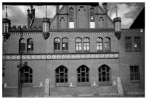
Different scale and orientation (Scale = 0.5, rotation angle = 45°)
Image size: 3000 × 2000
Remotesensing 10 00747 i007Remotesensing 10 00747 i008
Mobile phone images
Indoor environment
Uncalibrated
Different planar surfaces
Image size: 2322 × 4128
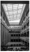
Remotesensing 10 00747 i009Remotesensing 10 00747 i010
Table 2. Numerical indicators for the first image pair.
Matching MeasuresMatching Methods
SIFTSURFORBOURS
Number of Features (F)6559664065006463
Number of Matches (M)2906370631634530
Number of Precise Matches (NPM)212615634224484
Matching Precision (MP)73.16%42.17%13.34%98.98%
Number of Accurate Matches (NAM)2586323726484125
Matching Accuracy (MA)88.99%87.34%83.71%91.06%
Percentage of Correct Matches to Feature number (PCMF)39.43%48.75%40.74%63.82%
Table 3. Numerical indicators for the second image pair.
Matching MeasuresMatching Methods
SIFTSURFORBOURS
F5872549755005217
M74818368023546
NPM112113402090
MP14.97%6.15%4.99%58.94%
NAM5254983712137
MA70.19%27.12%46.26%60.27%
PCMF8.94%9.06%6.75%40.96%
Table 4. Numerical indicators for the third image pair.
Matching MeasuresMatching Methods
SIFTSURFORBOURS
F6341639265006888
M14411772541049
NPM135349132457
MP93.75%29.65%51.97%43.57%
PCMF2.13%5.46%2.03%6.63%
Table 5. Numerical indicators for the fourth image pair.
Matching MeasuresMatching Methods
SIFTSURFORBOURS
F6559664065006201
M1337112919202670
NCM132534918222661
PCMF20.20%5.26%28.03%42.85%
MP99.10%29.65%94.84%99.63%
Table 6. Numerical indicators for the fifth image pair.
Matching MeasuresMatching Methods
SIFTSURFORBOURS
F4915489047004764
M1139173615233310
NCM973105712143024
PCMF19.80%21.62%25.83%63.48%
MP85.43%60.89%79.71%91.36%

