Article

Using Spatial Features to Reduce the Impact of Seasonality for Detecting Tropical Forest Changes from Landsat Time Series

by
Eduarda M. O. Silveira
1,*,
Inácio T. Bueno
1,
Fausto W. Acerbi-Junior
1,
José M. Mello
1,
José Roberto S. Scolforo
1 and
Michael A. Wulder
2
1
Forest Science Department, Federal University of Lavras, Lavras 37200-000, Brazil
2
Canadian Forest Service (Pacific Forestry Centre), Natural Resources Canada, 506 West Burnside Road, Victoria, BC V8Z 1M5, Canada
*
Author to whom correspondence should be addressed.
Remote Sens. 2018, 10(6), 808; https://doi.org/10.3390/rs10060808
Submission received: 19 March 2018 / Revised: 5 May 2018 / Accepted: 17 May 2018 / Published: 23 May 2018
(This article belongs to the Section Forest Remote Sensing)

Abstract

:
In forested areas that experience strong seasonality and are undergoing rapid land cover conversion (e.g., Brazilian savannas), the accuracy of remote sensing change detection is affected by seasonal changes that are erroneously classified as having changed. To improve the quality and consistency of regionally important forest change maps, we aim to separate process related change (for example, spectral variability due to phenology) from changes related to deforestations or fires. Seasonal models are typically used to account for seasonality, but fitting a model is difficult when there are insufficient data points in the time series. In this research, we utilize remotely sensed data and related spectral trends and the spatial context at the object level to evaluate the performance of geostatistical features to reduce the impact of seasonality from the NDVI (Normalized Difference Vegetation Index) of Landsat time series. The study area is the São Romão municipality, totaling 2440 km2, and is part of the Brazilian savannas biome. We first create image objects via multiresolution segmentation, basing the objects on the characteristics found in the first image (2003) of the 13-year time series. We intersected the objects with the NDVI images in order to extract semivariogram indices, the RVF (Ratio Variance—First lag) and AFM (Area First lag—First Maximum), and spectral information (average and standard deviation of NDVI values) to generate the time series from these features and to derive Spatio-Temporal Metrics (change and trend) to train a Random Forest (RF) algorithm. The NDVI spatial variability, captured by the AFM semivariogram index time series produced the best result, reaching 96.53% of the overall accuracy (OA) to separate no-change from forest change, while the greatest inter-class confusion occurred using the average of the NDVI values time series (OA = 63.72%). The spatial context approach we presented is a novel approach for the detection of forest change events that are subject to seasonality (and possible miss-classification of change) and mitigating the effects of forest phenology without the need for specific de-seasoning models.

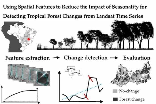
Graphical Abstract

1. Introduction

Savannas are the dominant biome in South Hemisphere, covering approximately 45% of the area of South America [1]. In Brazil, this biome consists of a mosaic of land cover types, undergoing a strong seasonality in climate, accompanied with a widespread occurrence of fires that impose environmental pressures with the most rapid land conversion in Brazil, exceeding that of the tropical forests [2]. Given the high rates of deforestation and few formally protected areas, the savanna biome is among the most endangered ecoregions on Earth [3]. Accurate mapping and monitoring of areas undergoing conversion are needed to indicate the priority areas for conservation and to inform sustainable land use management, as well as to improve the understanding of the dynamics and related impacts on carbon balance, nutrient cycling, and water resources [1]. At present, much of the effort estimating forest changes in Brazil has been focused on the tropical rainforests with less attention dedicated to the less humid seasonal regions [4]. Many different models can be used to estimate deforestation trends in tropical regions [5], however, in Brazil, most of these models were developed for the Amazon region with a few studies representing the Savannas biome [4,6]. Although human-induced disturbances are threatening these ecosystems, systematic investigations of land cover change are lacking [7].
Remotely sensed data have been widely recognized as essential data sources for comprehensive mapping and quantification of land cover changes [8,9,10,11,12,13,14]. Studies have used the NDVI (Normalized Difference Vegetation Index) time series from moderate resolution sensors (that is, MODIS) for land cover change detection benefitting from their frequent revisit time [15,16]. However, images from medium spatial resolution sources such as Landsat offer more detailed spatial information, providing insights at smaller spatial scales over a longer period of time. Initiated in 1972, Landsat is the longest running cross-calibrated globally consistent record of the Earth’s surface at a medium resolution [13]. The ability to utilize the dense time series of imagery from Landsat has been demonstrated for mapping land cover changes, such as deforestation, forest degradation, and impacts of fire [17,18,19,20,21]. Given the long time series of Landsat data at the global scale [22], the production of forest change maps is common as first steps towards estimating biomass and related CO2 emissions [23] and biodiversity loss. Based on investigations using Landsat data, the greatest total forest change due to deforestation from 2000 to 2012 of the four climate domains (tropical, subtropical, temperate, and boreal) is the tropical domain [24].
However, estimating forest change by remote sensing is not a trivial task. Satellite images can contain a combination of natural forest phenology, cloud cover, atmospheric scattering, and geometric errors [25], impairing the precision of change estimates, especially in tropical areas that exhibit strong seasonality in photosynthetic activity [12]. When images from different seasons are acquired, changes caused by phenological differences are present and can result in the mapping of a change in condition, rather than a change in land cover or land use [26]. To reduce the seasonal variations captured by remotely sensed images, techniques for de-seasoning time series have been used [27] on the assumption that seasonal patterns can be identified and removed [15,16,26,28,29]. However, this assumption may not always hold if the time series is for satellite images which are not acquired at regular intervals or have gaps due to the presence of clouds [12]. To minimize the impacts of seasonality, methods combining different satellites [30,31] and others that explore the spatial context [12] have been developed.
Previous studies have shown that pixel-based change detection can suffer from not including additional information regarding the spatial context [32]. The inclusion of spatial information can reduce the small or spurious changes [33] and also allow for the incorporation of supplemental spatial information, such as geostatistical features [34,35,36,37]. Although pixel-based approaches also generate spatial information, the neighborhood used to retrieve the information is often defined by a square window that is easy to implement. However, they are computational expensive [27], biased along their diagonals, and can straddle the boundary between two landscape features, especially when a large window size is used [38].
Here, we propose a new approach to reduce the impacts of the seasonal changes introduced by forest phenology on forest change detection using the spatial variability of Landsat NDVI time series at the object level. We hypothesize that variability measures are not affected by vegetation seasonality as the NDVI variability remains constant in the presence of seasonal changes and substantially increases in the presence of land cover changes. Thus, we investigated if the geostatistical features can be used to eliminate seasonal variations in satellite image time series and improve the change detection results. We used an object-based approach associated with a set of Spatio-Temporal Metrics by computing geostatistical features, specifically the semivariogram indices developed by Reference [35]. We also compared the change detection results to those provided by traditional spectral features (average and standard deviation of NDVI values). Implementation of this approach enables us to enrich object-based remote sensing methods using the spatial information provided by semivariograms that capture the spatial variability of images which are directly related to land cover changes, improving the change detection classification performance in highly seasonal and ecologically important environments.

2. Study Area

The study area is the São Romão municipality in the state of Minas Gerais (MG), Brazil (Figure 1a). Totaling 2440 km2, approximately 84% of this area is occupied by land cover classes comprising Brazilian savannas [39] (Figure 1b). The Brazilian savanna’s natural vegetation consists of mixtures of grasslands, shrublands, and woodlands which are found over a gradient of vegetation density, growth form, vertical structure, and biomass [40] (Figure 1c). Riparian forests are found along the rivers and streams of the study area. As vegetation progresses from grasslands to woodlands and forests, there is an increase in cover, height, density, and the basal area of the trees present [41]. Our analysis focused on the main vegetation types found in the study area (Table 1): open grassland, open grassland with sparse shrubs, mixed grassland, shrublands, trees up to seven meters, and riparian vegetation (palm swamps and semideciduous forests) [42,43]. The climate is typically tropical (Aw) with rains concentrated in the October–May period, which characterizes the high seasonality in the region [44].

3. Methodology

We introduce a method for object-based change detection using geostatistical features to derive Spatio-Temporal Metrics from the time series, eliminating the effect of forest phenology. The method is divided into three main steps (Figure 2).
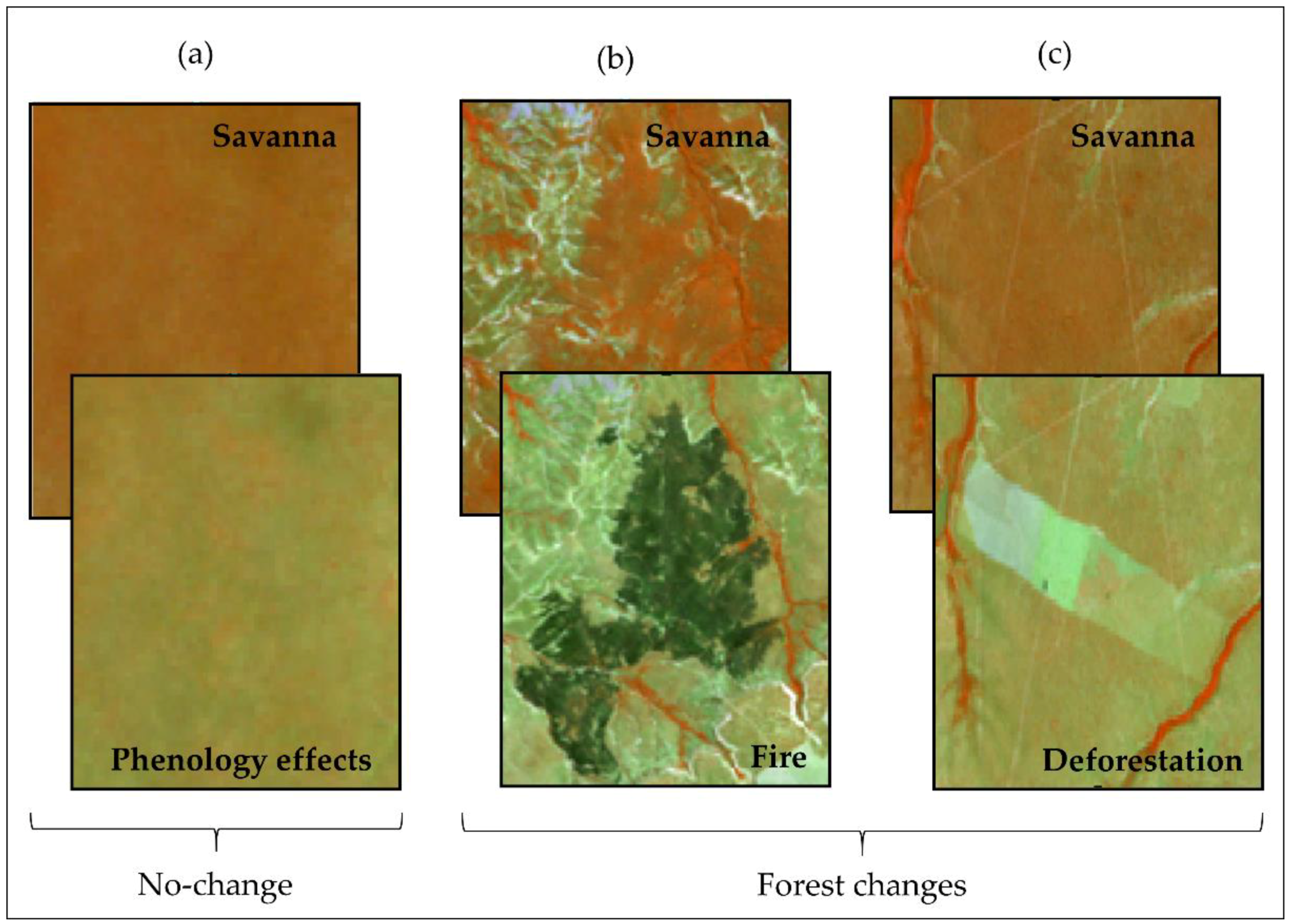
We chose as the change target the Brazilian savannas land-cover classes and the following change agents (Figure 3):
  • No-change: seasonal changes due to phenological effects (natural events)
  • Forest change: land cover changes such as deforestation (human-induced) and fires (both natural events and human induces)

3.1. Satellite Data and Processing

We downloaded all available cloud-free Landsat TM (Thematic Mapper) and OLI (Operational Land Imager) images between 2003 to 2016 (total of 66 images) from the free and open access USGS Earth Resources Observation and Science (EROS) Center archive (Table 2). The data as downloaded is already processed to surface reflectance using the Landsat Ecosystem Disturbance Adaptive Processing System (LEDAPS) and L8SR algorithm, respectively. Clouds and cloud shadows have been masked with the CFmask function [45].
We used the NDVI vegetation index [46] for further analysis. The advantages of using indices rather than the original spectral band observations include minimizing the soil and other background effects, reducing data dimensionality, providing a degree of standardization for comparison, and enhancing the vegetation signal [47].

3.2. Object-Based Image Analysis

Image segmentation is the division of the satellite image into groups of pixels spatially continuous and spectrally homogeneous, minimizing the within-object variability compared to the between-object variability [48]. We used the multiresolution segmentation algorithm [49] implemented in the eCognition software. eCognition is a powerful development environment for object-based image analysis designed to produce homogeneous image objects based on spatial and spectral homogeneity criteria. The eCognition technology examines image pixels not in isolation, but in the spectral and spatial contexts. It builds up a given segmentation iteratively, recognizing groups of pixels as objects, using color, shape, texture, shape, and the size of objects, as well as their context and relationships [50].
Three different choices are typically considered when defining the analysis unit (image objects) for multitemporal object-based image analysis [51]: (i) image-object overlay: image-objects are generated by segmenting one of the images in the time series. A comparison against other images is then made by simple overlay; (ii) image-object comparison: image-objects are generated by segmenting each image in the time series independently; and (iii) multitemporal image-object: image-objects are generated by segmenting the entire time series together. Our study focused on the image-object overlay approach, as expected to capture the intra-object heterogeneity well.
Three key segmentation parameters (shape, compactness, and scale) control the size, shape, and spectral variation of segmented image objects [52]. We set the shape and compactness parameter to 0.1 and 0.5, respectively. The scale parameter controls the size of the image objects and sets a homogeneity threshold that determines the number of neighboring pixels that can be merged together to form an image object [53]. The scale of segmentation directly influences the size of the objects connected to the semivariogram predefined criteria (lag distance) and the minimum number of pixels inside each object necessary to generate the semivariogram makes this segmentation parameter crucial at this point. Based upon starting values found in the literature [48], we then used a “trial-and-error” approach [54] to find the appropriate scale parameter [55] that was set to 150 [37]. The image segmentation outputs were assessed based on a visual assessment of segmentation suitability. The segmentation parameters were also defined to generate sufficiently small objects to not be spatially or spectrally confused, yet large enough to allow for calculation of the semivariogram and related geostatistical features.

3.3. Geostatistical and Spectral Features

We used two semivariogram indices [35] as geostatistical features (Table 3). Inside each object, we extracted the NDVI values to generate the experimental semivariogram and calculate the semivariogram indices. The experimental semivariogram is defined as half of the average squared difference between values separated by a given lag, where this lag is a vector in both, distance, and directions [56]. It was estimated using Equation (1):
γ ( h ) = 1 2 N ( h ) i = 1 N ( h ) [ Z ( x ) - Z ( x + h ) ] 2 ,
where γ (h) is the estimator of the semivariance for each distance h, N(h) is the number of pairs of points separated by the distance h, Z(x) is the value of the regionalized variable in the point x and Z(x + h) is the value of the point (x + h).
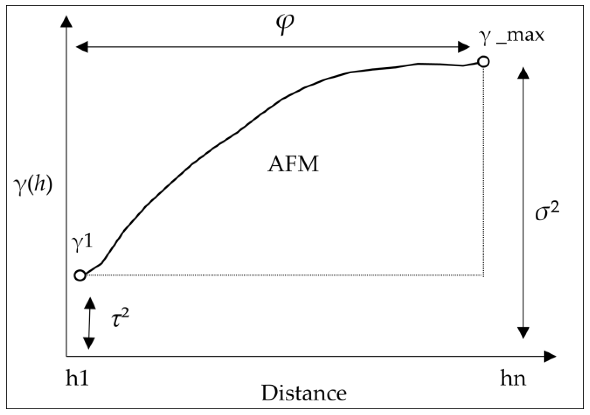
The graphic for spatial variance versus distance h represents the semivariogram, which allows obtaining the estimate of the variance value for different combinations of pairs of points. The semivariance functions are characterized by three parameters: sill (σ2), range (ϕ), and nugget effect (τ2). The sill parameter is the plateau reached by semivariance values and shows the quantity of variation explained by the spatial structure of the data. The range parameter is the distance where the semivariogram reaches the sill, showing the distance until where the data are correlated. The nugget effect is the combination of sampling errors and variations that happen in scales smaller than the distance between the sampled points [57].
When the semivariogram is calculated at the object level, an important factor for consideration is the lag distance. It should not be larger than the spatial extent of the object; on the other hand, an exceedingly small distance fails to provide a complete description of textural features. We attempted to find an optimal lag distance to ensure that sill values would provide a concise description of data variability. We fixed the number of lags as 20 pixels and the lag size equivalent to image spatial resolution (30 m), resulting in a lag distance of 600 m [37,58].
Using FETEX 2.0 [59], we calculated the semivariogram indices that describe the shape of the experimental semivariograms and, therefore, the properties that characterize the spatial patterns of each image object. In addition, fitting a model is unnecessary, which reduces both processing time and possible errors from choosing a sub-optimal model. FETEX 2.0 is a software application enabling automatic descriptive feature extraction from image-objects. The input data include a multispectral digital image or single band, such as NDVI, and a vector file in shapefile format containing the boundaries of the objects. The output file is a table containing a vector of features for every object processed. This table of numeric values describing the objects from different points of view can be then used as the input data to other classification software.
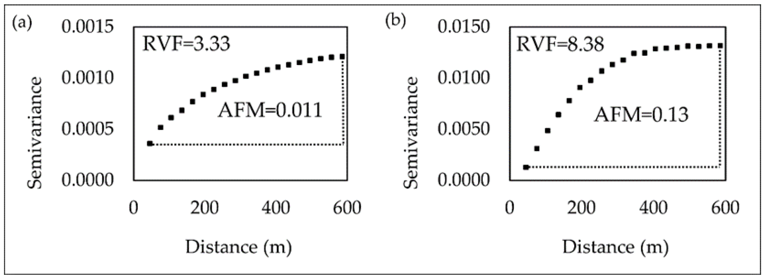
RVF is the ratio between the values of the total variance γ max _ 1 and the semivariance at first lag ( γ 1 ) . Since the semivariogram tends to reach the sill near the total variance, this parameter is an indicator of the relationship between the spatial correlation at long and short distances. Its value increases when the high variability at long distances and low variability at short distances occurs. This feature also presents high values for images with large primitives or periodic patterns [35]. AFM is the area between the semivariogram value in the first lag and the semivariogram. This parameter provides information about the semivariogram curvature and is also related to the variability of the data (Figure 4).
To verify the potential of the semivariogram indices, we also used spectral features for comparative purpose. We extracted the average and standard deviation (STDV) of the NDVI values inside the objects.

3.4. Time Series

To generate the time series, we included objects intersecting savanna land cover classes in the Landsat TM image acquired in July 2003 (first image of time series) and excluded classes as water, pasture, bare soil, crops, and urban areas. We used a land cover map [39] and subsequently, we performed a post-classification editing of the imagery carried out by a skilled human interpreter using the false color composite of the corresponding image (see Figure 1b). We overlapped the savanna objects with the remaining NDVI images in order to extract the geostatistical (RVF and AFM indices) and spectral features (average and STDV) and then generated the time series (Figure 5).

3.5. Spatio-Temporal Metrics (STM)

We transformed the geostatistical and spectral features time series into two summary variables: Change and Trend, adapted from Reference [16]. As described by Reference [51], change is the maximum interannual absolute difference in the time series data within the period 2003–2016 (Equation (2)). The trend is the slope of linear regression applied to the full time series (Equation (3)).
Change =   Max   ( Feature t - Feature t + 1 ) ,
Trend = n ( t = 1 t = n t   Feature t ) - ( t = 1 t = n Feature t )   ( t = 1 t = n t ) n ( t = 1 t = n t 2 ) - ( t = 1 t = n t ) 2 ,
The Change variable contains information on the greatest positive or negative change between consecutive data. A high value indicates that a high magnitude change occurred or there is an influence of seasonal variation of the feature response. The Trend variable indicates the overall (increasing, decreasing, or none) trend in the amount of green vegetation across the entire period [16].

3.6. Random Forest Algorithm

We used the Spatio-Temporal Metrics (STM) derived from geostatistical and spectral features to train the Random Forest (RF) algorithm [60] (Figure 6). These metrics were obtained from the time series of four features (RVF, AFM, Average, and STDV) extracted from NDVI values inside objects, forming four groups of input files as described in Table 4.
RF is an ensemble method which generates a set of individually trained decision trees and combines their results. RF is a robust non-parametric classifier and can accommodate many predictor variables [19]. The advantages of RF include effectiveness in prediction, efficient implementation on large datasets [60], and insensitivity to noise in the training data [61]. We used the Random Forest package [60] available as an R package [62].
Two parameters need to be set in order to produce the random forest trees: the number of decision trees to be generated (Ntree) and the number of variables to be selected and tested for the best split when growing the trees (Mtry) [63]. The Gini criterion is used to select the split with the lowest impurity (highest homogeneity) at each node. For each tree, the predicted class for each observation is obtained and the class with the maximum number of votes among the trees is the predicted class of an observation [64].
The Ntree required to maintain a given level of accuracy has been assessed by several authors, and the minimum number of trees for optimal classification appears to be between 100 [65] and 300 [66], with the majority of studies setting the Ntree value to 500 because the errors stabilize before this number of classification trees is achieved [65]. Five hundred trees were grown for each classification and the number of features (Mtry = 1) was left at its default values.

3.7. Change Detection Evaluation

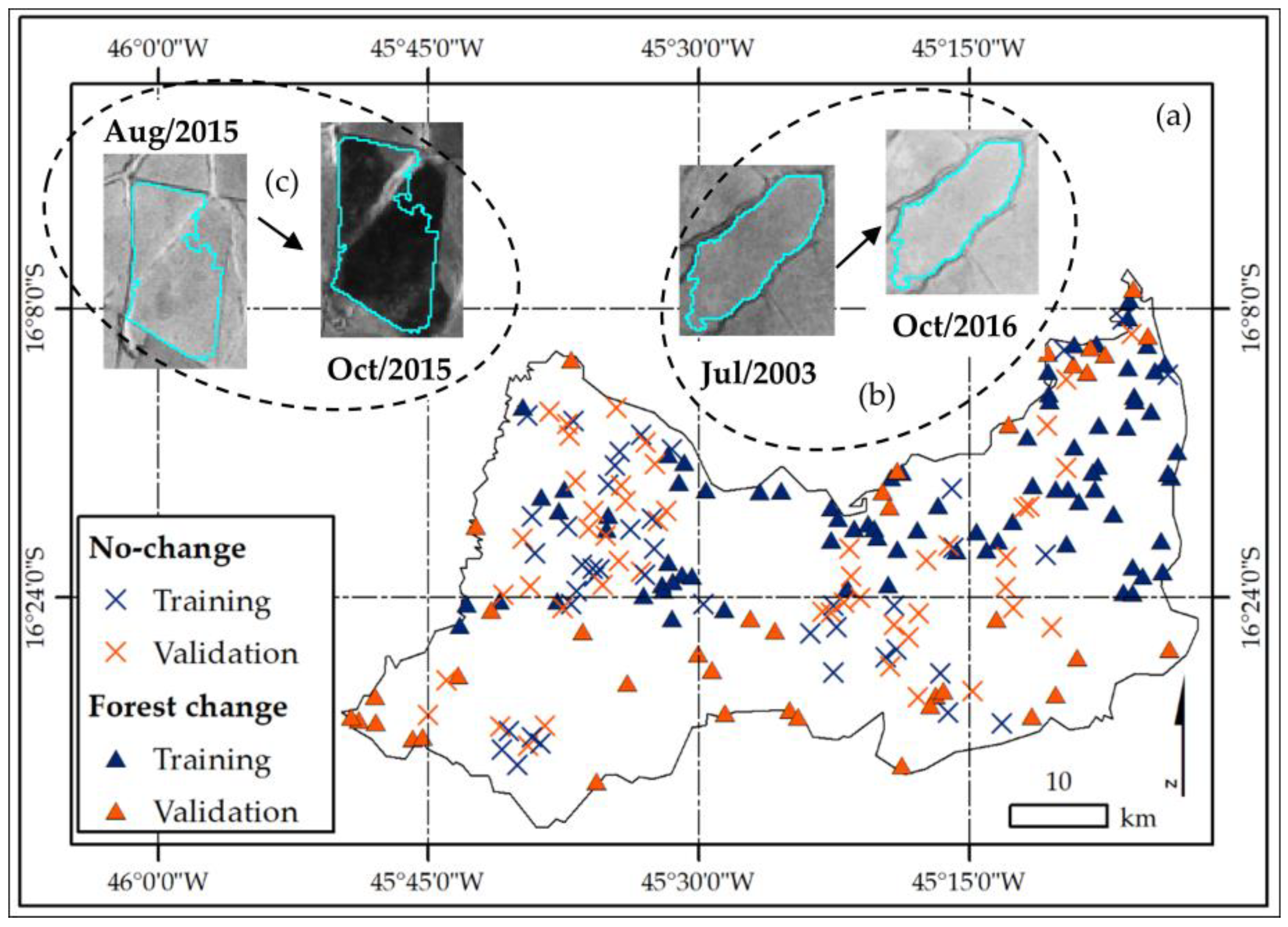
Evaluation of change detection outcomes is communicated using a confusion matrix [67] and its accuracy measures: overall accuracy (OA), producer accuracy (PA), user accuracy (UA), and the kappa coefficient (k). A dataset of 1000 objects well-distributed over the study area, with 500 samples per class (Table 5), was assigned based on visual interpretation (Figure 7a). The objects of no-change were those where no changes were found during the entire analyzed period 2003–2016 (Figure 7b). Otherwise, regardless of the date when changes have occurred, the objects undergoing a deforestation or fires were selected and identified as forest change (Figure 7c). Seventy percent of the samples were randomly chosen as training samples, while the rest were used as validation samples. We used the class-stratified random sampling design that provides the option to increase the sample size in classes that occupy a small proportion of area and is one of the easier designs to implement [68].
The evaluated performances were compared among the four input features (average, standard deviation, RVF, and AFM) through the confusion matrix measures. We also generated a validation map to identify the savannas land cover changes (deforestation and fires) by visual interpretation to spatialize the areas classified as correct and incorrect. We used as reference data, a land cover map [39] which described qualitative and quantitative information of savannas vegetation type in the state of Minas Gerais, Brazil.

4. Results

4.1. Semivariogram Analysis

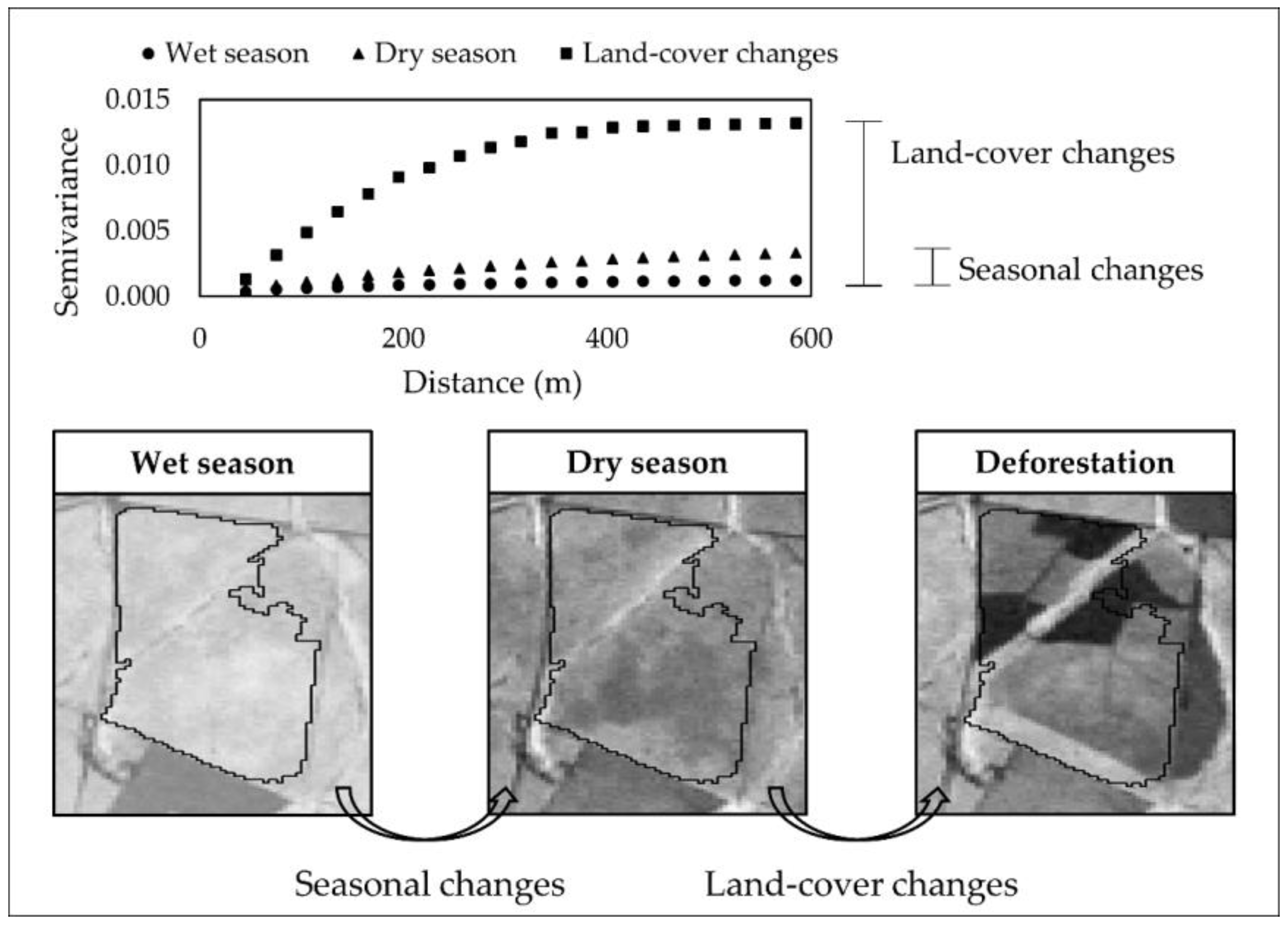
We analyzed the temporal-spatial variability of NDVI data comparing the semivariogram shape and indices. The semivariograms reached the sill (σ2) within the calculated distance (600 m), indicating that their spatial extents were sufficiently large to encompass the entire spatial variability. From no-change transitions (landscape vegetation cover that had the same land cover classes in both times, encompassing seasonal variations due to vegetation phenology), NDVI semivariograms had similar behaviors, presenting sill values around 0.0010 (Figure 8a,b). In the presence of changes (that is, fires), NDVI semivariograms considerably increased, reaching sill values around 0.0060 (Figure 8c). Note how the shape and sill parameter of no-change areas remained constant, but changed markedly in areas with human activities (Figure 8d).
These results indicate a very clear trend whereby the overall variability and shape, the semivariogram increased when land cover changes occurred, and were similar when the area had not undergone any land cover change. These results demonstrate that the semivariograms derived from NDVI images, is not affected by phenological changes (remain constant), while also demonstrating the potential of detecting land cover changes (notably increase) due to the mosaic of types of landscape with low NDVI and high NDVI, increases the NDVI spatial variability.

4.2. Change Detection

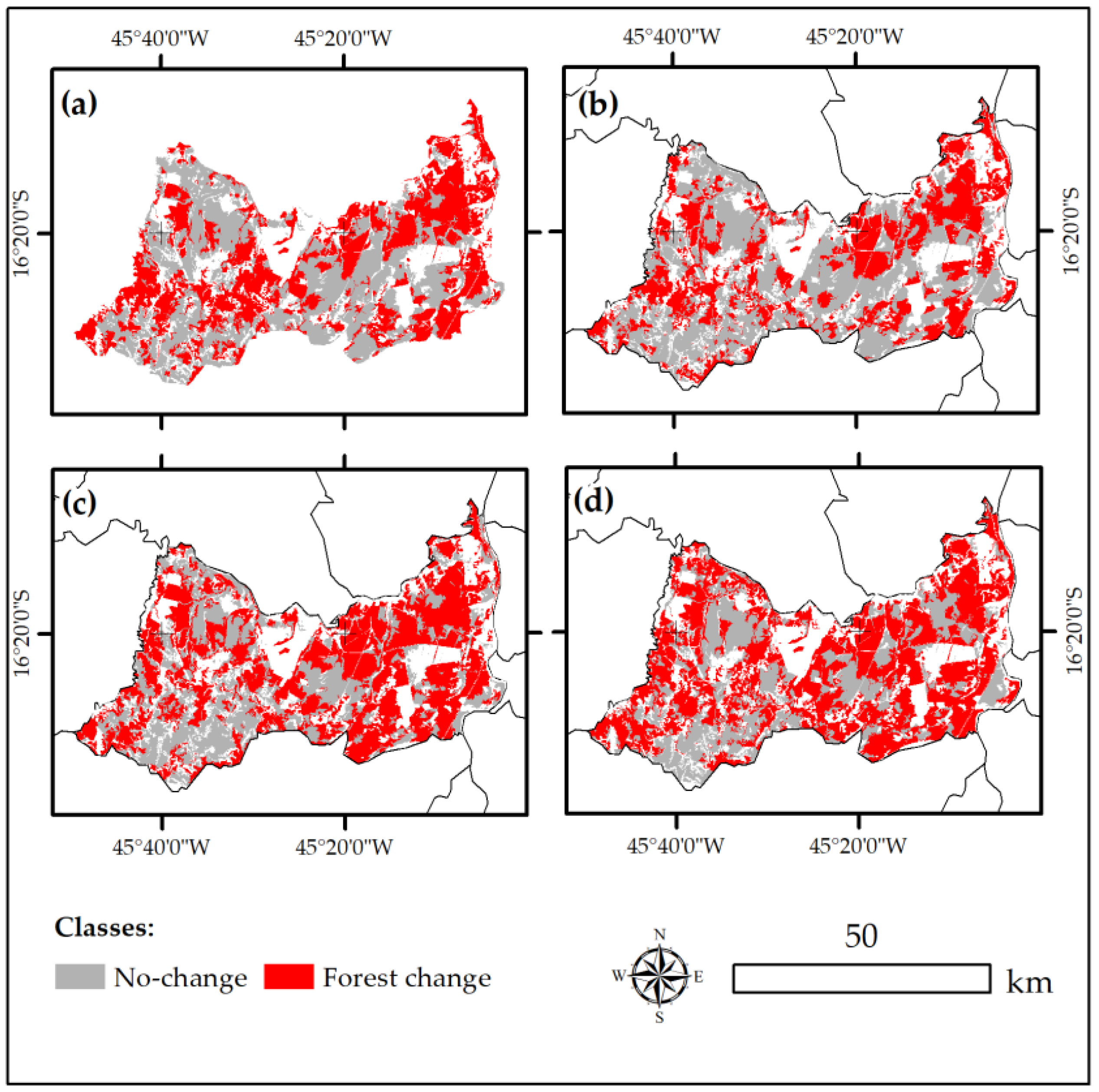
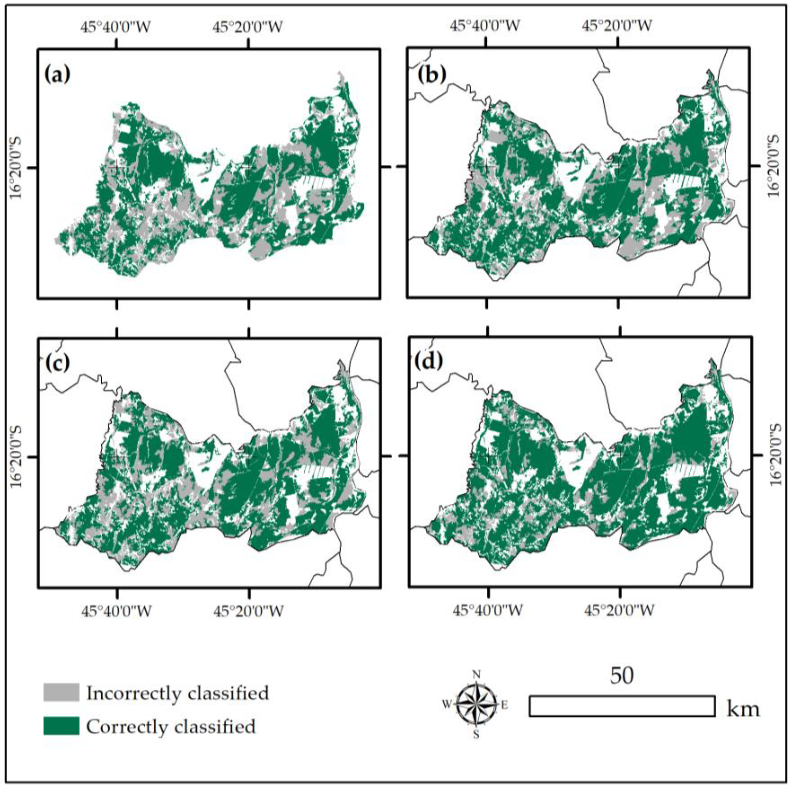
We used the Change and Trend Spatio-Temporal Metrics derived from geostatistical and spectral features time series as input data to train the random forest (RF) algorithm. The classification results (Figure 9) achieved overall accuracies from 63.7% to 96.5%, with user’s accuracies ranging from 61.5% to 98.2% and producer’s accuracies from 58.9% to 97.7% (Table 6). The AFM index provided the best results, reaching 96.5% of the overall accuracy and a 0.9 kappa index. The standard deviation also produced good results, with a kappa index reaching 0.8. The greatest inter-class confusion occurred using the average of the NDVI values and RVF index, revealing low values of overall, producer and user accuracies and kappa index.
As a result, the feature average and the semivariogram index RVF were not able to accurately capture the differences between forest change and seasonal changes. These features are sensitive to phenological variations, resulting in the false detection of LULC changes, overestimating the areas undergoing fire or deforestation (Figure 10a,c). The standard deviation spectral feature presented good accuracy measures (overall accuracy reaching 88.3%), however, the map generated was not more accurate (Figure 10b). The AFM semivariogram index provided the best result. This index is directly influenced by the sill (σ2) semivariogram parameter (overall variability), which is sensitive to land cover changes and is not affected by changes caused by vegetation seasonality, providing good classification results (Figure 10d).

5. Discussion

5.1. NDVI Spatial Variability

To capture the NDVI variability inside the objects we used the semivariogram, that is a graphical representation of the spatial variability in a given dataset [69], provided by the sill (σ2), range (ϕ), and nugget effect (τ2) parameters. The semivariogram presents the ability to depict landscape spatial heterogeneity [70]. The differences of NDVI spatial variability between landscapes are mainly explained by the type of landscape, where the image spatial variability (sill-σ2) increases considerably from homogeneous to heterogeneous areas.
The semivariogram shape and metrics generated from NDVI values, derived from Landsat TM images are useful in detecting deforestation in areas covered by savanna vegetation [62]. In deforested areas, the landscape change caused spatial variations that were quantified by the semivariogram metrics of range, sill, and shape. The range and sill were the two most important and complementary metrics. Both metrics increased their values after deforestation and remain similar if the land cover had not been changed.
Here, instead of using the semivariogram parameters to quantify the NDVI spatial variability we used the RVF and AFM semivariogram indices as they synthesize the most relevant information about the shape of the semivariogram. In addition, fitting a model is unnecessary, which shortens the processing time and reduces the errors generated by choosing a sub-optimal model [35]. From the wet to dry season, the NDVI spatial variability is almost constant and in the presence of land cover changes, such as deforestation and fires, the NDVI variability highly increased (Figure 11). The preserved savannas land cover classes (both in wet and dry seasons) have low NDVI variability compared to disturbed savannas land cover classes. These high values are explained by the presence of high and low NDVI values in the same object, as land cover changes exceed seasonal variability.
The total variance of NDVI values increases considerably from homogeneous to heterogeneous landscapes. In homogeneous objects as preserved savannas, the NDVI semivariance among the pixels is low, thus, the RVF index is also low because the ymax (~0.0013) is almost similar with the semivariance in the first lag (~0.0005). The AFM is also small (0.011) (Figure 12a). In heterogeneous objects, such as savannas undergoing a deforestation or fires, the RVF and AFM indices considerably increase, ranging from 3.33 to 8.38 and 0.011 to 0.13, respectively (Figure 12b).
Similar patterns were found by Reference [37] exploring and evaluating the performance of semivariogram indices derived from NDVI images in an object-based approach to detect land cover changes. The image’s spatial variability changed considerably from native vegetation (pre-disaster image) to flooded areas (post-disaster image). The flooded areas had a low overall variability compared to native vegetation, making the detection of change using the semivariogram possible.

5.2. Seasonal Effects on Change Detection

We hypothesized that the semivariogram indices (RVF and AFM) are not affected by vegetation seasonality due to the NDVI variability remaining constant in the presence of seasonal changes and substantially increases in the presence of land cover changes, such as deforestation and fires (both natural events and human-induced).
Remote sensing of vegetation has an implied link to vegetation phenology. Phenology is an environmental process that operates independently of land cover or land use change. The ability to use remote sensing images to detect changes in seasonal areas relies on the capacity to remove the effects of seasonal variations, while still identifying changes caused by deforestation, urbanization, floods, and fires. To avoid the classification of seasonal effects as land cover change, time series have been used to derive the seasonal patterns when mapping deforestation. For instance, Verbesselt et.al developed a powerful change detection approach for time series, using 16-day MODIS NDVI images, involving the detection and characterization of Breaks For Additive Seasonal and Trend (BFAST) that integrates the iterative decomposition of time series into trend, seasonal, and noise components with methods for detecting changes, without the need to select a reference period, set a threshold, or define a change trajectory [15].
Rather than using the BFAST seasonal model to account for seasonality in the image time series, Hamunyela et.al researches used the spatial context in a pixel-based approach using Landsat data assessing how the size of spatial window influences the deforestation detection and related computational time [12]. They demonstrated that, in dry tropical forests, deforestation events are detected much earlier when the spatial context approach is used than when a seasonal model is used. Smaller spatial windows achieved higher overall spatial accuracy than larger windows and increasing the size of the spatial window resulted in a linear increase in the computational time per pixel.
The window size is an important aspect of the spatial context method since it influences the resultant spatial information due to the amount of variance included [71,72]. The spatial moving window needs to be sufficiently larger than the size of the deforestation event to avoid smoothing out the disturbance impact from the time series, and also for it to capture local variations [12].
Here, we used the spatial context (semivariogram indices) in an object-based approach, without the need of use of the spatial window, basing the objects on the characteristics found in the first image of the time series. The time series of the AFM semivariogram index provided the best separability (global accuracy = 96.53%) between objects with seasonal changes and objects undergoing a forest change. Similar results were found by Reference [73], assessing the potential of individual geostatistical features derived from bitemporal NDVI images to accurately detect land cover changes. They demonstrated that the accuracies of the sill parameter and AFM semivariogram indices were higher than those of the other indices, which were not affected by vegetation seasonality because they represent the information provided by the entire semivariogram rather than specific parts of it.

5.3. Method Limitations

Despite the good performance of the proposed method, in this section, two limitations to the approach used in this study are elaborated upon, including the quantification of areas changed and the timing of forest changes:
(1)
Forest change quantification: The method can identify the objects undergoing land cover changes without being impacted by seasonal variations; however, it is not possible to accurately calculate the changed area. Due to use of an object-based approach, some changes do not cover the entire object because the forest change class comprised both small changes reaching up to 20% of the objects and large changes ranging from 50% to 100% of the object area. This limitation is related to the initial image segmentation performed on the first image of the time series (image object overlay) rather than segmenting the entire time series (multitemporal image object). We used this technique because it provides a more meaningful framework for spatial measures [51], capable of capturing the intra-object heterogeneity [74]. Further research into how the proportion of pixels changed inside the objects (real area of forest change) affect the resultant accuracies remain outstanding.
(2)
Timing of changes: The method allows for the discrimination between forest change and no-change classes, however, it is not possible to indicate when exactly the forest changes have occurred. Although the timing of the change is an important feature of forest monitoring, we did not attempt to model the time of the change, as our main focus is not hinged on the capacity to date forest changes, rather we focus on the advantages of using variability measures as input data to train the RF algorithm.

6. Conclusions

We have developed a method to mitigate the presence of phenological effects from time series using NDVI trends to detect changes over a savannah forest ecosystem. The approach combining spatial and spectral information and allowed for the detection of changes without being impacted by seasonal variations. We demonstrated that NDVI spatial variability, captured by AFM semivariogram index, is not affected by vegetation seasonality and, therefore, can produce time series that accurately differentiate forest changes from seasonal changes, resulting in fewer classification errors. Our proposed method is simple and accurate, efficiently detecting changes while eliminating the effects of phenology.
The spatial context approach we presented in this paper is a novel and useful object-based remote sensing method for the detection of forest change events using Landsat NDVI data in areas where forests exhibit strong seasonality (that is, in Brazilian seasonal biomes). Our results demonstrate that the semivariograms derived from NDVI images are not affected by phenological changes (remain largely constant). The spectral values may differ over time within a given year, but absent actual change (for example, fire or deforestation), the amount and nature of the variability present at the object level remains similar. This method addresses the challenge of accurately detecting deforestation and fires without erroneously labeling seasonal phenological differences as changes without the need to use de-seasoning models.

Author Contributions

These authors equally contributed to this work.

Funding

This research received no external funding.

Acknowledgments

The authors are grateful to the Coordenação de Aperfeiçoamento de Pessoal de Nível Superior (CAPES) and the Department of Forest Science of the Federal University of Lavras (UFLA) for supporting this work.

Conflicts of Interest

The authors declare no conflicts of interest.

References

  1. Sano, E.E.; Rosa, R.; Brito, J.L.S.; Ferreira, L.G. Land cover mapping of the tropical savanna region in Brazil. Environ. Monit. Assess. 2010, 166, 113–124. [Google Scholar] [CrossRef] [PubMed]
  2. Ferreira, L.G.; Yoshioka, H.; Huete, A.; Sano, E.E. Seasonal landscape and spectral vegetation index dynamics in the Brazilian Cerrado: An analysis within the Large-Scale Biosphere–Atmosphere Experiment in Amazônia (LBA). Remote Sens. Environ. 2003, 87, 534–550. [Google Scholar] [CrossRef]
  3. Hoekstra, J.M.; Boucher, T.M.; Ricketts, T.H.; Roberts, C. Confronting a biome crisis: Global disparities of habitat loss and protection. Ecol. Lett. 2004, 8, 23–29. [Google Scholar] [CrossRef]
  4. Beuchle, R.; Grecchi, R.C.; Shimabukuro, Y.E.; Seliger, R.; Eva, H.D.; Sano, E.; Achard, F. Land cover changes in the Brazilian Cerrado and Caatinga biomes from 1990 to 2010 based on a systematic remote sensing sampling approach. Appl. Geogr. 2015, 58, 116–127. [Google Scholar] [CrossRef]
  5. Verburg, P.H.; Schot, P.P.; Dijst, M.J.; Veldkamp, A. Land use change modelling: Current practice and research priorities. GeoJournal 2004, 61, 309–324. [Google Scholar] [CrossRef]
  6. Espírito-Santo, M.M.; Leite, M.E.; Silva, J.O.; Barbosa, R.S.; Rocha, A.M.; Anaya, F.C.; Dupin, M.G.V. Understanding patterns of land-cover change in the Brazilian Cerrado from 2000 to 2015. Philos. Trans. R. Soc. B Biol. Sci. 2016, 371, 20150435. [Google Scholar] [CrossRef] [PubMed]
  7. Dupin, M.G.V.; Espírito-Santo, M.M.; Leite, M.E.; Silva, J.O.; Rocha, A.M.; Barbosa, R.S.; Anaya, F.C. Land use policies and deforestation in Brazilian tropical dry forests between 2000 and 2015. Environ. Res. Lett. 2018, 13, 35008. [Google Scholar] [CrossRef]
  8. Yuan, F.; Sawaya, K.E.; Loeffelholz, B.C.; Bauer, M.E. Land cover classification and change analysis of the Twin Cities (Minnesota) Metropolitan Area by multitemporal Landsat remote sensing. Remote Sens. Environ. 2005, 98, 317–328. [Google Scholar] [CrossRef]
  9. De Sy, V.; Herold, M.; Achard, F.; Asner, G.P.; Held, A.; Kellndorfer, J.; Verbesselt, J. Synergies of multiple remote sensing data sources for REDD+ monitoring. Curr. Opin. Environ. Sustain. 2012, 4, 696–706. [Google Scholar] [CrossRef]
  10. Grecchi, R.C.; Gwyn, Q.H.J.; Bénié, G.B.; Formaggio, A.R.; Fahl, F.C. Land use and land cover changes in the Brazilian Cerrado: A multidisciplinary approach to assess the impacts of agricultural expansion. Appl. Geogr. 2014, 55, 300–312. [Google Scholar] [CrossRef]
  11. DeVries, B.; Verbesselt, J.; Kooistra, L.; Herold, M. Robust monitoring of small-scale forest disturbances in a tropical montane forest using Landsat time series. Remote Sens. Environ. 2015, 161, 107–121. [Google Scholar] [CrossRef]
  12. Hamunyela, E.; Verbesselt, J.; Herold, M. Using spatial context to improve early detection of deforestation from Landsat time series. Remote Sens. Environ. 2016, 172, 126–138. [Google Scholar] [CrossRef]
  13. Schultz, M.; Clevers, J.G.P.W.; Carter, S.; Verbesselt, J.; Avitabile, V.; Quang, H.V.; Herold, M. Performance of vegetation indices from Landsat time series in deforestation monitoring. Int. J. Appl. Earth Obs. Geoinf. 2016, 52, 318–327. [Google Scholar] [CrossRef]
  14. Hamunyela, E.; Reiche, J.; Verbesselt, J.; Herold, M. Using Space-Time Features to Improve Detection of Forest Disturbances from Landsat Time Series. Remote Sens. 2017, 9, 515. [Google Scholar] [CrossRef]
  15. Verbesselt, J.; Hyndman, R.; Newnham, G.; Culvenor, D. Detecting trend and seasonal changes in satellite image time series. Remote Sens. Environ. 2010, 114, 106–115. [Google Scholar] [CrossRef]
  16. Hird, J.N.; Castilla, G.; McDermid, G.J.; Bueno, I.T. A Simple Transformation for Visualizing Non-seasonal Landscape Change From Dense Time Series of Satellite Data. IEEE J. Sel. Top. Appl. Earth Obs. Remote Sens. 2016, 9, 3372–3383. [Google Scholar] [CrossRef]
  17. Wulder, M.A.; Masek, J.G.; Cohen, W.B.; Loveland, T.R.; Woodcock, C.E. Opening the archive: How free data has enabled the science and monitoring promise of Landsat. Remote Sens. Environ. 2012, 122, 2–10. [Google Scholar] [CrossRef]
  18. Zhu, Z.; Woodcock, C.E.; Olofsson, P. Continuous monitoring of forest disturbance using all available Landsat imagery. Remote Sens. Environ. 2012, 122, 75–91. [Google Scholar] [CrossRef]
  19. DeVries, B.; Pratihast, A.K.; Verbesselt, J.; Kooistra, L.; Herold, M. Characterizing Forest Change Using Community-Based Monitoring Data and Landsat Time Series. PLoS ONE 2016, 11, e0147121. [Google Scholar] [CrossRef] [PubMed]
  20. Bartels, S.F.; Chen, H.Y.H.; Wulder, M.A.; White, J.C. Trends in post-disturbance recovery rates of Canada’s forests following wildfire and harvest. For. Ecol. Manag. 2016, 361, 194–207. [Google Scholar] [CrossRef]
  21. White, J.C.; Wulder, M.A.; Hermosilla, T.; Coops, N.C.; Hobart, G.W. A nationwide annual characterization of 25 years of forest disturbance and recovery for Canada using Landsat time series. Remote Sens. Environ. 2017, 194, 303–321. [Google Scholar] [CrossRef]
  22. Hansen, M.C.; Loveland, T.R. A review of large area monitoring of land cover change using Landsat data. Remote Sens. Environ. 2012, 122, 66–74. [Google Scholar] [CrossRef]
  23. Houghton, R.A.; Byers, B.; Nassikas, A.A. A role for tropical forests in stabilizing atmospheric CO2. Nat. Clim. Chang. 2015, 5, 1022–1023. [Google Scholar] [CrossRef]
  24. Hansen, M.C.; Potapov, P.V.; Moore, R.; Hancher, M.; Turubanova, S.A.; Tyukavina, A.; Thau, D.; Stehman, S.V.; Goetz, S.J.; Loveland, T.R.; et al. High-Resolution Global Maps of 21st-Century Forest Cover Change. Science 2013, 342, 850–853. [Google Scholar] [CrossRef] [PubMed]
  25. Roy, D.P.; Borak, J.S.; Devadiga, S.; Wolfe, R.E.; Zheng, M.; Descloitres, J. The MODIS Land product quality assessment approach. Remote Sens. Environ. 2002, 83, 62–76. [Google Scholar] [CrossRef]
  26. Lu, M.; Chen, J.; Tang, H.; Rao, Y.; Yang, P.; Wu, W. Land cover change detection by integrating object-based data blending model of Landsat and MODIS. Remote Sens. Environ. 2016, 184, 374–386. [Google Scholar] [CrossRef]
  27. Zhu, Z. Change detection using landsat time series: A review of frequencies, preprocessing, algorithms, and applications. ISPRS J. Photogramm. Remote Sens. 2017, 130, 370–384. [Google Scholar] [CrossRef]
  28. Verbesselt, J.; Hyndman, R.; Zeileis, A.; Culvenor, D. Phenological change detection while accounting for abrupt and gradual trends in satellite image time series. Remote Sens. Environ. 2010, 114, 2970–2980. [Google Scholar] [CrossRef]
  29. Verbesselt, J.; Zeileis, A.; Herold, M. Near real-time disturbance detection using satellite image time series. Remote Sens. Environ. 2012, 123, 98–108. [Google Scholar] [CrossRef]
  30. Dutrieux, L.P.; Verbesselt, J.; Kooistra, L.; Herold, M. Monitoring forest cover loss using multiple data streams, a case study of a tropical dry forest in Bolivia. ISPRS J. Photogramm. Remote Sens. 2015, 107, 112–125. [Google Scholar] [CrossRef]
  31. Zhang, J. Multi-source remote sensing data fusion: Status and trends. Int. J. Image Data Fusion 2010, 1, 5–24. [Google Scholar] [CrossRef]
  32. Chen, G.; Hay, G.J.; de Carvalho, L.M.T.; Wulder, M.A. Object-based change detection. Int. J. Remote Sens. 2012, 33, 4434–4457. [Google Scholar] [CrossRef]
  33. Hussain, M.; Chen, D.; Cheng, A.; Wei, H.; Stanley, D. Change detection from remotely sensed images: From pixel-based to object-based approaches. ISPRS J. Photogramm. Remote Sens. 2013, 80, 91–106. [Google Scholar] [CrossRef]
  34. Sertel, E.; Kaya, S.; Curran, P.J. Use of Semivariograms to Identify Earthquake Damage in an Urban Area. IEEE Trans. Geosci. Remote Sens. 2007, 45, 1590–1594. [Google Scholar] [CrossRef]
  35. Balaguer, A.; Ruiz, L.A.; Hermosilla, T.; Recio, J.A. Definition of a comprehensive set of texture semivariogram features and their evaluation for object-oriented image classification. Comput. Geosci. 2010, 36, 231–240. [Google Scholar] [CrossRef]
  36. Gil-Yepes, J.L.; Ruiz, L.A.; Recio, J.A.; Balaguer, A.; Hermosilla, T. Description and validation of a new set of object-based temporal geostatistical features for land-use/land-cover change detection. ISPRS J. Photogramm. Remote Sens. 2016, 121, 77–91. [Google Scholar] [CrossRef]
  37. Silveira, E.M.d.O.; Acerbi Júnior, F.W.; Mello, J.M.D.; Bueno, I.T. Object-based change detection using semivariogram indices derived from NDVI images: The environmental disaster in Mariana, Brazil. Ciência e Agrotecnologia 2017, 41, 554–564. [Google Scholar] [CrossRef]
  38. Laliberte, A.S.; Rango, A. Texture and Scale in Object-Based Analysis of Subdecimeter Resolution Unmanned Aerial Vehicle (UAV) Imagery. IEEE Trans. Geosci. Remote Sens. 2009, 47, 761–770. [Google Scholar] [CrossRef]
  39. Carvalho, L.M.T.; Scolforo, J.R.S.; Oliveira, A.D.; Mello, J.M.; de Oliveira, L.T.; Acerbi Júnior, F.W.; Cavalcanti, H.C.; Filho, R.V. “Procedimentos de mapeamento”. In Mapeamento e Inventário. da Flora e dos Reflorestamentos de Minas Gerais; UFLA: Lavras, Brazil, 2006; pp. 37–57. [Google Scholar]
  40. Schwieder, M.; Leitão, P.J.; Bustamante, M.M.d.C.; Ferreira, L.G.; Rabe, A.; Hostert, P. Mapping Brazilian savanna vegetation gradients with Landsat time series. Int. J. Appl. Earth Obs. Geoinf. 2016, 52, 361–370. [Google Scholar] [CrossRef]
  41. Batalha, M.A.; Mantovani, W.; Mesquita Júnior, H.N. Vegetation structure in cerrado physiognomies in South-eastern Brazil. Braz. J. Biol. 2001, 61, 475–483. [Google Scholar] [CrossRef] [PubMed]
  42. Ferreira, L.G.; Yoshioka, H.; Huete, A.; Sano, E.E. Optical characterization of the Brazilian Savanna physiognomies for improved land cover monitoring of the cerrado biome: Preliminary assessments from an airborne campaign over an LBA core site. J. Arid Environ. 2004, 56, 425–447. [Google Scholar] [CrossRef]
  43. Arantes, A.E.; Ferreira, L.G.; Coe, M.T. The seasonal carbon and water balances of the Cerrado environment of Brazil: Past, present, and future influences of land cover and land use. ISPRS J. Photogramm. Remote Sens. 2016, 117, 66–78. [Google Scholar] [CrossRef]
  44. Peel, M.C.; Finlayson, B.L.; McMahon, T.A. Updated world map of the Köppen-Geiger climate classification. Hydrol. Earth Syst. Sci. 2007, 11, 1633–1644. [Google Scholar] [CrossRef]
  45. Zhu, Z.; Woodcock, C.E. Object-based cloud and cloud shadow detection in Landsat imagery. Remote Sens. Environ. 2012, 118, 83–94. [Google Scholar] [CrossRef]
  46. Rouse, J.W.; Hass, R.H.; Schell, J.A.; Deering, D.W. Monitoring vegetation systems in the great plains with ERTS. Third Earth Resour. Technol. Satell. Symp. 1973, 1, 309–317. [Google Scholar]
  47. Goward, S.N. Satellite Bioclimatology. J. Clim. 1989, 2, 710–720. [Google Scholar] [CrossRef]
  48. Desclée, B.; Bogaert, P.; Defourny, P. Forest change detection by statistical object-based method. Remote Sens. Environ. 2006, 102, 1–11. [Google Scholar] [CrossRef]
  49. Baatz, M.; Schäpe, A. Multiresolution segmentation: An optimization approach for high quality multi-scale image segmentation. In Angewandte Geographische Informations-Verarbeitung, XII; Herbert Wichmann Verlag: Berlin, Germany, 2000; Volume 58, pp. 12–23. [Google Scholar]
  50. Definies AG. Definiens eCognition Developer 8 User Guide; Definiens AG: Munich, Germany, 2009. [Google Scholar]
  51. Tewkesbury, A.P.; Comber, A.J.; Tate, N.J.; Lamb, A.; Fisher, P.F. A critical synthesis of remotely sensed optical image change detection techniques. Remote Sens. Environ. 2015, 160, 1–14. [Google Scholar] [CrossRef]
  52. Mui, A.; He, Y.; Weng, Q. An object-based approach to delineate wetlands across landscapes of varied disturbance with high spatial resolution satellite imagery. ISPRS J. Photogramm. Remote Sens. 2015, 109, 30–46. [Google Scholar] [CrossRef]
  53. Benz, U.C.; Hofmann, P.; Willhauck, G.; Lingenfelder, I.; Heynen, M. Multi-resolution, object-oriented fuzzy analysis of remote sensing data for GIS-ready information. ISPRS J. Photogramm. Remote Sens. 2004, 58, 239–258. [Google Scholar] [CrossRef]
  54. Duro, D.C.; Franklin, S.E.; Dubé, M.G. A comparison of pixel-based and object-based image analysis with selected machine learning algorithms for the classification of agricultural landscapes using SPOT-5 HRG imagery. Remote Sens. Environ. 2012, 118, 259–272. [Google Scholar] [CrossRef]
  55. Yang, J.; He, Y.; Weng, Q. An Automated Method to Parameterize Segmentation Scale by Enhancing Intrasegment Homogeneity and Intersegment Heterogeneity. IEEE Geosci. Remote Sens. Lett. 2015, 12, 1282–1286. [Google Scholar] [CrossRef]
  56. Atkinson, P.M.; Lewis, P. Geostatistical classification for remote sensing: An introduction. Comput. Geosci. 2000, 26, 361–371. [Google Scholar] [CrossRef]
  57. Curran, P.J. The semivariogram in remote sensing: An introduction. Remote Sens. Environ. 1988, 24, 493–507. [Google Scholar] [CrossRef]
  58. Silveira, E.M.O.; de Menezes, M.D.; Acerbi Júnior, F.W.; Terra, M.C.N.S.; Mello, J.M. Assessment of geostatistical features for object-based image classification of contrasted landscape vegetation cover. J. Appl. Remote Sens. 2017, 11, 36004. [Google Scholar] [CrossRef]
  59. Ruiz, L.A.; Recio, J.A.; Fernández-Sarría, A.; Hermosilla, T. A feature extraction software tool for agricultural object-based image analysis. Comput. Electron. Agric. 2011, 76, 284–296. [Google Scholar] [CrossRef]
  60. Breiman, L. Random Forests. Mach. Learn. 2001, 45, 5–32. [Google Scholar] [CrossRef]
  61. Baccini, A.; Laporte, N.; Goetz, S.J.; Sun, M.; Dong, H. A first map of tropical Africa’s above-ground biomass derived from satellite imagery. Environ. Res. Lett. 2008, 3, 45011. [Google Scholar] [CrossRef]
  62. A Language and Environment for Statistical Computing, version 1.0.136; R Core Team: Viena, Austria, 2009–2016.
  63. Belgiu, M.; Drăguţ, L. Random forest in remote sensing: A review of applications and future directions. ISPRS J. Photogramm. Remote Sens. 2016, 114, 24–31. [Google Scholar] [CrossRef]
  64. Archer, K.J.; Kimes, R.V. Empirical characterization of random forest variable importance measures. Comput. Stat. Data Anal. 2008, 52, 2249–2260. [Google Scholar] [CrossRef]
  65. Lawrence, R.L.; Wood, S.D.; Sheley, R.L. Mapping invasive plants using hyperspectral imagery and Breiman Cutler classifications (randomForest). Remote Sens. Environ. 2006, 100, 356–362. [Google Scholar] [CrossRef]
  66. Akar, Ö.; Güngör, O. Integrating multiple texture methods and NDVI to the Random Forest classification algorithm to detect tea and hazelnut plantation areas in northeast Turkey. Int. J. Remote Sens. 2015, 36, 442–464. [Google Scholar] [CrossRef]
  67. Congalton, R.G. A review of assessing the accuracy of classifications of remotely sensed data. Remote Sens. Environ. 1991, 37, 35–46. [Google Scholar] [CrossRef]
  68. Olofsson, P.; Foody, G.M.; Herold, M.; Stehman, S.V.; Woodcock, C.E.; Wulder, M.A. Good practices for estimating area and assessing accuracy of land change. Remote Sens. Environ. 2014, 148, 42–57. [Google Scholar] [CrossRef]
  69. Cohen, W.B.; Spies, T.A.; Bradshaw, G.A. Semivariograms of digital imagery for analysis of conifer canopy structure. Remote Sens. Environ. 1990, 34, 167–178. [Google Scholar] [CrossRef]
  70. Garrigues, S.; Allard, D.; Baret, F.; Weiss, M. Quantifying spatial heterogeneity at the landscape scale using variogram models. Remote Sens. Environ. 2006, 103, 81–96. [Google Scholar] [CrossRef]
  71. Wulder, M.A.; LeDrew, E.F.; Franklin, S.E.; Lavigne, M.B. Aerial Image Texture Information in the Estimation of Northern Deciduous and Mixed Wood Forest Leaf Area Index (LAI). Remote Sens. Environ. 1998, 64, 64–76. [Google Scholar] [CrossRef]
  72. Chen, Q.; Gong, P. Automatic variogram parameter extraction for textural classification of the panchromatic IKONOS imagery. IEEE Trans. Geosci. Remote Sens. 2004, 42, 1106–1115. [Google Scholar] [CrossRef]
  73. Silveira, E.M.O.; de Mello, J.M.; Acerbi Júnior, F.W.; de Carvalho, L.M.T. Object-based land-cover change detection applied to Brazilian seasonal savannahs using geostatistical features. Int. J. Remote Sens. 2018, 39, 2597–2619. [Google Scholar] [CrossRef]
  74. Listner, C.; Niemeyer, I. Recent advances in object-based change detection. In Proceedings of the 2011 IEEE International Geoscience and Remote Sensing Symposium, Vancouver, BC, Canada, 24–29 July 2011; pp. 110–113. [Google Scholar]
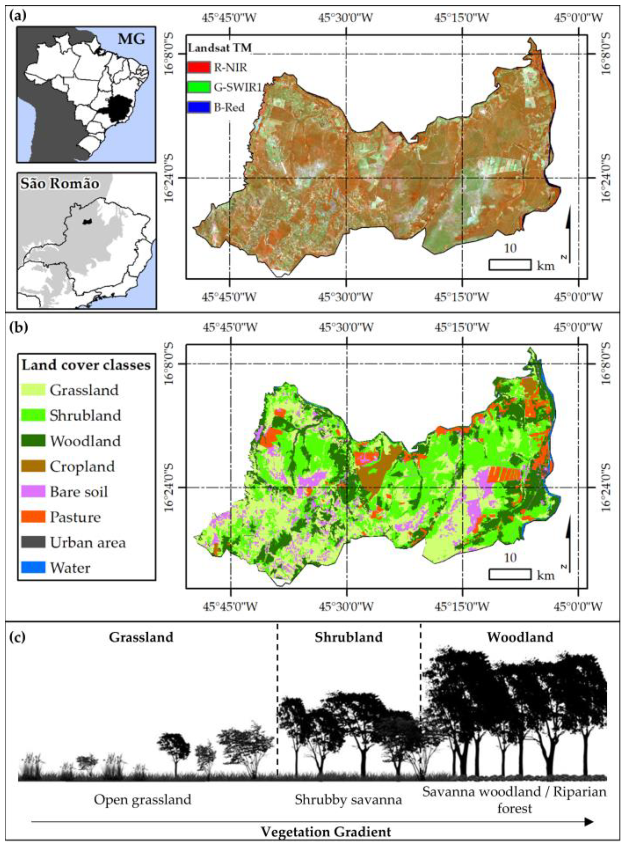
Figure 1. (a) The location of state of Minas Gerais (MG) in Brazil; São Romão shown in inset; map of Brazilian savannas biome and Landsat TM (Thematic Mapper) composite: Red-NIR (Near Infrared), Green-SWIR 1 (Shortwave Infrared) and Blue-Red; (b) Land-cover classes presented in the study area (adapted from [39]; (c) Savannas natural vegetation gradients (adapted from Reference [40]).
Remotesensing 10 00808 g001
Figure 2. The methodology flowchart detailing the three main steps to detect land cover changes over the savanna biome: 1. feature extraction from time series using NDVI trends at the object level; 2. Change detection using the random forest to model the change type as a function of Spatio-Temporal Metrics; 3. evaluation of change detection using accuracy measures.
Remotesensing 10 00808 g002
Figure 3. The Landsat TM Red-NIR, Green-SWIR 1 and Blue-Red composite. Examples of no-change class: (a) savannas affected by phenological effects; and forest change classes; (b) savannas undergoing a change by fire; (c) savannas undergoing a change by deforestation.
Remotesensing 10 00808 g003
Figure 4. The graphic representation of AFM (Area first lag—first maximum) index in the classical semivariogram: (σ2)—sill, (ϕ)—range, (τ2)—nugget effect, γ (h)—semivariance, γ max _ 1 —total variance, and γ1—semivariance at first lag.
Remotesensing 10 00808 g004
Figure 5. Example of Landsat time series from 2003 to 2016 of (a) average of NDVI values; (b) standard deviation of NDVI values; (c) RVF (Ratio variance—first lag) index; (d) AFM (Area first lag—first maximum) index; (e) comprising objects containing (i) seasonal changes and (ii) land cover changes.
Remotesensing 10 00808 g005
Figure 6. The three main steps to obtain the STM (Spatio-Temporal Metrics) from AFM (Area first lag—first maximum) time series to train the RF (Random Forest) algorithm: (a) Example of an object undergoing a forest fire and; (b) Example of an object relating the no-change class.
Remotesensing 10 00808 g006
Figure 7. (a) The location of training and validation samples of No-change and Forest change distributed over the study area; (b) example of an object undergoing a forest fire from August 2015 to October 2015; (c) example of No-change object over the entire time series (July 2003–October 2016).
Remotesensing 10 00808 g007
Figure 8. Examples of NDVI semivariogram: (a) During the wet season; (b) during the dry season; (c) impacted by fire; (d) their combination.
Remotesensing 10 00808 g008
Figure 9. The change maps for the 2003–2016 period generated by the features: (a) average; (b) standard deviation; (c) RVF index; (d) AFM index.
Remotesensing 10 00808 g009
Figure 10. The comparative analysis among the validation map and the estimates using (a) average spectral feature; (b) standard deviation spectral feature; (c) RVF semivariogram index and (d) AFM semivariogram index.
Remotesensing 10 00808 g010
Figure 11. The example of NDVI spatial variability of objects under a seasonal change and deforestation land cover change.
Remotesensing 10 00808 g011
Figure 12. Example of NDVI spatial variability of objects (a) under a seasonal change and (b) deforestation land cover change.
Remotesensing 10 00808 g012
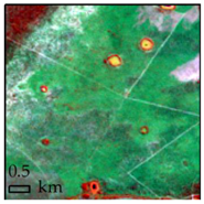
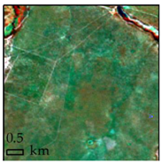
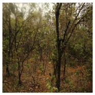
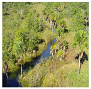
Table 1. The examples of the savannas land cover classes found in the study area. Landsat TM images Red-NIR, Green-SWIR 1 and Blue-Red composite.
Land Cover ClassesDescriptionField ViewLandsat TM Images
GrasslandsOpen grassland Remotesensing 10 00808 i001 Remotesensing 10 00808 i002
ShrublandsOpen grassland with sparse shrubs Remotesensing 10 00808 i003 Remotesensing 10 00808 i004
Savanna WoodlandsMixed grassland, shrubland, and trees up to seven meters Remotesensing 10 00808 i005 Remotesensing 10 00808 i006
Riparian forestsPalm swamps and Semideciduous forests Remotesensing 10 00808 i007 Remotesensing 10 00808 i008
Table 2. The image acquisition dates used to generate time series.
Sensor Type/Date (YYMMDD)Number of Scenes per YearSensor Type/Date (YYMMDD)Number of Scenes per Year
TM/200307046TM/200907045
TM/20030720TM/20090720
TM/20030821TM/20090805
TM/20030906TM/20090821
TM/20031008TM/20091125
TM/20031125
TM/200404016TM/201005046
TM/20040706TM/20100605
TM/20040823TM/20100621
TM/20040908TM/20100707
TM/20040924TM/20100824
TM/20041111TM/20100909
TM/200505064TM/201104213
TM/20050607TM/20110710
TM/20050725TM/20110912
TM/20050826
TM/200606265OLI/201304265
TM/20060813OLI/20130512
TM/20060914OLI/20130613
TM/20060930OLI/20130629
TM/20061117OLI/20130731
TM/200703097OLI/201402085
TM/20070426OLI/20140413
TM/20070629OLI/20140702
TM/20070731OLI/20140819
TM/20070901OLI/20141006
TM/20070917
TM/20071003
TM/200804286OLI/201506195
TM/20080514OLI/20150806
TM/20080530OLI/20151009
TM/20080717OLI/20151110
TM/20080802OLI/20151212
TM/20081005
OLI/201604183
OLI/20160707
OLI/20161027
Table 3. The geostatistical features: semivariogram indices [35].
IndicesDescriptionFormula
RVFRatio variance—first lag RVF = γ max _ 1 γ 1
AFMArea first lag—first maximum AFM = h 2 ( γ 1 + 2 ( i = 2 max _ 1 - 1 γ 1 ) + γ max _ 1 ) - ( γ 1 ( h max _ 1 - h 1 ) )
Table 4. The group of Spatio-Temporal Metrics (STM) used to train the RF (Random Forest) algorithm. The superscripted numbers are related to group names.
Group 1Group 2Group 3Group 4
STMDescriptionSTMDescriptionSTMDescriptionSTMDescription
Change 1Time series of NDVI AverageChange 2Time series of NDVI STDVChange 3Time series of RVF index Change 4Time series of AFM index
Trend 1Trend 2Trend 3Trend 4
Table 5. The classification scheme.
ClassesDescriptionTraining SamplesValidation Samples
No-changeAreas comprising the same cover in both epochs, albeit with changes caused by vegetation seasonality350150
Forest changeLand cover areas comprising deforestation and fires (savannas that were converted to bare soil and pastures)350150
Table 6. The classification results using groups of features tested. PA: Producer’s accuracy in %; UA: User’s accuracy in %; STDV: Standard deviation; RVF: Ratio variance-first lag; AFM: Area first lag-first maximum.
ClassesAverageSTDVRVFAFM
PAUAPAUAPAUAPAUA
No-change58.961.588.686.969.874.497.794.4
Forest change67.965.588.189.778.574.395.798.2
Overall accuracy63.788.374.496.5
Kappa coefficient0.30.80.50.9