1. Introduction
Behavior recognition of moving objects is a hot research topic in multiple fields, especially for surveillance and safety management purposes. In this paper, we focus on city road traffic where the basic road element is the vehicle object.
Studying the behavior of on-road vehicles at road intersections is a vital issue for building intelligent traffic monitoring systems and self-driving techniques. For example, in order to ensure safe driving, drivers need to know if the vehicles in front are going straight through the intersection or are making left or right turns. However, due to the crossing of multiple roads, crashes generally occur at intersections [
1]. In 2015, there were 5295 traffic crashes at four-way intersections with one or more pedestrian fatalities reported in the U.S. [
2]. Hence, intelligent transportation systems need to actively monitor and understanding the road conditions and give warnings of potential crashes or the occurrence of the traffic congestion.
Conventional behavior recognition systems rely on thousands of detectors (e.g., cameras, induction loops, and radar sensors) deployed on fixed locations with small detecting ranges to help capture various road conditions throughout the network [
3,
4,
5]. Such a system has exhibited many limitations in terms of range and effectiveness. For instance, if the information is required beyond the scope of these fixed detectors (i.e., blind regions), human labors are then frequently deployed to assess these particular road conditions [
6]. In addition, many monitoring tasks need to temporally detect detailed traffic conditions such as sources and destinations of the traffic flow, regions of incidents, and queuing information at crossroads [
7,
8]. To achieve this, visual information of multiple fixed detectors needs to be aggregated in order to provide a relatively large view of the area of interest, which could introduce extra noisy information and overhead costs. Therefore, it is essential to develop a more effective approach for acquiring visual information for further processing.
To tackle these issues, previous works have attempted to exploit still satellite images for traffic monitoring [
9,
10,
11]. Satellites can be used to observe wide areas, but they lack spatial resolution for specific ground locations. Additionally, data acquisition and processing are complicated and time-consuming, which hinders its application to real-time urban traffic monitoring tasks.
Thanks to the technological advances in electronics and remote sensing, Unmanned Aerial Vehicles (UAVs), initially invented for military purposes, are now widely available on the consumer market. Equipped with high-resolution video cameras, geo-positioning sensors, and a set of communications hardwares, UAVs are capable of capturing a wide range of road situations by hanging in the air or by traveling through the road network without restrictions [
12,
13,
14,
15]. Traffic videos captured by UAVs contain important information for traffic surveillance and management, and play an important role in multiple fields such as transportation engineering, density estimation, and disaster forecasting [
16,
17,
18]. However, UAVs are not widely applied in the vehicle behavior recognition system due to specific challenges for detecting and tracking vehicles in the UAV’s images and videos.
On one hand, the equipped camera of a UAV may rotate and shift during the recoding process. On the other hand, compared with conventional monitoring systems, the UAV’s video contains not only the ordinary data such as the global view of the traffic flow, but also each vehicle’s own data regarding, for example, its moving trajectory, lane changing information, and its interaction with other vehicles [
19,
20]. Therefore, the UAV’s video needs to be recorded using a very high resolution and frame frequency so as to capture adequate ground details. This inevitably leads to a huge amount of UAV video data and poses challenges for vehicle detection and tracking algorithms [
21].
To deeply understand city road vehicle behavior and overcome the challenges brought by real-world UAV video data, we developed a robust Deep Vehicle Behavior Recognition (DVBR) capable of recognizing different vehicle behaviors in high-resolution () videos. As a case study, we focus on vehicle behavior recognition at intersections.
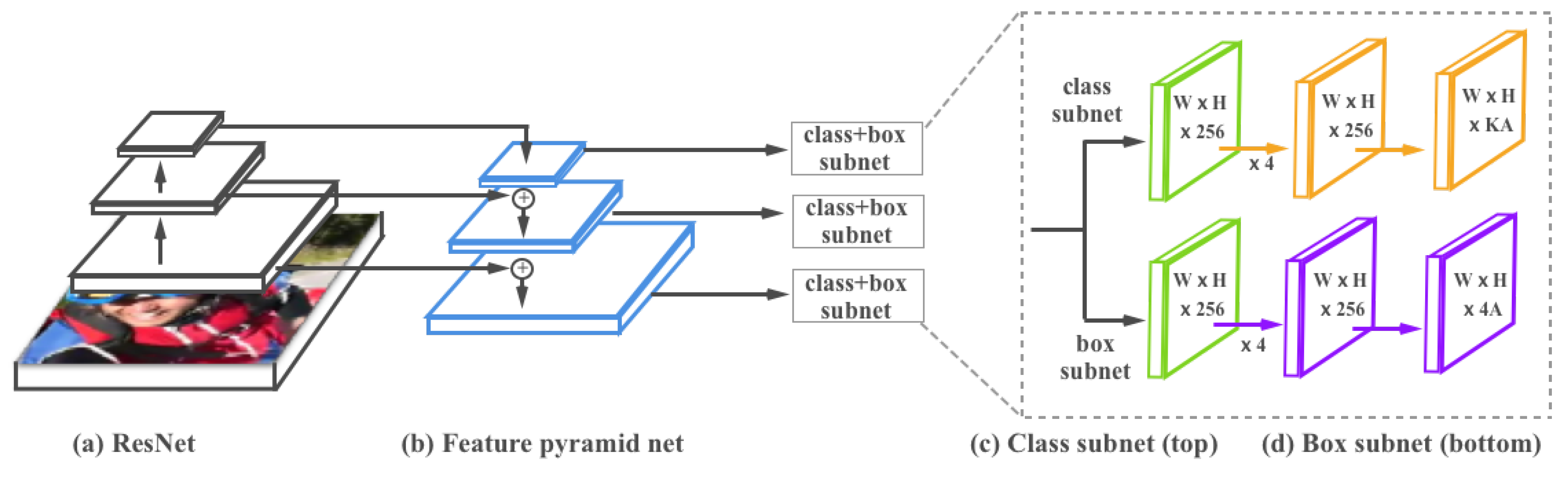
The DVBR framework contains two main parts: the first consists in vehicle trajectory extraction. More concretely, we first trained a Retina object detector [
22] to localize and recognize different vehicles (i.e., cars, buses, and trucks). Then we detected vehicles frame by frame on an input video, and developed a simple online tracking algorithm to associate detections across the whole video sequence. Based on the tracking results, we modeled and extracted vehicle trajectories from the original traffic video. To the best of our knowledge, this is the first framework which integrates deep neural networks and traditional algorithms for analyzing 4K (
) UAV road traffic videos.
The second part is vehicle behavior recognition. We approached this problem based on a nearest neighbor search and bidirectional long short-term memory, respectively. We conducted a comparative study in the experiments to demonstrate the effectiveness and superiority of proposed methods.
The rest of this paper is organized as follows.
Section 2 briefly discusses work related to vehicle behavior recognition.
Section 3 elaborates the Deep Vehicle Behavior Recognition Framework.
Section 4 presents experiment settings, results, and discussion.
Section 5 summarizes our work and discusses the path forward.
2. Related Work
Behavior recognition could be treated as the classification of time series data, for example, matching an unknown sequence to some types of learned behaviors [
23]. In other words, behavior recognition in traffic monitoring describes the changes in type, location, or speed of a vehicle in the traffic video sequence (e.g., running, turning, stopping, etc.).
In general, the behavior recognition system contains a dictionary constructed using a set of pre-defined behaviors, and then finds matches in the dictionary by checking each new observation of the vehicle behavior, e.g., slow or fast motion, heading north or south [
24]. Combined with the knowledge of traffic rules, these behaviors can be used for multiple applications, for instance, event recognition, which means generating a semantic interpretation of visual scenes (e.g., traffic flow analysis and vehicle counting), and abnormal event detection, such as illegally stopped vehicles, traffic congestion, crashes, red-light violation [
25], and illegal lane changing [
26].
Based on the vast amount of driving behaviors, there are two main approaches to understanding vehicle behaviors in road traffic scenes. The first one is vehicle trajectory analysis, and the other approach focuses on the explicit attributes of the vehicle itself, such as its size, velocity, and moving orientation.
2.1. Behavior Recognition with Trajectory
Many existing traffic monitoring systems are based on motion trajectory analysis. A motion trajectory is generated by tracking an object frame by frame in the video sequence and then linking its locations across the consecutive frames. In recent decades, various approaches to handle the analysis of the trajectory of moving objects based on city road traffic videos have been proposed. In [
27], a self-organizing neural network is proposed to learn behavior patterns from the training trajectories, and activities of new vehicles are then predicted based on partially observed trajectories. In [
28], the vehicle trajectories are modeled by tracking the feature points through the video sequences with a set of customized templates. Behavior recognition is then conducted to detect abnormal events: illegal lane changing or stopping, sudden speeding up or slowing down, etc. In [
29], the turning behaviors of road vehicles is detected by computing the yaw rate using the observed trajectories. Based on the yaw rate and modified Kalman filtering, the behavior recognition system is capable of effectively identify the turning behavior. In [
26], the lane changing information of target vehicles is modeled using the dynamic Bayesian network, and the evaluation is performed using the real-world traffic video data.
2.2. Behavior Recognition without Trajectory
Another way of recognizing behavior is to inspect non-trajectory information such as the size, velocity, location, moving orientation, or the flow of traffic objects [
30]. The main objective is to, according to this information, detect abnormal events of a moving target if the values of these attributes exceed the pre-defined value ranges. In vision-based road traffic analysis, speed is estimated by converting the image pixel-based distances to the absolute distances by manual geo-location calibration. By extracting velocity data, the traffic monitoring system is able to quickly detect congestion, traffic accidents, or violation behaviors. For example, Huang et al. use the velocity, the moving direction, and the position of vehicles to detect vehicle activities including sudden breaking, lane changing, and retrograde driving [
31]. Pucher et al. employ video and audio sensors to detect accidents such as static vehicles, wrong-way driving behaviors, and congestion on highways [
32].
To summarize, much work has been done on road vehicle behavior recognition, but most published results rely on small camera networks, which means their cameras only capture a small range of the traffic scene, and they focus on specific vehicle tracking and activity analysis. Additionally, many approaches simply treat road vehicles as “moving pixels”, while the types of road vehicles are often ignored. For example, they cannot process a query such as “find all illegally stopped cars on Southwest Road” or “find all trucks queueing at red lights to cross the road”. In our work, we use the UAV to capture a large area of the road traffic. Our vehicle detection and tracking algorithms are able to recognize different types of vehicles and maintain these unique identities for tracking.
4. Experiment and Discussion
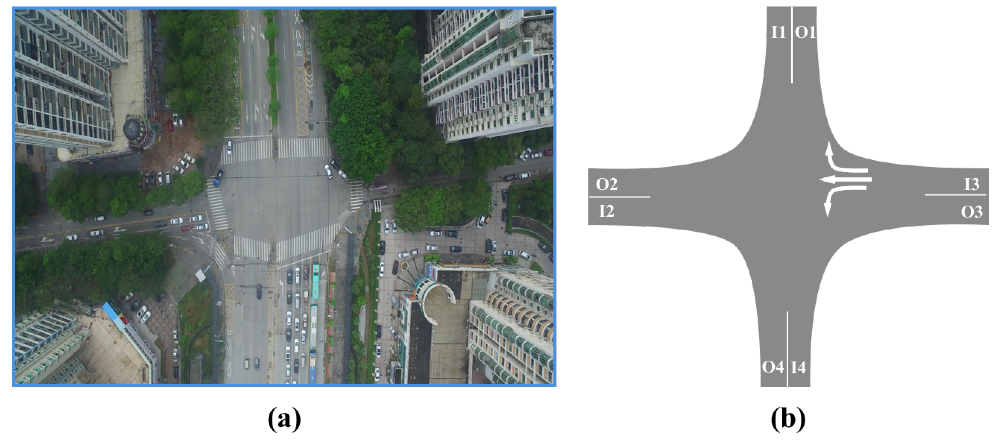
To evaluate the proposed framework, we captured a 14 m long traffic video with 4K resolution at a busy road intersections of a modern megacity by flying a UAV during the rush hours. The fps was 30 and the total number of frames was 25,200. The traffic scene at this intersection is shown in
Figure 7.
To build the training set, we first temporally subsampled the original video frames by a factor of 150. For each frame in the subset, we then divided it into small patches with a uniform size of . We allowed an overlapping area of 200 pixel vertically and horizontally between these patches to ensure each vehicle appeared as a complete object. We then obtained 3400 training images. Next, we manually annotate vehicles with the following information: (a) bounding box: a rectangle surrounding each vehicle; (b) vehicle type: three general types including car, bus, and truck. This yielded 10,904 annotated vehicles. We used this dataset to train the RetinaNet object detector.
For testing, we collected another short video at the same road intersection but at a different time. The length of the testing video is 2 m and 47 s, with a resolution and 30 fps. The total number of frames was 5010.
4.1. Vehicle Trajectory Extraction
4.1.1. Vehicle Detection
We conducted the vehicle counting experiment to evaluate the effectiveness of the RetinaNet for vehicle detection. More concretely, we counted all types of vehicles in a randomly selected frame from the testing video.
Settings. In the training phase, we randomly selected 85% of these training images for training and the remaining 15% for validation. We compared RetineNet with another three recent deep-learning-based object detection methods: the you-only-look-once version 3 (YOLOv3) [
46], the single shot multi-box detector (SSD) [
47], and the faster regional convolutional neural network (Faster-RCNN) [
48]. We trained the four deep models using Caffe [
49] toolkit on a GTX 1080Ti GPU with 11 GB of video memory. The optimizer was set to stochastic gradient descent (SGD) for better performance. We initialized the learning rate at 0.001, and it began to decrease to one-tenth of the current value after 20,000 epochs. The total number of epochs was set to 120,000, and the momentum was set to 0.9 by default according to these models.
In the testing phase, the testing image was first divided into small patches () with an overlap of 200 pixels, and these patches were then fed into the trained network to detect vehicles. The global result was obtained by aggregating detection results on all patches. We eliminated the repeated bounding boxes on each vehicle by setting the center distance threshold as 0.3 and the IoU threshold as 0.1, respectively (determined by cross validation).
Evaluation. To make vehicle counting more straightforward, the detection result was visualized by drawing vehicle locations and corresponding types on the input image. Counting was done naturally by measuring the number of these bounding boxes. We quantitatively evaluated the counting result via precision, sensitivity, and quality, which are defined in [
50]. True positives (TPs) are correctly detected vehicles, false positives (FPs) are invalid detections, and false negatives (FNs) are missed vehicles. Among the three evaluation criteria, quality is most important since it considers both the precision and the sensitivity of detection algorithms.
Result and discussion. We report the counting result on the testing image (see
Table 1). It can be seen that the RetinaNet achieves the best performance, followed by YOLOv3 and SSD. The Faster-RCNN method yields too many false negatives (missing vehicles), which leads to low sensitivity and quality scores.
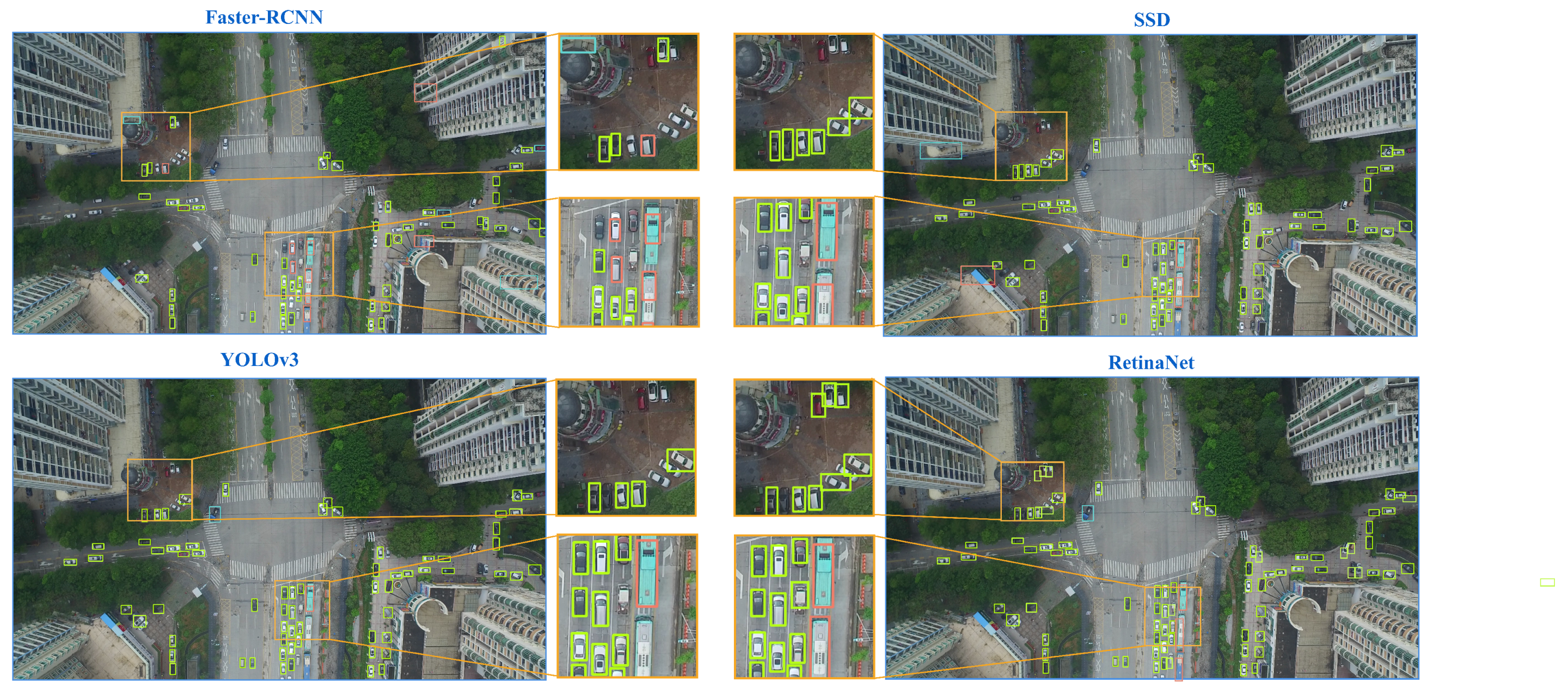
We visualize the results on the testing image (see
Figure 8). Cars, buses, and trucks (if any) are automatically marked with light green, orange, and light blue bounding boxes, respectively. The small images in the middle are patches extracted from the original images, which give clearer ground details for type-specific detection. We noticed that SSD and Faster-RCNN generate a small number of false positives. This is to be expected, because in the training set, only regions containing vehicles are annotated by human annotators, while non-vehicle areas (including pure background and empty road) are ignored. A few ignored regions may exhibit very similar appearances with particular vehicles (especially buses and trucks), which would consequently lead to a few wrong detections.
We also provide the training time and the testing speed (frame per second) in
Table 2. It can be observed that training of the Faster-RCNN model takes the longest time, but the testing speed is the lowest. The YOLOv3 model achieves the lowest training time and the fastest testing speed, which is due to its shallow network architecture compared with other models. However, its detection performance is worse than the RetinaNet model.
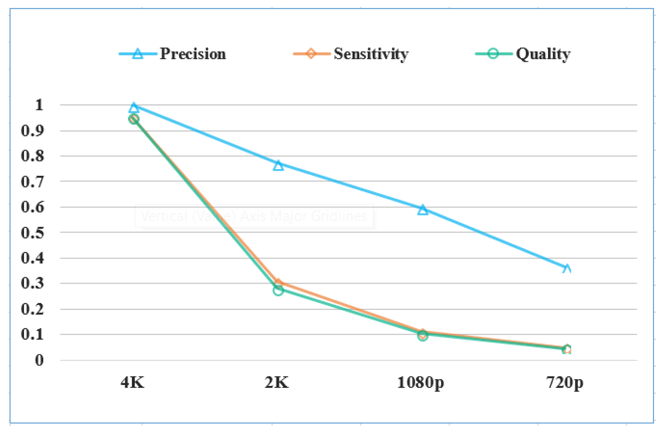
4.1.2. The Impact of Image Resolution
Although our data was recorded using 4K resolution, we are interested in determining if a high resolution really benefits the detection results. To do this, we created an auxiliary set where we down-sample the testing image. By adjusting the resolution of each image, we can determine performance changes of the detection algorithms. More specifically, we resized the original testing image to a resolution of 2K (2560), 1080p (), and 720p (), respectively. We then detected vehicles in these low-resolution images using the RetinaNet model.
The results are shown in
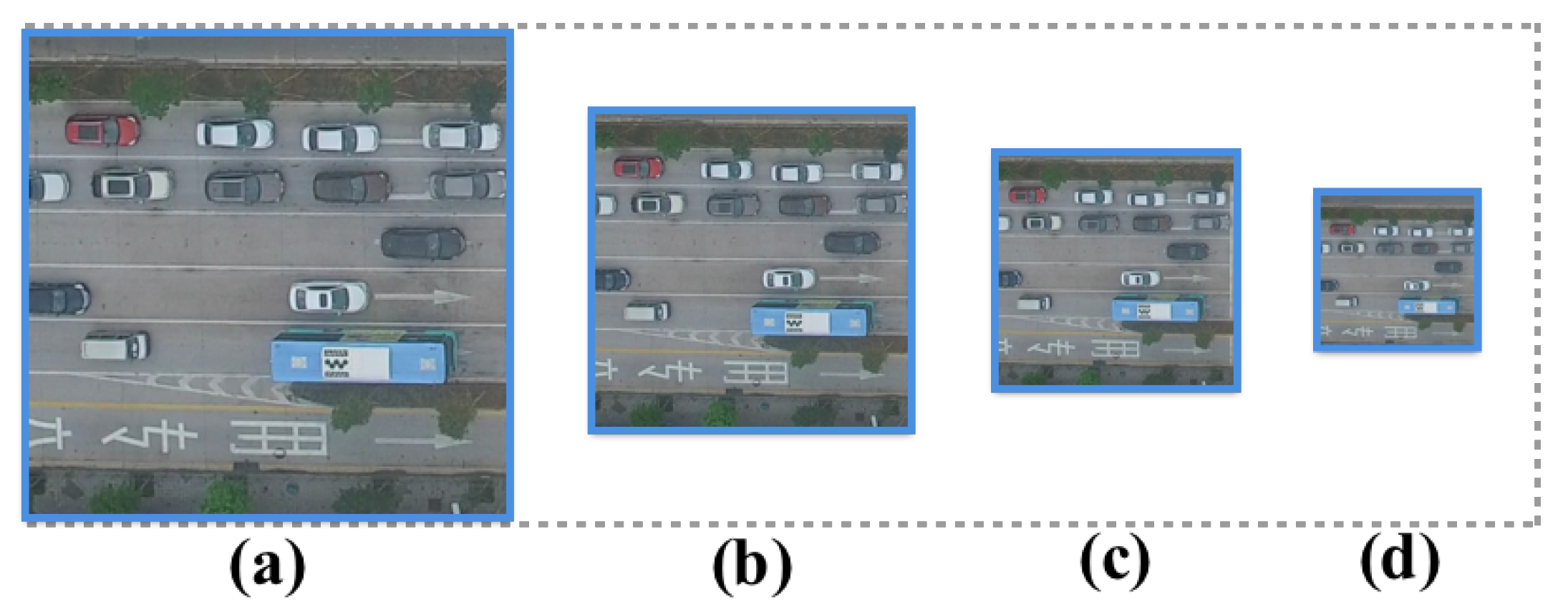
Figure 9. It can be seen that the detection performance degrades dramatically when the image resolution goes down, especially for the sensitivity measure and the quality measure. This makes sense because, in a 4K image, a vehicle generally takes a few pixels. However, in a 720p image, it only takes one or two pixels. This makes these vehicles (especially small cars) totally unrecognizable (see
Figure 10) for vision-based algorithms. Hence, recording data in a high resolution is necessary since it provides enough ground details to help the detection algorithms accurately localize different types of vehicles.
4.1.3. Vehicle Trajectory Modeling
Settings. We modeled vehicle trajectories according to the tracking results. Given the testing video, we performed frame-by-frame vehicle detection using the trained network. Once detection was complete, a set of trackers were created to associate bounding boxes with different vehicles across the whole video sequence. We empirically set the threshold as 0.3 to start a new track, and set as 10 to terminate a track.
During the tracking phase, vehicles which were not within the range of roads (e.g., parking lots) were ignored in the counting phase since they contribute nothing to estimate the city traffic density. We manually defined the road ranges, since testing videos contained large-range and complex traffic scenes. For implementation, we ran the tracking algorithm on the testing videos using an Intel i7-6700K CPU with 32 GB on-board memory.
Evaluation. To evaluate the performance of the trajectory modeling approach, we tracked the target vehicle in consecutive frames, and extracted the tracked center point
of its bounding box in each frame. For the
, we computed the trajectory modeling error between the tracked center point and the ground-truth center point (labeled by human annotators)
using
Based on Equation (
13), we can compute the overall error by adding the modeling error in each frame:
where
n is the number of frame being tracked. This error
E is quantified using the number of pixels, and it could be easily extend to the real value of centimeters by multiplying it by a factor of 10 (i.e., the ground resolution is 10 cm/pixel).
We tracked all vehicles in the testing video and extracted 238 complete trajectories. The trajectories with unknown types were ignored. We then randomly selected 50 vehicles and computed their trajectory modeling errors using Equation (
13). We took the average value as the modeling error of this frame. The modeling error of the whole testing video was then computed using Equation (
14).
Since our modeling method is based on vehicle tracking, we used three other recent tracking approaches to model the vehicle trajectory and evaluate their performance for comparison, namely, tracking-learning-detection (TLD) [
51], tracklet confidence and online discriminative appearance learning (TC-ODAL) [
52], and the Markov decision process (MDP) [
53]. In other words, our objective was to model the vehicle trajectories using the four methods and then evaluate their performance by computing the modeling error.
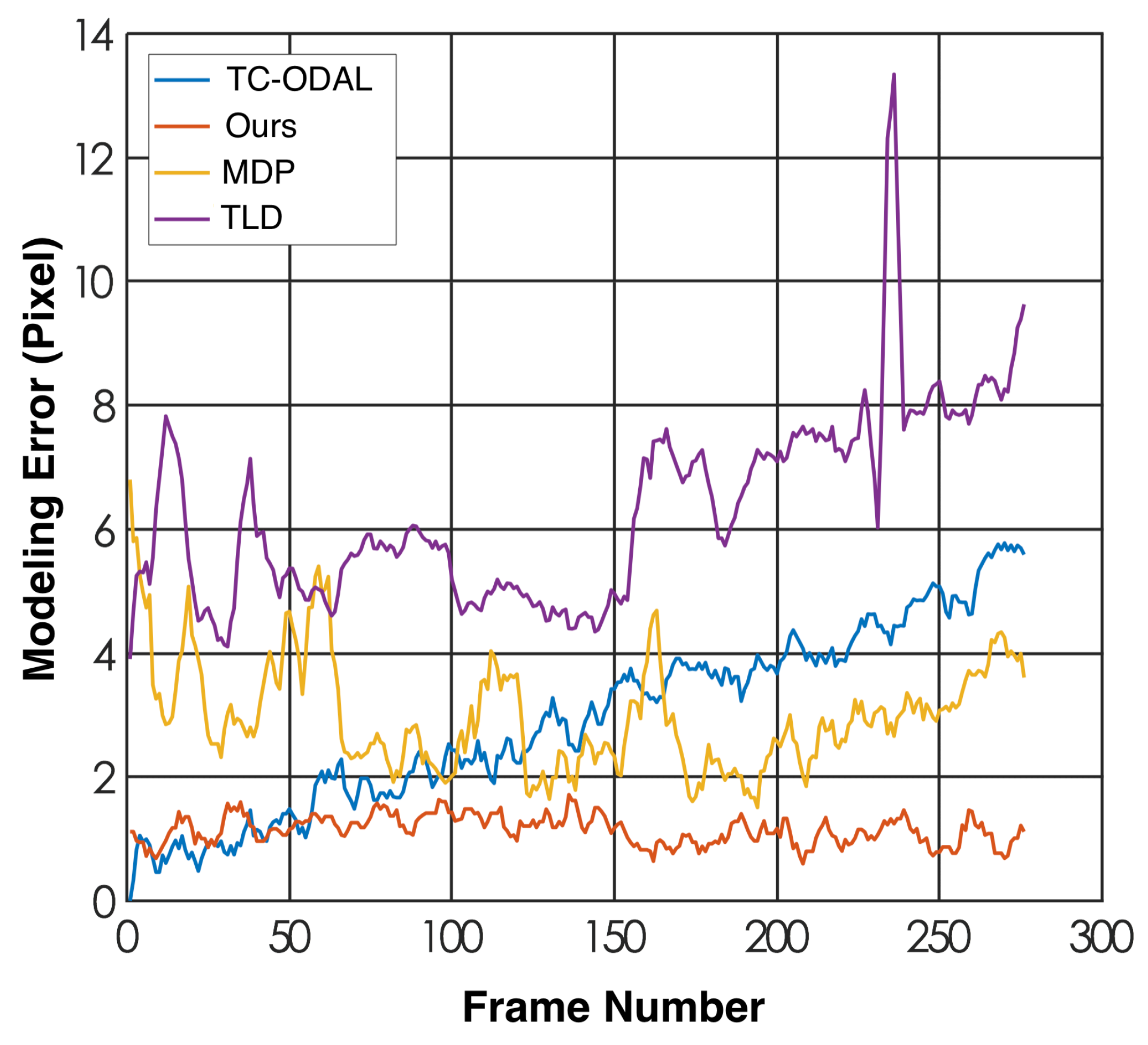
Result and discussion. We illustrate the frame-based trajectory modeling error for the first 280 frames of the testing video in
Figure 11 and report the overall error in
Table 3. It can be seen that our method outperformed the other three approaches in terms of both frame-based error and the overall error. The TLD method performed worst in this experiment, probably due to the lack of tracking information, since this method does not perform frame-by-frame vehicle detection on the video sequence. Fluctuations of the modeling error could be observed from the results of all four methods, but the error fluctuation range of our method was the smallest compared to the other three ones.
We also provide the tracking speed (frame per second) of the aforementioned approaches (see
Table 4). Since we already have the frame-by-frame detection results, we can treat the tracking problem as the data association problem and do not need to train the algorithm. It can be seen that all the approaches achieve a relatively high tracking speed (i.e., above 55 fps), and the proposed method achieves the highest speed (i.e., 82.5 fps) as well as the lowest tracking error.
4.2. Vehicle Behavior Recognition
4.2.1. Behavior Recognition by Nearest Neighbor Search
Settings. For training, we built a training set by extracting 973 complete vehicle trajectories from the training video. Five hundred forty-two of them were with the type “go straight”, 204 of them were with the type “turn left”, and the remaining 227 were with the type “turn right”. For testing, we used 238 trajectories obtained from the testing video.
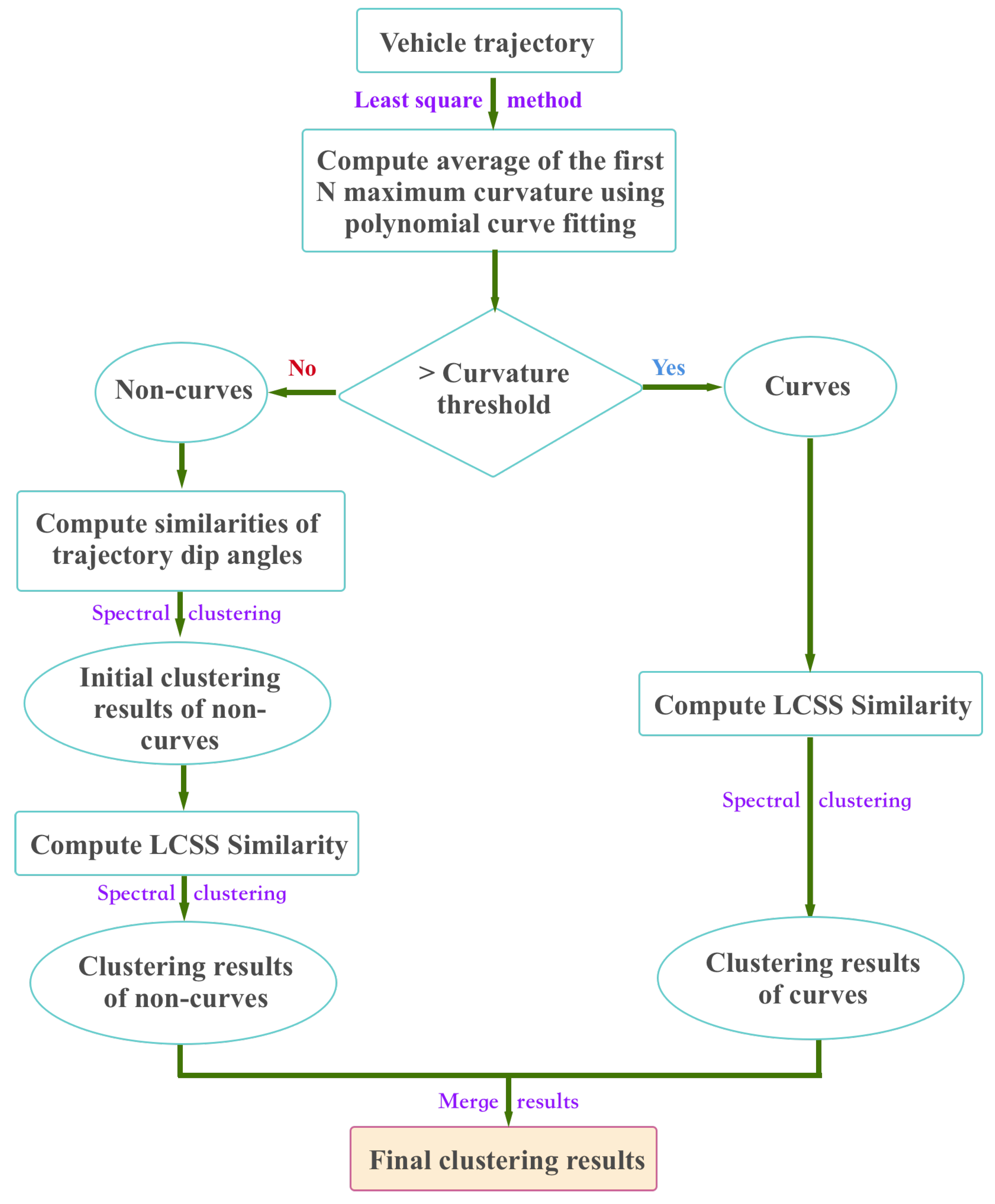
We applied the proposed double spectral clustering (DSC) on all the 973 trajectories and identified their types (i.e., go straight, right turn, and left turn). Given a testing trajectory, we determined its category based on a nearest neighbor search. We also performed two other clustering methods for comparison, one was a K-Means clustering based on LCSS similarity and the other one was normal spectral clustering based on LCSS similarity.
Evaluation. We employed the normalized accuracy metric considering the large variation in the number of samples in each trajectory type (most of them were of the type “going straight”). We first computed the accuracy within each class and then averaged them over all classes:
Result and discussion. The results are listed in
Table 5. We noticed that our approach achieved an overall accuracy of 0.899, which is pretty high considering the complex road structure. In addition, the recognition accuracy of vehicle going straight is 0.910, followed by the the accuracy of “left turn” and “right turn”, achieving 0.857 and 0.882, respectively. On each class, our DSC method outperformed the other two methods, which demonstrates the effectiveness of our approach for unsupervised vehicle behavior recognition.
The training time and testing speed of these three approaches are shown in
Table 6. It can be seen that the LCSS-KMeans runs faster than other methods, this is due to the relatively simpler complexity of the KMeans algorithm (the time complexity of KMeans is
, while the time complexity of spectral clustering is
). However, the performance of LCSS-KMeans is worse than the proposed DSC method. In addition, the three methods achieve a very similar testing speed, because they have roughly the same sizes of searching space.
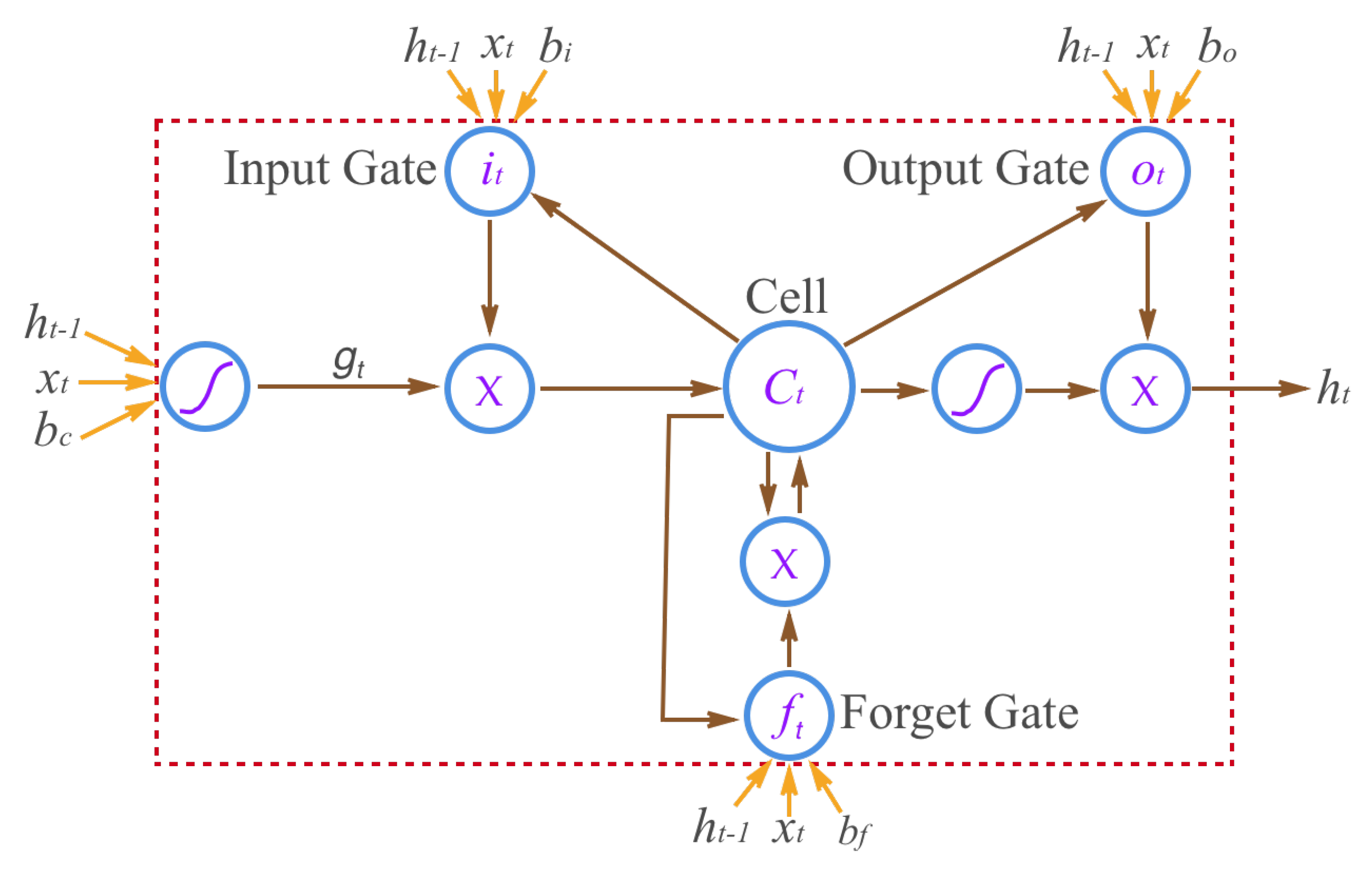
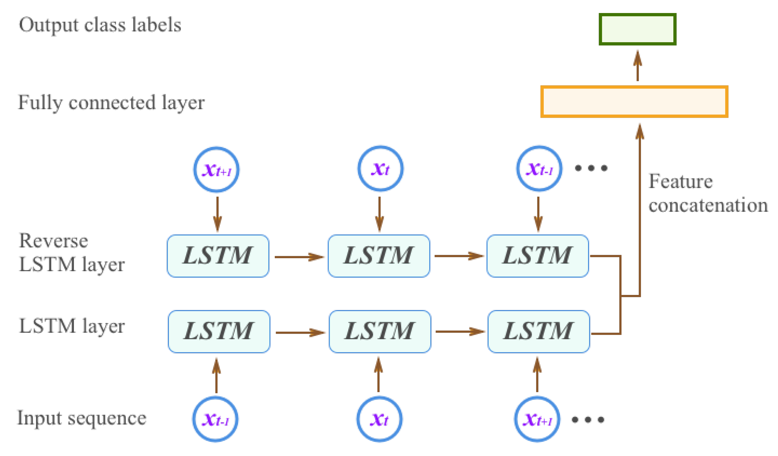
4.2.2. Behavior Recognition by Bidirectional Long Short-Term Memory
In this test, we performed behavior recognition using the proposed T-BiLSTM model.
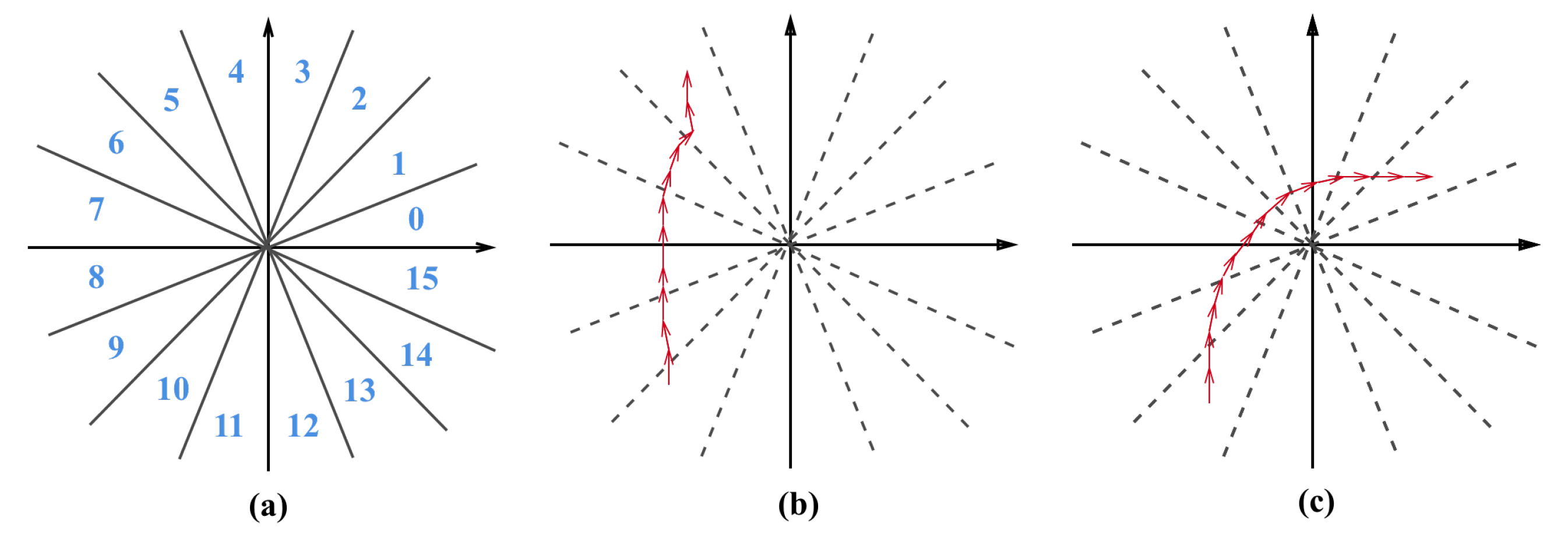
Settings. We used the same training and testing data as in the previous section. For feature representation, we resampled the length of each trajectory to 256 points, and computed the sequences of angular changes for them. We followed [
41] and employed the “back propagation through time” (BPTT) algorithm with a mini-batch size of 32 to train the network. For implementation, we used the Keras [
54] deep learning toolkit for Python using Tensorflow [
55] as backend.
For comparison, we trained five other models using our training data, namely a Hidden Markov Model (HMM) [
56], an Activity Hidden Markov Model (A-HMM) [
57], a Hidden Markov Model with Support Vector Machine (HMM-SVM) [
58], a Hidden Markov Model with Random Forest (HMM-RF) [
58], and normal LSTM [
59]. The first four algorithms were trained on the CPU (i7-6700K), while the normal LSTM and our method were trained on the GPU (GTX 1080Ti). For evaluation, we used the normalized accuracy metric again.
Results and discussion. Table 7 presents the classification accuracy of each method on the testing data. Our approach outperformed all other methods in terms of both single class performance and overall performance. To be more specific, our T-BiLSTM achieved an accuracy of 0.965 on the “go straight” types, probably because the structure of the trajectories under this type are relatively easy to be temporally modeled and recognized. The accuracies decrease on the other two trajectory types due to the increased structural complexity. The LSTM method achieves the second highest accuracy, followed by HMM-RF and A-HMM.
We also show the training time and testing speed of these methods in
Table 8. It can be seen that the training time of our method on the GPU is the lowest among the six trajectory classification approaches. For fair comparison, we also provide the training time of two deep-learning-based methods (LSTM [
59] and ours) on the CPU side, which is much lower than on the GPU side. For testing speed, the HMM achieves the highest speed, but its classification performance is significantly worse than our method.
5. Concluding Remarks
A deep vehicle behavior recognition framework is proposed in this paper for urban vehicle behavior analysis in UAV videos. The improvements and contributions in this study mainly focus on four aspects: (1) we expand the vehicle behavior analysis area to the whole traffic network at road intersections, not individual road sections; (2) to recognize vehicle behaviors, we propose a nearest-neighbor-search-based model and a deep BiLSTM-based architecture considering both forward and backward dependencies of network-wide traffic data; (3) multiple influential factors for the proposed model are carefully analyzed; (4) we combine deep-learning-based methods and traditional algorithms to effectively balance the speed and accuracy of the proposed framework.
In recent years, the rapid development of autonomous car technologies and driving safety support systems have attracted considerable attention as solutions for preventing car crashes. The implementation of technologies in the intelligent transportation system to assist drivers in recognizing driving behaviors around their own vehicles can be expected to decrease accident rates. Car crashes often occur when traffic participants attempt to change lanes or make turns. Hence, vehicle behavior recognition exhibits significant importance in our daily lives. In our work, we mainly use vehicle trajectory analysis to help recognize three types of vehicle behaviors, but vehicle trajectory analysis also has more applications which we will consider in future work: for example, illegal lane changes, violations of traffic lines, overtaking in prohibited places, and illegal retrograde. We will also implement an artificial-intelligence-based transportation analytical platform and integrate it into the existing intelligent transportation system in order to improve the driving experience and safety of drivers.


