1. Introduction
The power supply system is under fundamental transition. The replacement of fossil fuels by renewable energy is progressing rapidly. Weather-dependent energy sources such as wind and solar radiation play a major role within the transition. The integration of wind and solar energy into the grid has a huge impact on the load flows. For this reason, the forecasts of solar radiation and wind have to be more precise with particular regard to the short-term forecast for up to 3–4 h. Thus, a forecast based on satellite observations, also referred to as nowcasting, is of priority choice for this issue. It shows better results for the first few hours of photovoltaic power forecasts (PV forecasts) in comparison to numerical weather prediction models (NWP) [
1]. Further, NWP runs with data assimilation need usually 3–6 h of computation time. Thus, the results of the numerical weather prediction model are only available with a time delay of several hours, whereas satellite-based forecasts are available in near real time.
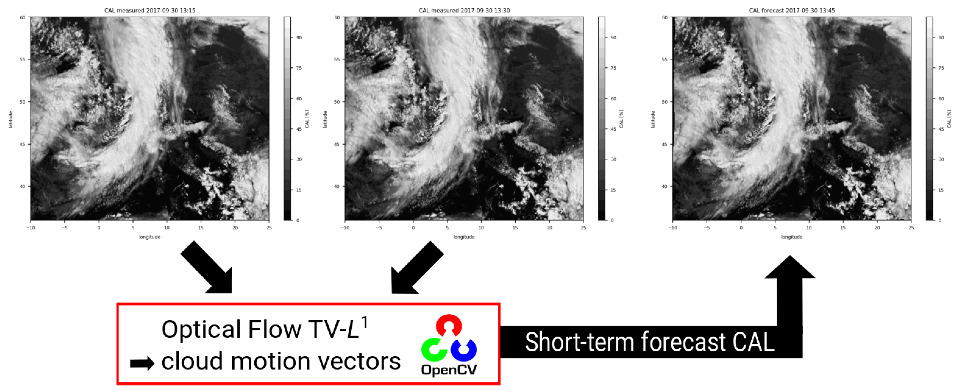
The temporal short-term variation of the solar surface irradiance in Central Europe is predominantly related to cloud occurrence. Thus, an accurate short-term forecast of relevant cloud properties is of high importance. The main challenge is to properly forecast the location and the shape of clouds for the next few hours from satellite data. For the forecast of clouds, we use the optical flow methods TV-
and Farnebäck provided by the OpenCV library through calculating cloud motion vectors [
2]. Optical flow is a widely-used and well-established technique for image pattern recognition in the fields of traffic, locomotion and face re-detection. An overview of different optical flow methods and their application is given by Sonka et al. [
3]. So far, however, TV-
and other optical flow methods are hardly used for the calculation of cloud motion vectors in meteorology. To our knowledge, one of the first applications has been the utilization of the optical flow for radar images as described by Peura and Hohti [
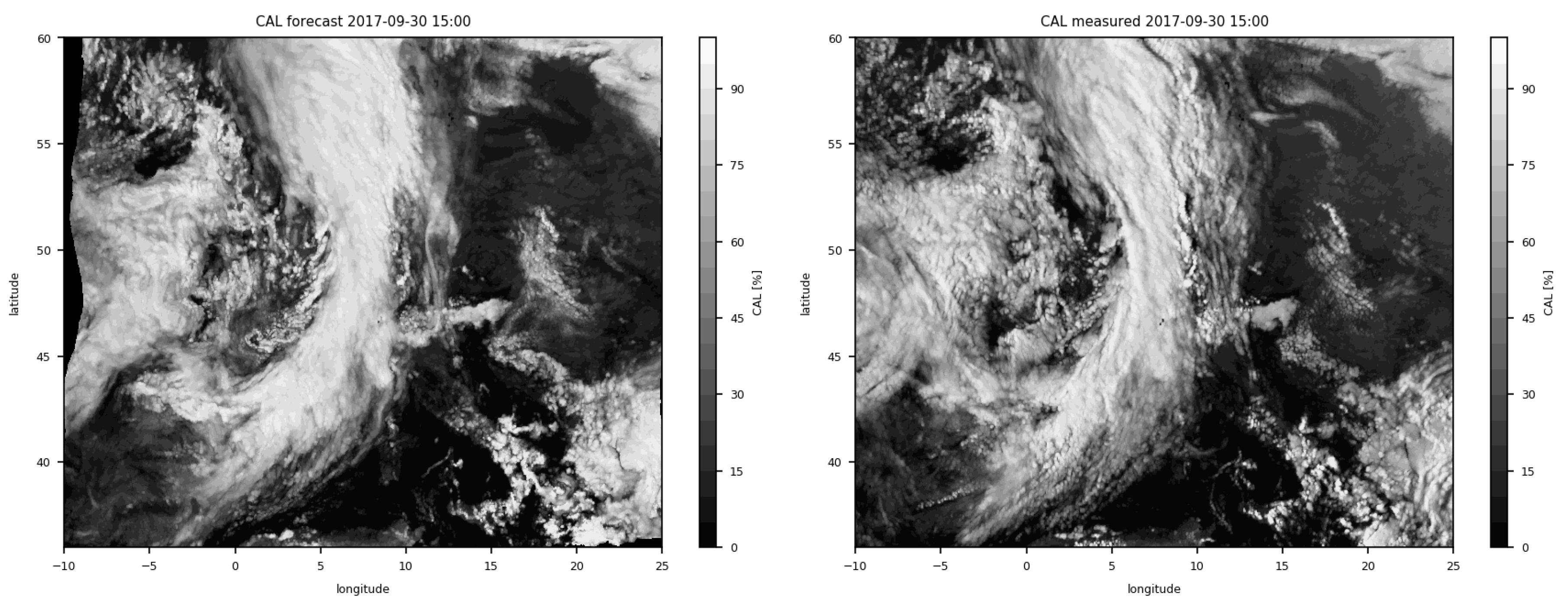
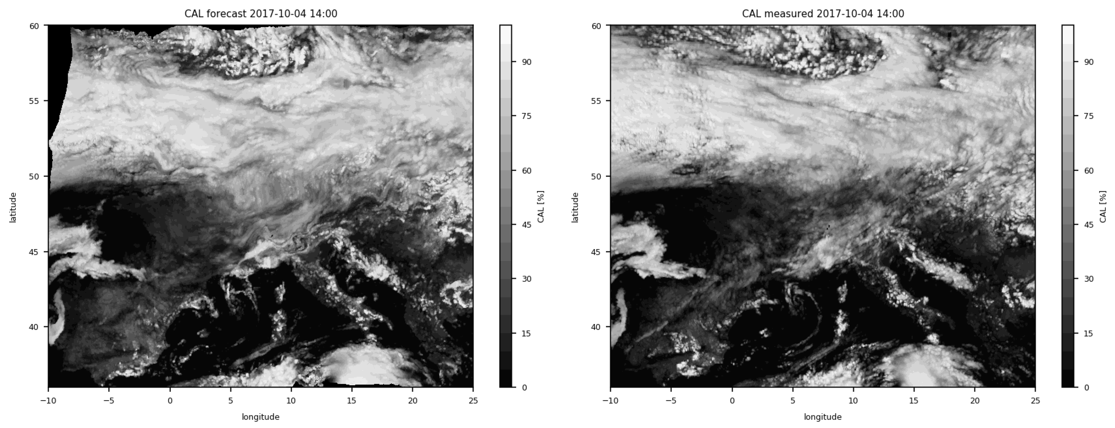
4]. Optical flow has been recently implemented for the short-term forecast of radar reflectivity at the German Weather Service (“Deutscher Wetterdienst”), as well. The success of the estimation of the optical flow of radar images indicates that the method could be transferred to the forecast of clouds and their properties. A promising candidate for the forecast of cloud properties is the effective cloud albedo (CAL). CAL is derived from the reflectivity measured in the visible bands of satellites. The advantages of the effective cloud albedo are manifold. For instance, CAL can be directly observed from space, without the need for any additional model or information [
5]. For CAL values up to 0.8, the cloud transmission for solar radiation is simply defined by
[
5]. Thus, the effective cloud albedo includes the required information about the cloud effect on the solar surface irradiance. Further, the reflection of the Earth’s surface is already filtered, allowing optical flow to focus on clouds. As a result, satellite observations enable the retrieval of the CAL and solar radiation at the ground, with high spatial and temporal resolution and a large areal coverage. For further information on the retrieval of the effective cloud albedo, the reader is referred to Müller et al. [
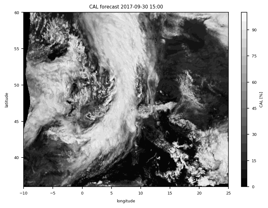
5]. In our study, the effective cloud albedo of two subsequent images is used as the input for the estimation of the optical flow method. The estimated cloud motion vectors are then applied on the latter of these two images to extrapolate the observed cloud albedo into the future. Further details on this topic are given in
Section 2.1.
Straightforward methods for the calculation of cloud motion vectors are based on the minimization of the root mean square error (RMSE) or the absolute difference between a shifted image in the x-y direction and the subsequent image. The cloud motion is defined by its shift in the x-y direction, which minimizes the RMSE or absolute difference between the images. This can be applied to various spatial scales and thus is called the multi-scale approach. Multiple scales lead to a dense vector field; however, more scales also increase the computation time needed. The cloud motion vectors applied for the satellite weather at the German Weather Service [
6] are an example of a straightforward multi-scale approach, which is based on the above-described minimization of the absolute differences. Another example is the method of Schmetz et al. [
7]. Here, a cross-correlation method is used for the cloud motion vectors. In this method, image filtering, also known as slicing, is applied to enhance the highest cloud tracer suitable for tracking. This filtering leads to a relative low density of cloud motion vectors, which is a significant disadvantage for energy meteorology applications. The Nowcasting Satellite Application Facility (NWCSAF) uses a similar approach, namely a gradient method, to define the cloud edges and cross-correlation for the calculation of the motion vectors [
8]. This method also leads to a low density of cloud motion vectors and is therefore not appropriate for energy meteorology. Originally, the main application of satellite-derived cloud motion vectors was the use of wind fields in the data analysis for numerical weather prediction where a dense field might be less important [
7]. However, only a dense field of cloud motion vectors enables a forecast with large geographical coverage and high temporal resolution without data gaps.
In the last few years, cloud motion vectors have gained significantly in importance within the scope of PV forecasts, and recently, their relevance has also been recognized for short-term forecasts of wind energy. However, a dense vector field of cloud motion vectors is a precondition for energy meteorology applications. Neural networks (NN) are therefore widely used to gain a dense vector field from high resolution satellite images with the advantage of a low computation time. Voyant et al. [
9] provide a review of neural network methods applied to the forecast of solar surface radiation. A disadvantage of neural networks is their black box character. A neural network is, strictly speaking, only valid for the training framework, as only the behavior of the training datasets can be reproduced. An application to other regions, periods or satellite instruments typically requires extensive re-training. Further, the black box character hampers a deeper understanding of the involved physics and physical reasons of the uncertainties occurring.
Thus, optical flow methods might be a good alternative for the estimation of cloud motion vectors. However, they are not mentioned neither in the review of photovoltaic power forecasting performed by Antonanzas et al. [
10], nor by the review of very short PV forecasting with cloud modeling by Barbieri et al. [
11]. Other leading experts, for example Raza et al. [
12], Perez et al. [
13] or Wolff et al. [
1], do not mention optical flow methods provided by OpenCV as an option for cloud forecasting. However, the optical flow of satellite images has been used for the Geometric Accuracy Investigations of the Spinning Enhanced Visible and Infrared Imager (SEVIRI) High Resolution Visible (HRV) Level 1.5 Imagery [
14]. Further, Simonenko et al. [
15] discussed the optical flow method TV-
concerning the interpolation between observed cloud images, in order to improve the temporal information about convective volcanic ash plumes. However, neither the short-term forecast of solar surface irradiance, nor its application were addressed. As a consequence, only a few works about the application of optical flow methods for the forecast of cloud motion vectors from satellite imagery and practically no works on satellite based short-term forecast of solar surface irradiance exist. Yet, the authors are aware of only one publication in which a multiple-scale optical flow method is applied within the scope of satellite-based solar irradiance forecasts [
16]. The respective method is developed within the storm detection and nowcasting system Cb-TRAM (Tracking and monitoring severe convection from onset over rapid development to the mature phase using multi-channel Meteosat-8 SEVIRI data) [
17,
18]. Unfortunately, the details of the method are not well described, and the software is not available in open access, which limits the scientific benefit of the work. Further, the authors applied the cloud motion vectors to cloud optical thickness and effective radius, but not to CAL. For the correct retrieval of cloud optical depth and effective radius
, accurate information of the surface albedo and the atmospheric composition is needed. Furthermore, simplifications in the radiative transfer are typically applied within the retrieval of the cloud optical depth and
. These items induce uncertainties in the estimation of the solar surface irradiance, which can be avoided if the satellite-observable CAL is used.
Thus, to the knowledge of the authors, the optimization of the recent TV-
method and its application to the effective cloud albedo for the forecast of solar surface irradiation is a novel approach within energy meteorology. Furthermore, this work is one of the first in which the two optical flow methods of the OpenCV library (TV-
, Farnebäck) are evaluated and compared in the context of cloud albedo forecasting. The authors believe that the combination of the effective cloud albedo with TV-
and SPECMAGIC NOW [
19] delivers a new powerful method for the short-term forecast of solar surface irradiance.
4. Discussion
The applications of optical flow estimates are diverse. As shown in
Section 3.3, the utilization of the optical flow estimation for a short-term forecast of the effective cloud albedo and hence of the solar surface irradiance shows promising results. Validation results reported in recent review publications by Voyant et al. [
9], Antonanzas et al. [
10] or Barbieri et al. [
11] and publications by other leading experts (Raza et al. [
12], Wolff et al. [
1], Cros et al. [
33]) do not provide any hints that the application of the widely-used neural networks leads to a significantly better accuracy for cloud motion vectors. In Cros et al. [
33], for example, the RMSE of the 30-min forecast of the effective cloud albedo was about 30% for a neural network approach and a phase correlation method. Thus, the discussed optical flow method might be among the best approaches for cloud motion vector estimation. Moreover, the big advantage of the TV-
approach, which has been optimized here for the effective cloud albedo, is the free access and the comprehensive documentation of the method. However, no matter which satellite-based method for cloud motion vectors is used, the limit of a good short-term forecast compared to NWP is approximately between 120 and 240 min because the forecast is only based on the optical displacement of pixels. The method does not lead to good forecast results after a certain time threshold. Comparisons with the numerical weather prediction models will be conducted in the future to provide more detailed information about the time when the accuracy of the NWP matches that of TV-
. Further, we plan to investigate the benefit of rapid scan imagery, which are available every 5 instead of 15 min.
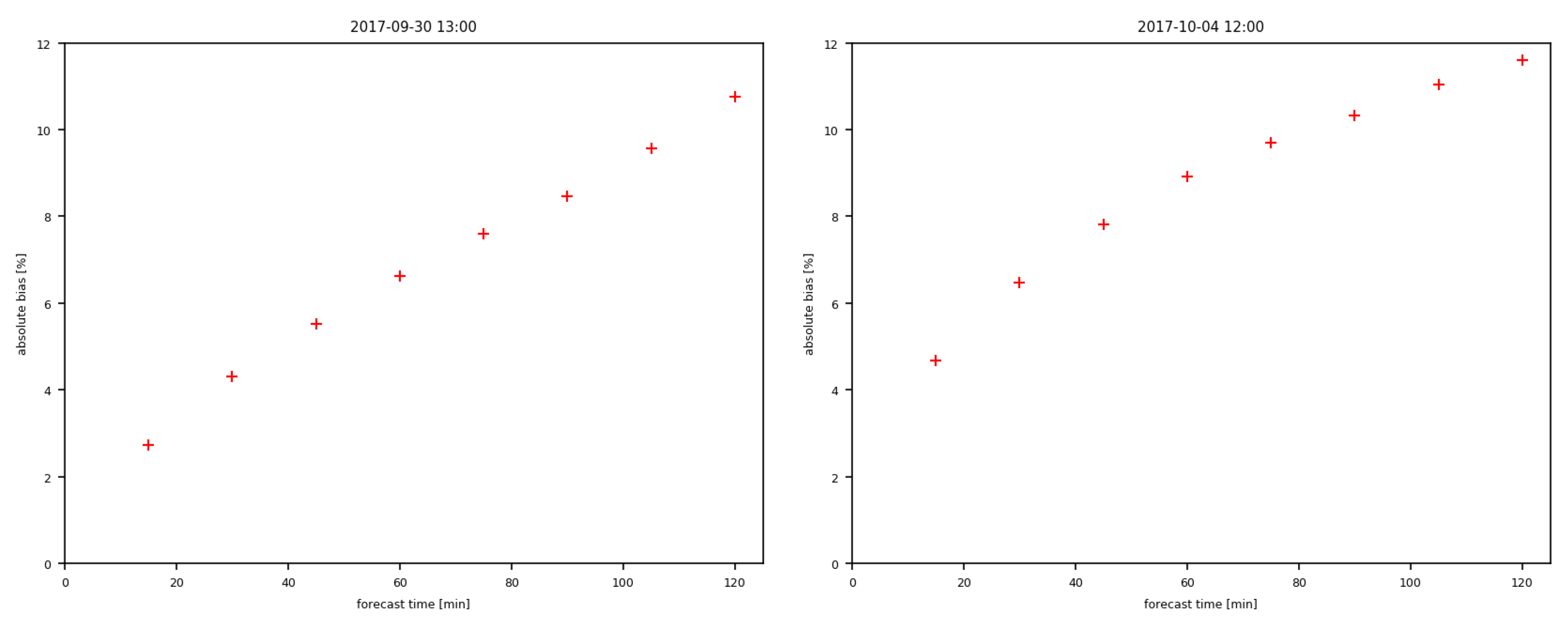
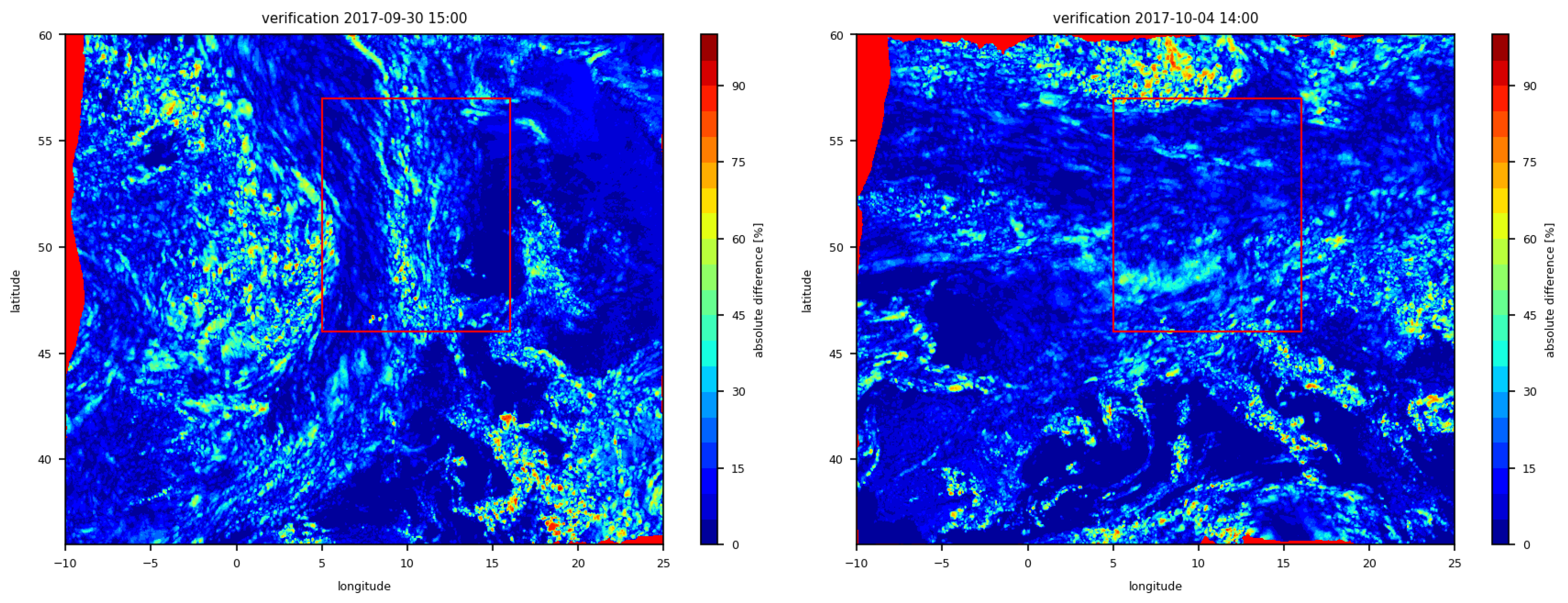
A currently known problem of satellite imagery methods is the formation or dissipation of clouds in the forecast, which can be caused for example by fast processes such as convection. This is confirmed by our verification results (see
Figure 7). As mentioned above, one criterion of the optical flow is that the intensity of image pixels has to stay constant between two consecutive frames. Due to the fact that convective clouds form very fast, this is clearly not fulfilled. Nevertheless, these areas where convection can be found are very small in comparison to stratiform clouds or fronts and, thus, are rather negligible for renewable energy forecasts. A common approach for short-term forecasts is the separation into sub-scales. Convection is a fast small-scale process, while pressure systems with fronts can extend up to 1000 km and exist for days. To cover both regimes, the optimization process can be done for the first 60 min and the second 60 or more minutes. This was already conducted for the 21 cases mentioned, but it did not improve the forecast. From 21 cases, there were only four in which a separate optimization would be useful. Besides, the differences between the optimal and the second best parameter value are in the range of hundredths and thus negligible. The implementation of such a parameter change would just be too costly.


