1. Introduction
By precise point positioning (PPP) [
1], centimeter-level positioning accuracy with only a single receiver is achievable. PPP has been recognized as a powerful and efficient tool for many applications, including geophysics and meteorology [
2,
3,
4]. While PPP has numerous advantages, it still takes approximately 30 min to achieve positioning solutions within accuracy of 10 cm. In addition, when compared with relative positioning, PPP suffers from relatively poor precision for observations covering a short time period.
In relative positioning, precise positioning can be achieved instantaneously using ambiguity resolution. In PPP, however, the uncalibrated phase delays (UPDs) [
5], or alternatively, the fractional-cycle biases (FCBs) [
6] are absorbed into the undifferenced ambiguity estimates; their integer properties are thus destroyed and therefore cannot be fixed. Fortunately, recent studies have demonstrated that suitable integer resolutions can be achieved through application of improved satellite products in which the FCBs have been separated from the integer ambiguities [
5,
7,
8,
9]. While major achievements have been reported with regard to ambiguity-fixed PPP, the PPP technique still requires long convergence times of 30 min or more to obtain centimeter-level positioning accuracy or to produce its first ambiguity-fixed solution [
10]. Such long convergence times are not acceptable for a wide range of applications.
Recently, some researchers proposed use of the Global Navigation Satellite System (GLONASS) to help with global positioning system (GPS) PPP ambiguity resolution. Jokinen et al. [
11] studied the initial fixing time (IFT) improvements by adding GLONASS observations to help with GPS PPP ambiguity resolution, in which only the GPS ambiguity is fixed and GLONASS is left floating. Their results showed that the addition of GLONASS can reduce the IFT by approximately 5% when compared with GPS-only solutions. Li and Zhang [
12] performed a similar analysis and found that the average IFT could be shortened by 27.4% in static mode and by 42.0% in kinematic mode. Later, other researchers analyzed the effects of simultaneous fixing of the GPS and GLONASS ambiguities; the results of Geng and Shi [
13] showed that the fixing percentage within a 10-min period for kinematic PPP improved from 39.81 to 87.50%, while a similar improvement from 46.8 to 95.8% was reported by Liu et al. [
14].
The BeiDou Navigation Satellite System (BDS) has been independently constructed and operated by China and has provided an official service in the Asia-Pacific region since 27 December 2012. The BDS satellite constellation is currently composed of five geostationary Earth orbit (GEO) satellites, five inclined geosynchronous satellite orbit (IGSO) satellites and four medium Earth orbit (MEO) satellites. Given the availability of precise clock and orbit products for the BDS satellites, it is therefore necessary to investigate the GPS + BDS PPP ambiguity resolution performance. It was shown in [
15,
16,
17] that the convergence time of float PPP can be reduced by combining the observations from the BeiDou satellites. Liu et al. [
18] showed that the fixing percentage for GPS-only kinematic precise point positioning integer ambiguity resolution (PPP-IAR) was 17.6% within a 10-min period, and this percentage improved to 42.8% following the addition of the IGSO and MEO satellites of the BDS. However, the fixing percentage degraded severely to 23.2% if the GEO satellites were included because of their low orbit accuracy. Researchers have performed large numbers of studies on precise orbit determination and precise positioning of the BDS [
19,
20,
21,
22,
23,
24]. However, because of the lack of sufficient numbers of tracking stations and a suitably precise solar radiation pressure model, the precision of the BDS orbit is low when compared with that of the GPS satellites, particularly for the GEO satellites, which have orbit errors of the order of 2–4 m. The Centre National d’Études Spatiales (CNES) has been providing real-time orbit and clock corrections for all global navigation satellite systems (GNSSs) since 2016. Kazmierski et al. [
25] analyzed the quality of the CNES’s real-time orbit by comparing it with that of the final product from the Center for Orbit Determination in Europe (CODE) [
26]. The results showed that GPS has the highest orbit precision of 2.3, 3.2, and 2.8 cm for its radial, along-track and cross-track components, respectively. For the BDS, the precision results for the three corresponding components were 12.1, 21.2, and 26.2 cm for the IGSO satellites and 4.8, 13.1, and 10.8 cm for the MEO satellites, respectively. To improve the precision of ultra-rapid orbits, Li et al. [
27] used two days’ worth of data to perform multi-GNSS ultra-rapid orbit determination, and updated the orbit results every hour. The results showed that when compared with the traditional strategy, the overlap accuracies of the BDS GEO, IGSO, and MEO satellites can be improved by more than 50, 18, and 44% in the radial, cross-track, and along-track directions, respectively, and the root mean square (RMS) values are summarized in detail in
Table 1.
As shown in
Table 1, the accuracy of the BDS ultra-rapid orbit is very low and thus cannot satisfy the FCB estimation requirements. In this paper, we propose a new strategy for BDS FCB estimation in real time. We begin by addressing the fundamentals of simulated real-time PPP data processing. We then demonstrate how the satellite orbit will affect narrow-lane FCB estimation and provide a new narrow-lane FCB estimation strategy that takes satellite orbit errors into consideration. We use a network of 60 tracking stations to validate the proposed method. Finally, discussion and concluding remarks are presented based on our findings.
2. Methods
The well-known ionosphere-free (IF) combination is commonly used in satellite clock estimation and PPP processing to eliminate the first-order ionosphere delay. The IF carrier-phase and pseudorange observations between the satellite
and the receiver
can be written as:
where
.
and
are the code and carrier phase observations, respectively, at frequency
.
is a nondispersive delay that includes the geometric delay, the tropospheric delay, and any other delay that has an identical effect on all observations.
and
are the receiver and satellite clock biases, respectively.
is the speed of light in a vacuum.
denotes the ambiguity of the IF carrier-phase observation.
is the satellite orbit error mapped into the receiver-satellite direction, which is typically assessed using signal-in-space ranging error (SISRE) values [
28]. The satellite-induced code bias (SICB) of the BDS must be corrected using e.g., the model reported by Wanninger and Beer (2015) [
29]. Note that the GEO satellites can be corrected using the same model that is used for the IGSO satellites [
30]. Finally,
and
denote the unmodeled code and carrier phase errors, respectively, which include multipath effects and noise. Both the phase center correction and the phase windup effect [
1,
2,
31] must be considered during the modeling process.
All real-time processes in this study are based on Equation (1). First, we fix the ultra-rapid orbit to enable estimation of the satellite clocks using a forward Kalman filter. To simulate a real-time scenario, we used the latest predicted orbits with 3 h of release latency. These clocks and the predicted orbits were then fixed as shown in the subsequent FCB estimation. Geng et al. [
32] and Shi and Gao [
33] have previously proved that the current PPP ambiguity resolution methods are equivalent in theoretical terms. Therefore, in this study, we focus solely on the method that was proposed by Ge et al. [
5], in which the FCB determination is critical. Finally, the satellite’s orbit, clock and FCB products are broadcast to all PPP users with a simulated latency of 3 s to assess the PPP-IAR performance.
2.1. Effects of Orbit Error on FCB Estimation
To generate the satellite FCB in PPP analysis, the satellite orbit and clock are fixed, which means that the orbit error is not separable from the IF ambiguity, and the second equation from Equation (1) will become:
where
. The corresponding IF ambiguity can be expressed using a combination of the wide-lane (WL) and narrow-lane (NL) ambiguities for fixing:
where
and
are the WL and NL ambiguities, respectively, which have corresponding wavelengths of
and
.
and
are the receiver and satellite NL UPDs, respectively, and
is the NL orbit error.
In PPP, the WL ambiguity is usually resolved using the Hatch–Melbourne–Wübbena (HMW) combination [
34,
35,
36] of the carrier phase and code observations as follows:
where
is the integer WL ambiguity, and
and
are the receiver and satellite WL UPDs, respectively. The advantage of this approach is that it is not affected by atmospheric (ionosphere and troposphere) bias or any geometry-related bias. Therefore, it will not be affected by the orbit errors.
In high-precision satellite clock estimation, part of the orbital error can be compensated by the satellite clock, while the residual part will appear as code residuals or can be absorbed into the float IF ambiguity in PPP, which then goes into the NL ambiguity, as shown in Equation (3). According to Liu et al. [
37], the proportion corresponding to the residual orbital error is governed by the term
, which is called the scale factor. Here,
represents the maximum value of the included angle between a vector from the satellite to one receiver and another vector from the same satellite to another receiver. The tracking network used in China covers an area with a radius of approximately 1500 km, and we can thus calculate the scale factor; then, based on the 3D orbit error given in
Table 1, we can also calculate the effects of the residual orbital error on the NL ambiguity. The resulting values are summarized in
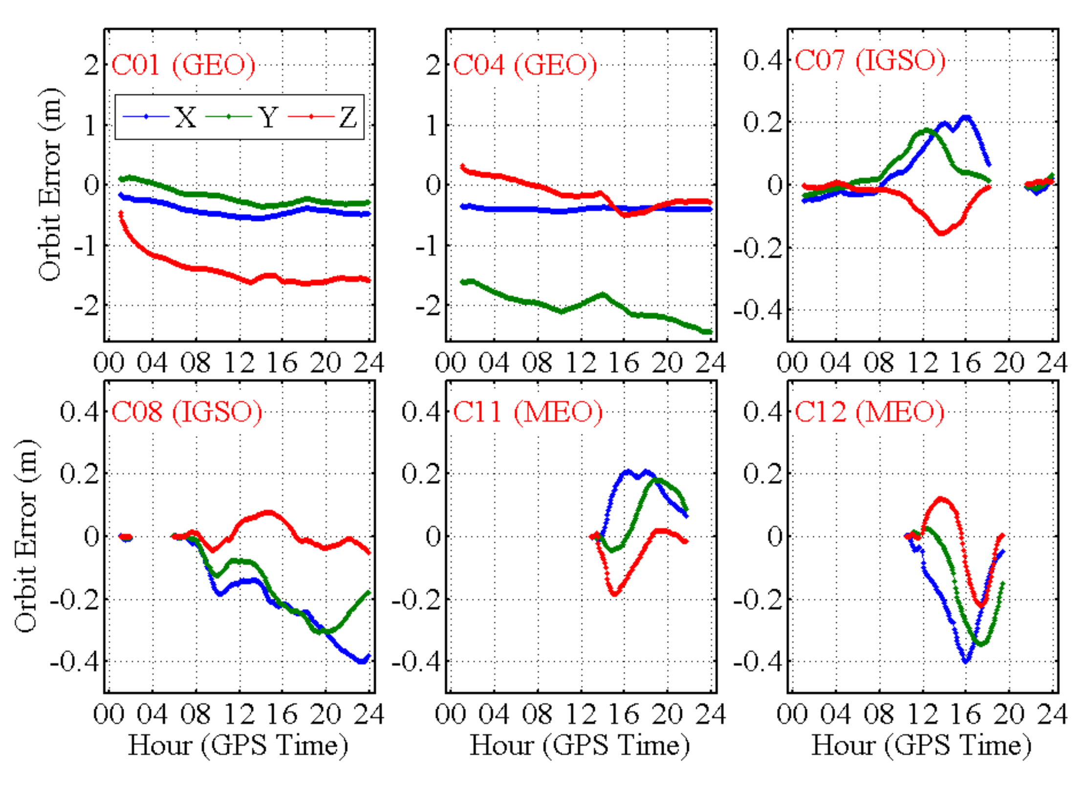
Table 2. The results show that the orbit errors of the GPS satellites can be neglected, whereas the orbit errors of all three types of BDS satellites must be estimated along with the NL FCB parameters.
After the WL ambiguities are fixed, the float NL ambiguities can then be obtained using Equation (3):
The orbit error is expressed as:
where
,
, and
are the satellite errors expressed in an Earth-centered and Earth-fixed coordinate system; and
,
and
are the corresponding direct cosines of the satellite.
To generate the GPS + BDS FCBs in the PPP analysis, the estimated parameters required include two receiver clock parameters, one zenith tropospheric delay (ZTD) parameter, and the undifferenced IF ambiguities. Based on the results given in
Table 1, we can neglect the GPS orbit error; we therefore assign much less weight to the BDS observations so that the precision of both the ZTD parameter and the GPS receiver clock will not be affected by BDS orbital errors. The slant orbital error will therefore be absorbed by the BDS receiver clock and the IF ambiguities; the former can be compensated by estimation of the BDS receiver’s NL FCB parameter. We can thus ensure that, based on Equation (5), the BDS orbit error can be retained along with the NL FCB estimates from the IF ambiguities.
2.2. FCB and Orbit Error Estimation Algorithm
Assume that there are
stations that observe
satellites in a network; then, based on consideration of Equation (5), we obtain the observation equation in the form of Equation (7) for all NL ambiguities in the network as follows:
where
represents the float ambiguities for receiver
and
stands for the corresponding integer ambiguities;
and
are the receiver and satellite FCBs, while
and
represent the corresponding design matrices, respectively;
,
, and
are the orbit errors, and
,
, and
are the corresponding design matrices, respectively. If we can fix all integer ambiguities in Equation (7), then the NL FCBs and the satellite orbit errors can be estimated together using the least mean squares (LSQ) adjustment method.
The orbit error may be very large, particularly for the GEO satellites (see
Table 3), and we have no a priori values, which means that it is impossible to fix all the ambiguities in Equation (7) for all stations in a straightforward manner. In this study, we propose an improved strategy to fix the ambiguities in Equation (7), which is detailed as follows:
- (a)
Add a loose zero-value constraint to all the orbit error and FCB parameters to eliminate the singular values in Equation (7). The variance of this constraint is set at 10 m in this study.
- (b)
Generate independent baselines among all the reference stations. For each baseline, assuming the initial satellite orbit error to be zero, form double-differenced (DD) NL ambiguities and then attempt to fix these DD ambiguities by rounding.
- (c)
Solve Equation (7) to obtain the updated satellite orbit error. Take this updated orbit error into account and then repeat procedure (b) until no more of the DD ambiguities can be fixed.
- (d)
Now that the satellite orbit error has been recovered, the undifferenced NL ambiguities can be fixed by following the procedures that were proposed by Laurichesse et al. [
8]. The satellite orbit error and the satellite and receiver FCBs can then be updated using the LSQ to obtain the final estimates.
The orbit can be refined using the estimated orbit error and broadcast together with the satellite clock and FCB products to the users to fix the undifferenced ambiguities using a single receiver.
3. Data and Processing Strategy
The Positioning and Navigation Data Analyst (PANDA) software [
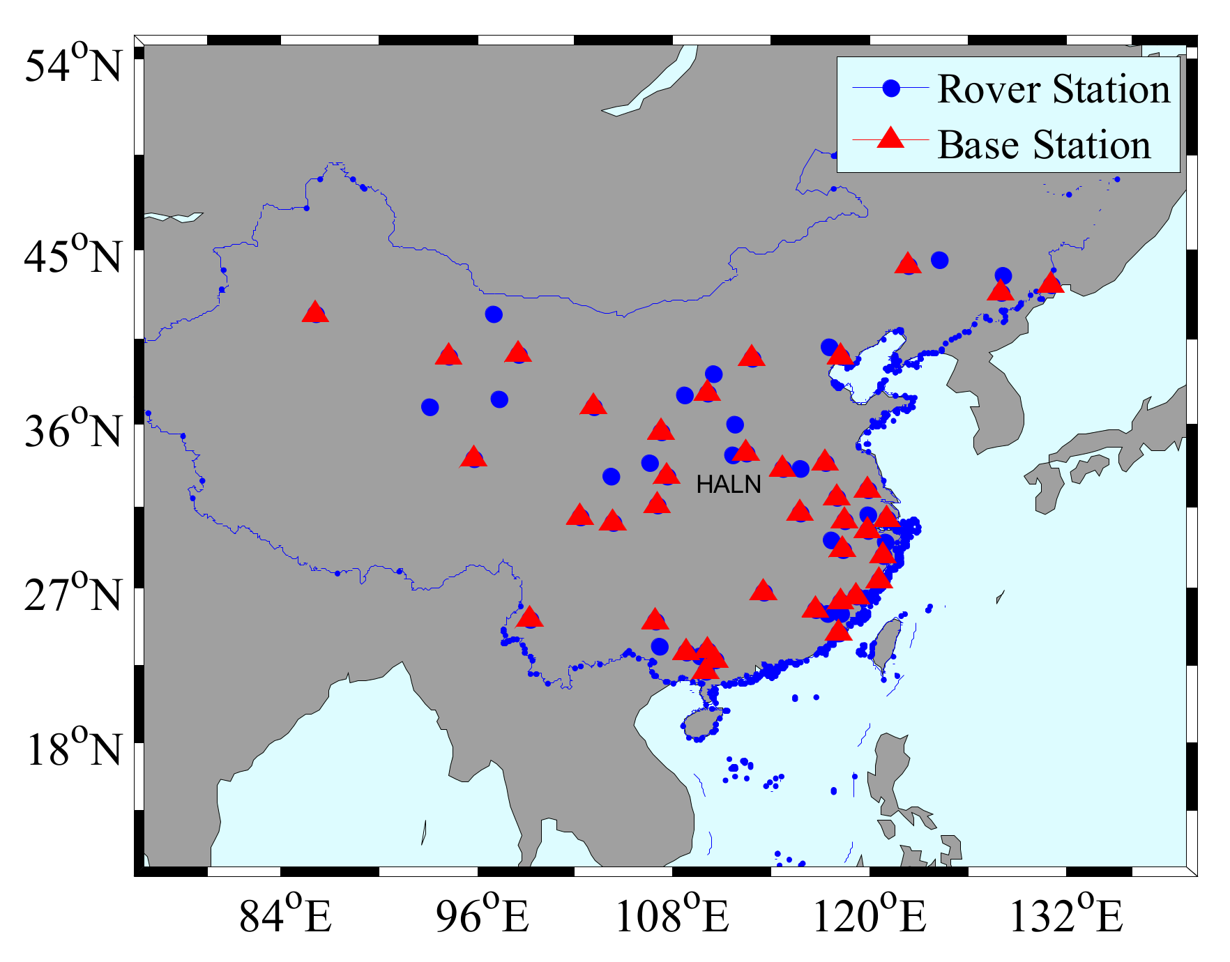
40] that was developed at Wuhan University was used in this study and the proposed strategy is thus implemented in PANDA. Observations collected with 60 stations on days of the year (DOYs) 74–80, 2015 were processed, where 40 stations were used as reference stations for the satellite clock and FCB estimation, and the remaining 20 stations were used as rover stations to perform the PPP ambiguity resolution.
Figure 1 shows the distribution of the stations used. The detailed processing strategies used for GPS + BDS FCB estimation and PPP ambiguity resolution are summarized in
Table 1.
To assess the benefits of ambiguity resolution when using GPS + BDS, we performed PPP ambiguity resolution for all 20 rover stations using data from a seven-day period. The daily observations were divided into 24 pieces composed of hourly sets; therefore, there were generally 168 hourly solutions for each station, which gave an overall total of 3360 solutions if there were no data losses. We assumed that the ambiguities could be fixed to the correct integers using the daily observations, and then the hourly ambiguities were compared with the daily “truth” to check its correctness. The WL ambiguity was fixed by rounding using a threshold of 0.25 cycles [
5,
6,
41]. Because of the strong correlation, the least-squares ambiguity decorrelation adjustment (LAMBDA) method was used to search the NL ambiguity, and a ratio test was used to validate the ambiguity resolution using a threshold of 2.0 [
14,
18]. The initial fixing time attained in each hourly session was recorded and analyzed and we then obtained the fixing percentages for different observation durations via calculation of the cumulative distribution of the initial fixing times.
5. Discussions
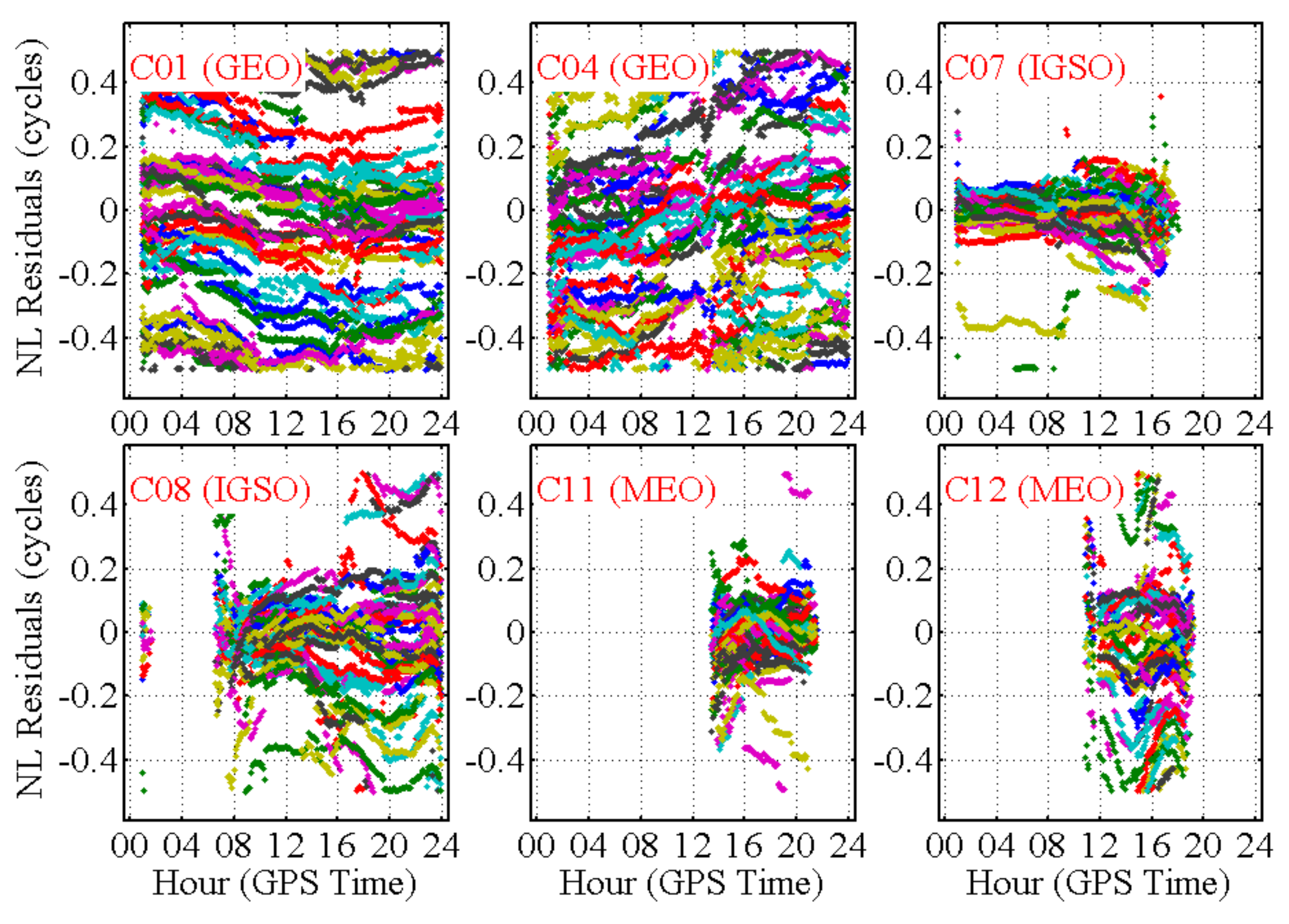
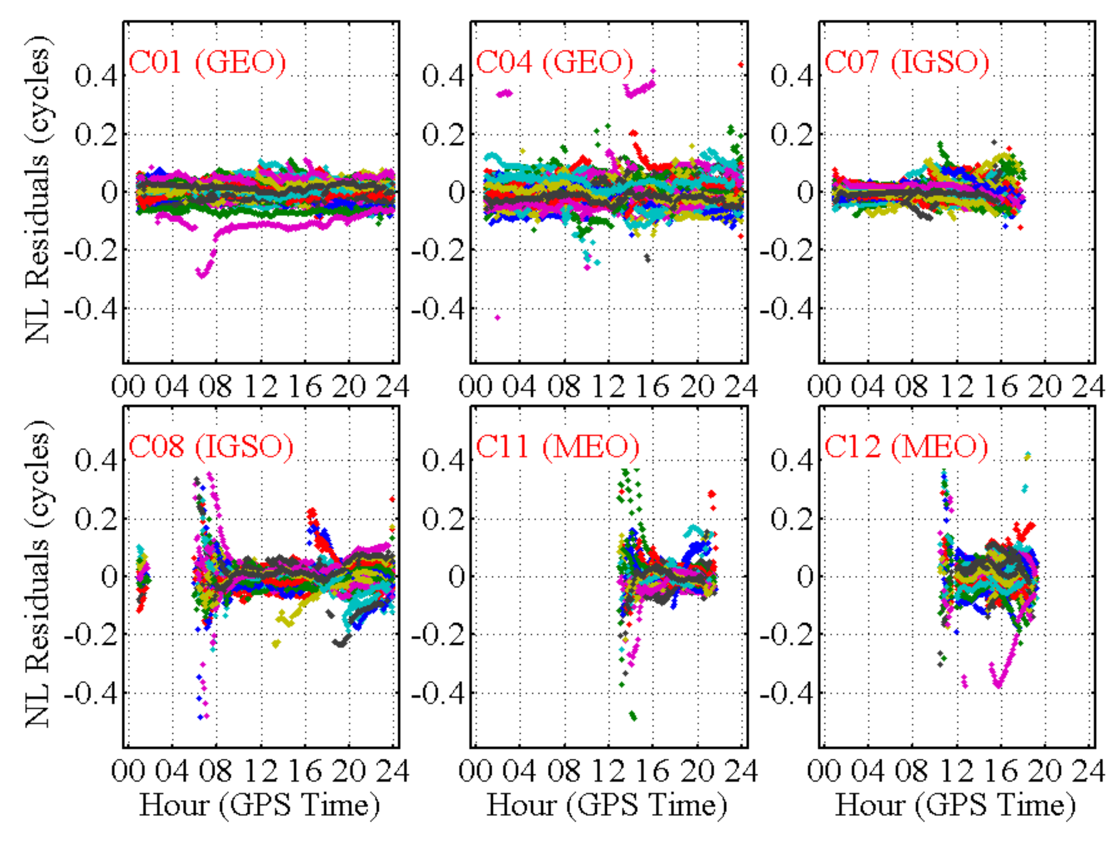
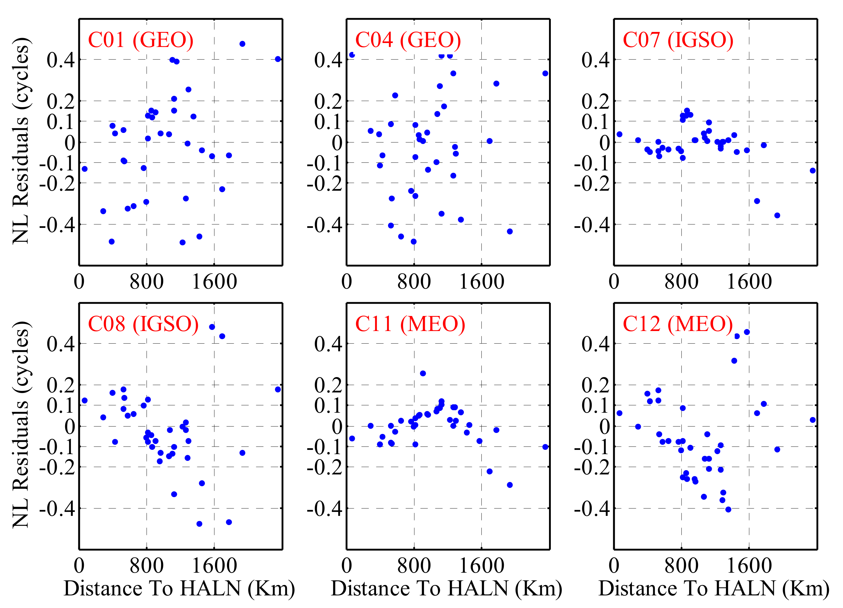
To provide further confirmation of the origins of the large residuals shown in
Figure 3, we selected the epoch in which the residuals were at their largest for each satellite and visualized the relationships between the NL residuals and the distance to the central station (HALN) as shown in
Figure 12. For C01 and C04, the epoch was 9:00:00; for C07, the epoch was 13:00:00; and for C08, the epoch was 20:00:00, while it was 16:00:00 for both C11 and C12. The figures show that for the GEO satellites, the NL residuals range between −0.5 and +0.5 and show no relationship to the distance to the central station. For the IGSO and MEO satellites, however, for which the NL residuals are not as large as those of the GEO satellites, the residuals gradually increase with increasing distance to the central station.
For comparison to
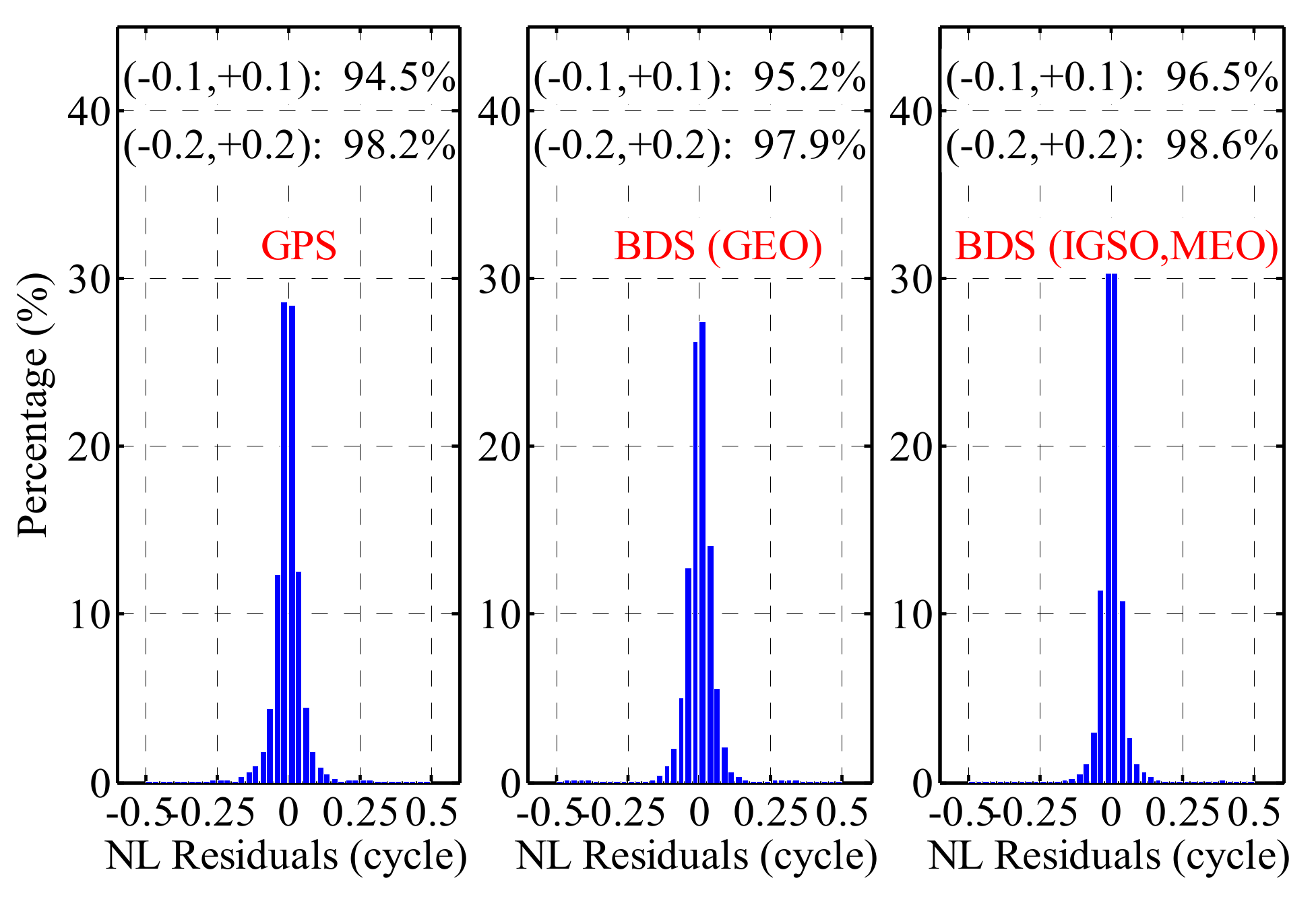
Figure 12,
Figure 13 gives the results when the orbit errors were considered. After consideration of the orbit errors, the residuals are all within 0.1 cycles for each satellite and for all stations, with the exception of three outliers. No trend between the size of the residual and the distance to the central station of the network is shown. Because the station-specific errors (i.e., troposphere errors and multipath errors) will not present such significant location-specific regulation (see
Figure 12) and because these errors will not disappear when the orbit errors are considered (see
Figure 13), it can thus be confirmed that the large residuals shown in
Figure 3 are caused by large orbit errors and the proposed method can thus work appropriately in eliminating the effects of large orbit errors on NL FCB estimation.
6. Conclusions and Outlook
With its five GEO, five IGSO and four MEO satellites, the BDS system plays an important role in PPP in the Asia-Pacific region. However, because of the lack of sufficiently well-distributed tracking stations and a poorly developed solar radiation pressure model, the orbit precision of the BDS satellites is low when compared with that of the GPS satellites [
24,
25,
27]; this is particularly true for the GEO satellites, which remain nearly stationary relative to the ground tracking stations. This poor orbit precision will affect the NL FCB estimation results of BDS satellites quite severely. This paper proposes a strategy for estimation of the GPS + BDS FCB based on consideration of the orbit error, and has demonstrated a GPS + BDS FCB estimation approach along with PPP ambiguity resolution in a simulated real-time model using the stations distributed across China.
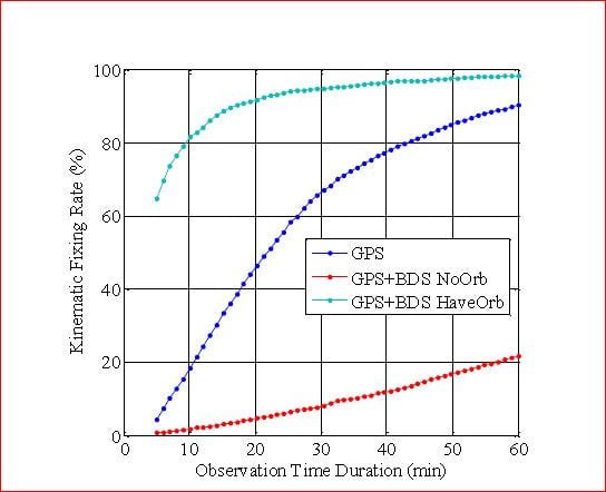
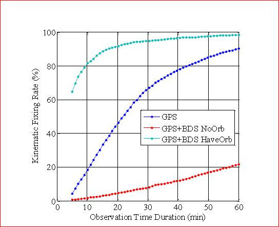
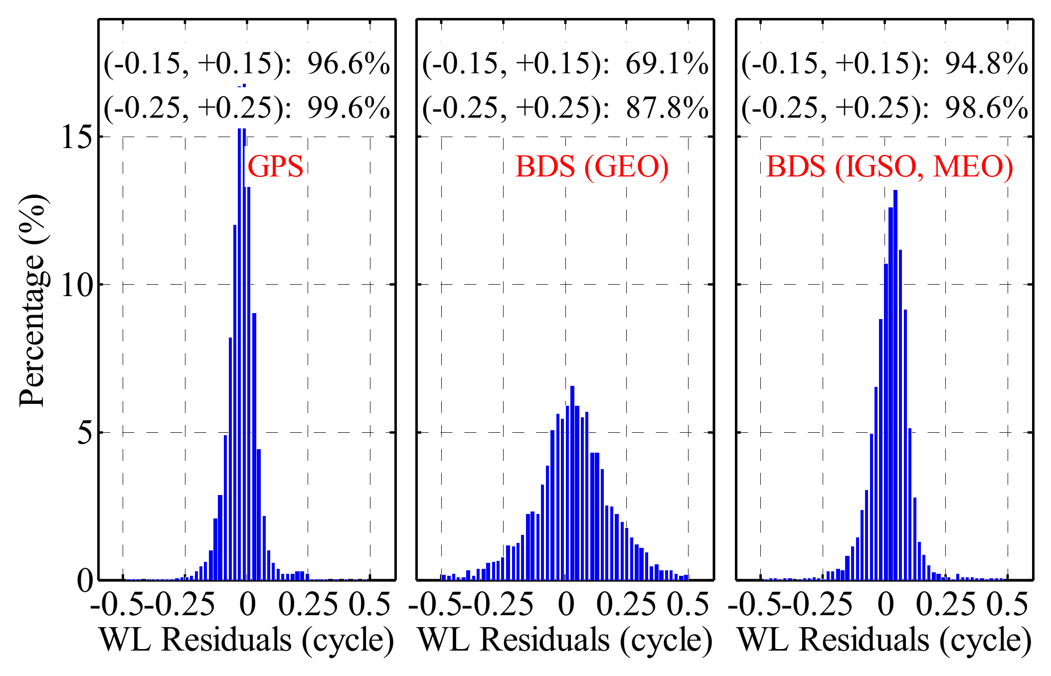
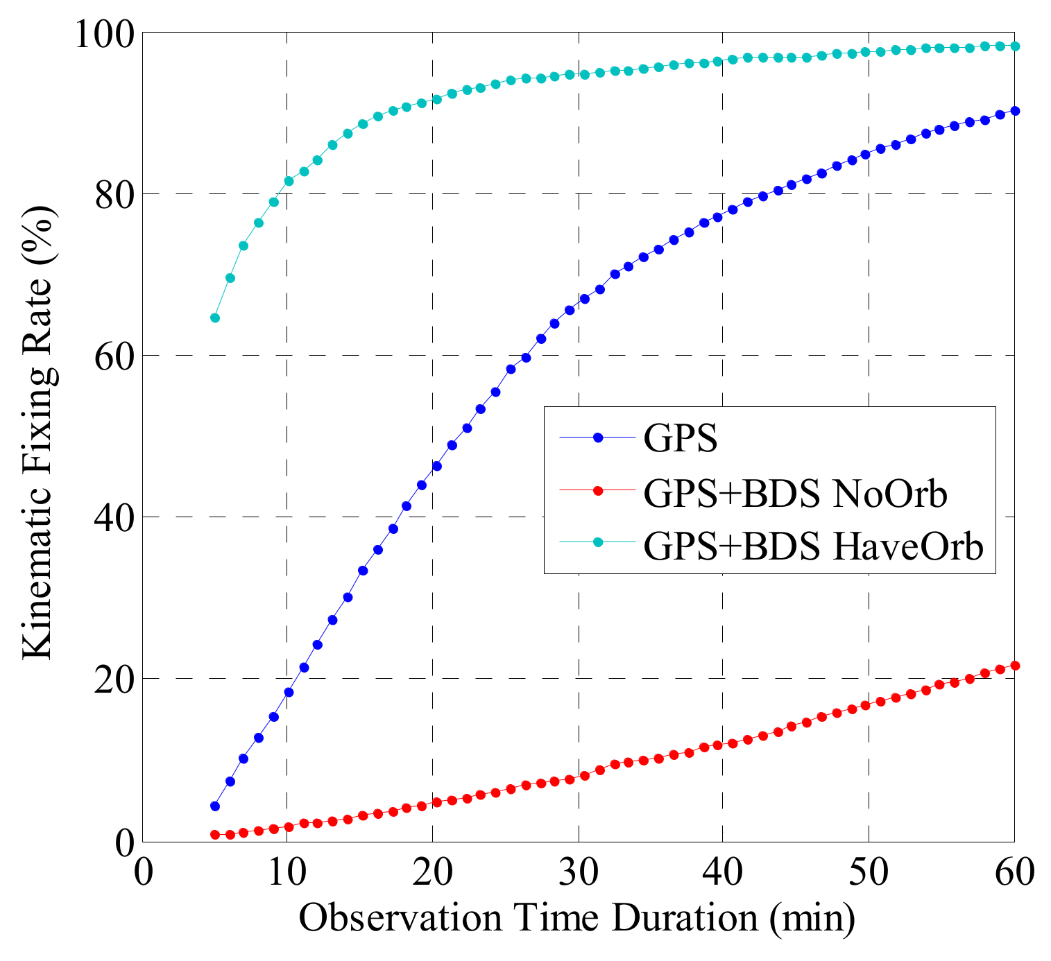
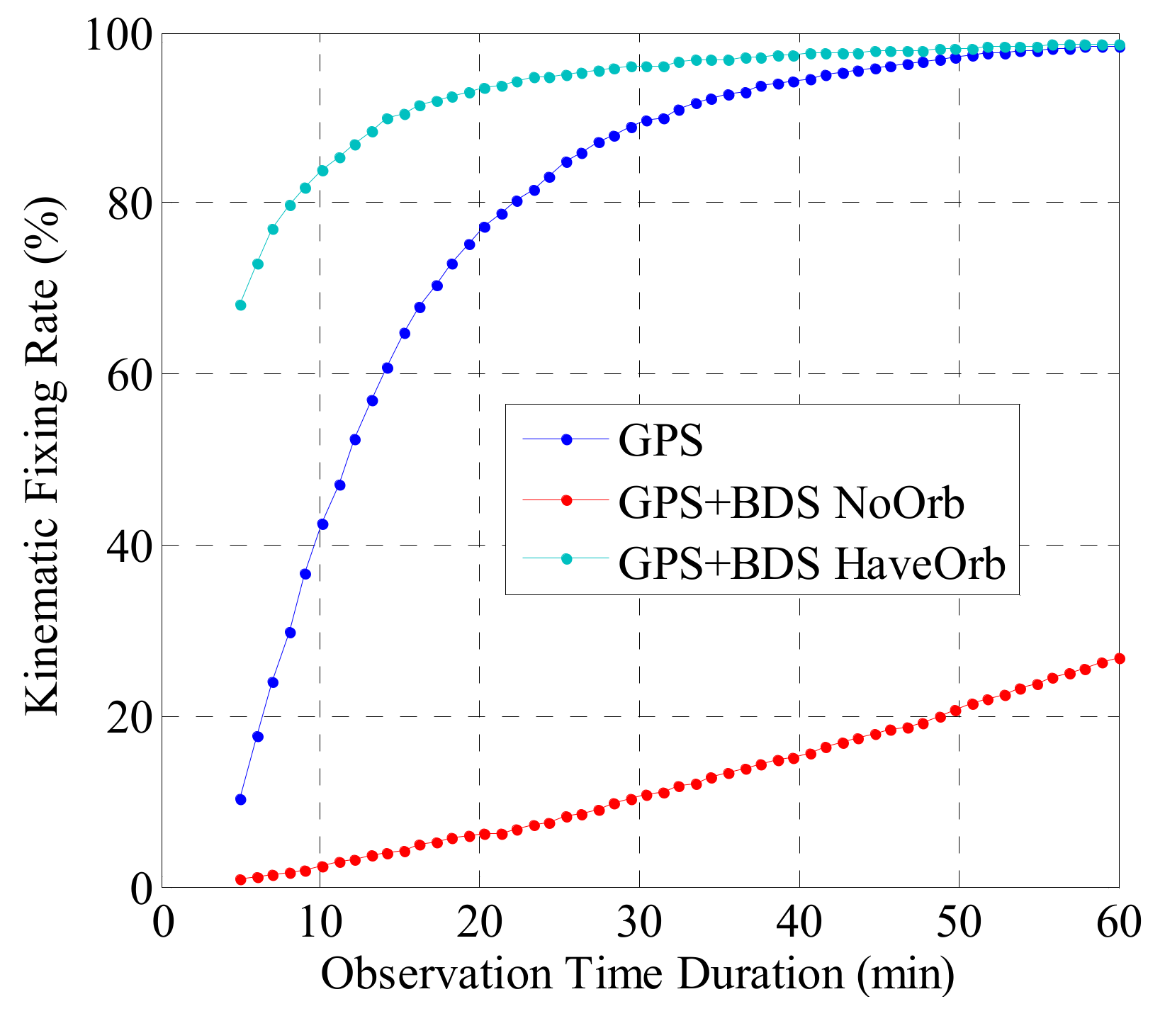
In general, more than 98% of the a posteriori residuals of the WL ambiguities are within cycles for the GPS, IGSO, and MEO satellites; while this figure falls to 87% for the GEO satellites. After the orbit errors were taken into consideration, more than 94% of the NL a posteriori residuals were within cycles for all satellite types. The contribution of the BDS observations to GPS-only PPP-IAR has also been investigated. In kinematic PPP, within a 5-min period, the fixing percentage for the solo GPS solution was only 4.27%; however, when the BDS was added, the percentage improved significantly to 64.56%. For observation periods of 10 min and 20 min, the fixing percentages were 18.33% and 46.25%, respectively, for the solo GPS, but rose to 81.53% and 91.73%, respectively, when using the GPS + BDS solution. With obvious contrast, if the GPS + BDS mode is used without consideration of the orbit errors, the fixing percentage only reaches 1.78% for a time period of 6 min and reaches 4.77% for both 10-min and 20-min observation periods. After the ambiguities are correctly fixed, the RMS position accuracy is degraded to 0.77, 0.67, and 2.88 cm for the north, east, and up directions, respectively, with improvements of 9.4%, 2.9%, and 2.0% when compared with the GPS-only solution.
Based on the scale factor, a wider tracking network distribution enables better orbit error estimation. The network used in this study covers an area with a radius of 1500 km, which is relatively small when compared with the globally distributed network of tracking stations. Therefore, with this network, we can only solve “part” of the orbit error, which may only satisfy the requirements for PPP-IAR within this network. Using greater numbers of Multi-GNSS Experiment (MGEX) stations [
43], we intend to investigate the performance of the proposed method over larger networks. In addition, the higher-order ionospheric delays and the bending effect both affect the PPP solutions [
44]. In this study, we have not considered the higher-order ionospheric delays as part of our PPP processing. Therefore, in future work, we will also consider these higher-order ionospheric delays and analyze their contributions to PPP-IAR performance.


