A Generalized Logistic-Gaussian-Complex Signal Model for the Restoration of Canopy SWIR Hyperspectral Reflectance

Abstract

The continuum of the SWIR (short-wave infrared) signals from 1320 to 1650 nm contains valuable information for effectively diagnosing water, chlorophyll, and nitrogen content. The SWIR spectra of in situ spectroradiometric data and airborne spectrometric images are frequently contaminated by significant noise. Based on a Logistic-Gaussian complex signal model (LGCM), the noise-free signals at 1330–1349 and 1411–1430 nm wavelengths can provide critical bases for restoring the 1350–1410 nm wavelength signals for a single point of data. This paper proposes a generalized LGCM (GLGCM) technique to expand the ability of LGCM to process large data with variant reflectance values. A 12-year-old red cypress plantation located in a central Taiwan temperate forest was selected for this study. Hundreds of reflectance spectra of tree crowns were obtained using an ASD FR Spectroradiometer. The in-laboratory blank test showed that the GLGCM technique was able to achieve sufficient performance with an RMSE (root mean square error) of 0.0015 ± 0.0005 and 0.0011 ± 0.0005 for the front-edge and end-edge signal bases respectively, and 0.0014 ± 0.0006 in between the two signal bases. A significant level of noise between −0.2 and 0.4 was successfully removed from the in situ contaminated reflectance in the 1350–1410 nm wavelengths. The estimation bias for the signals of front-edge and end-edge bases was low, averaging 0.0031 ± 0.0003 and 0.0032 ± 0.0012. The consistency between the blank test and the in situ experimental results indicates that the GLGCM technique has potential in using batch processing to fix the problem of the noisy SWIR spectra in spectroradiometeric data and also airborne spectrometric images.

1. Introduction

Hyperspectral spectroradiometers have been widely used for many years to collect pure reflectance of materials across multidisciplinary sciences such as geology, soil science, agriculture, and forestry. Reflectance of a variety of conifer and broadleaf species, grasses, crops, soils, and minerals have been collected by spectral libraries such as ASTER [1], SPECCHIO [2], SPECTATION [3], and VEGETATION [4] for extensive applications. Such hyperspectral surface reflectance provides references for environmental researchers to explore the sensitivity of a sensor’s spectral specification on signatures, target detection, and biophysical and biochemical research. Due to the spectral measurements being generally carried out in situ or in the laboratory by setting the sensor over a pure sample of the materials, the reflectance of any new material can expand the diversity of hyperspectral libraries and help environmental monitoring and management. The use of spectral libraries for example, involves identifying ingredients of compound feeding materials [5], soil-organic-carbon determination [6,7,8,9], urban material spectroscopy [10], coastal sediments [11], and coral reef health monitoring [12]. According to records of the Vegetation Spectral Library (VSL), more than 7200 users from 120 countries visited VSL during the period from December 2008 to March 2015 [13]. This indicates application of spectral libraries for environmental research and management has spread very rapidly over multidisciplinary sciences.

In forest remote sensing, spectral libraries of the crown of trees is considered to be more useful than that of leaves because they are generally collected in an area of decimeter or meter scale which is similar to a high spatial resolution airborne and satellite data. In other words, a tree crown reflectance is more appropriate to represent forest canopy spectra and provide support for the application of airborne or satellite image processing and analysis. As noted, many open-access hyperspectral reflectance libraries of trees have been developed via laboratory or field measurement using a portable spectroradiometer as well as airborne imaging spectrometers [14]. Although many spectral libraries contain data from temperate forests, it is imperative to develop ecosystem-based spectral libraries in order to expand their usability and applications in tropical/sub-tropical forests.

It is well known that the vegetation spectra measured in the field are frequently noisy in the region of shortwave infrared (1000–2500 nm). This problem is particularly pronounced in 1350–1410 nm and 1700–1900 nm because of the broad absorption of atmospheric water vapor [15], thus these spectra are rarely used in practical sensing [16,17,18,19,20]. Even though the low signal-to-noise ratio (SNR) is considered as troublesome, the absorption feature centered at 1450 nm and 1940 nm has been demonstrated as quite valuable for estimating the water content of plants [21,22,23,24] and nitrogen content [25,26,27]. In general, a degraded hyperspectral is represented as a combination of a true signal and additive noise and a denoising method is designed to estimate the original signal by penalized least squares optimization [28]. In articles, a variety of modern denoising algorithms have demonstrated their excellence in dealing with contaminated images such as block-matching 3D-transform shrinkage (BM3D) [29], K-SVD [30], independent component analysis (ICA) [31] and wavelet transform and ICA-based fusion method (WT-ICA) [32]. More recently, the low-rank based approaches such as low-rank matrix recovery (LRMR) and noise-adjusted iterative low-rank matrix approximation (NAILRMA), in dealing with the sparse noise in hyperspectral data, were suggested for preprocessing of hyperspectral data due to their capability of improving the accuracy of vegetation classification [28]. These methods work at the sites of the contaminated bands from the spatial and/or transform domain. As noted, the AVIRIS image provides 224-bands hyperspectral data covering the 400–2500 nm spectral range and is known for its high signal-to-noise ratio for retrieving parameters of forest canopy [33]. However, the noisy SWIR (short-wave infrared) bands were always removed from the images before early 2010 and alternatively the reflectance of the noisy bands was directly replaced with an estimate of a simple linear model in the latest version of the USGS Spectral Library published in 2017 [14]. The atmospheric water-vapor absorption causing noise in the SWIR region is extremely large, it does not logically belong to any one of the four noise assumptions, i.e., signal independent noise, signal dependent noise, sparse noise, and pattern noise proposed in [28] and the denoising cannot be done in the absence of such noisy bands.

A linear model can be used to roughly redraw the missed reflectance of the particular SWIR wavelengths for the AVIRIS image, it is still unable to provide spectral information of the SWIR continuum of trees because it behaves nonlinearly and changes substantially as a function of physiological stress [24]. The ability to retrieve vegetation water content or water thickness using hyperspectral data is of particular importance to forest security in that it can provide a way of estimating live fuel water content to facilitate the consideration of fire risk over a forest area [34,35].

In contrast to the denoising methods mentioned earlier, the estimation of the signal of SWIR bands using simple linear model is called signal restoration. Considering that the VNIR–SWIR reflectance curve of green leaves raises as water content decreases [36] and reflectance of any materials appear to vary slightly in natural status, the use of a single band reflectance based indicator for live fuel water content estimation may be affected by the variation of pixel value. In contrast, the continuous spectra of the 1450 nm absorption region can substantially provide reliable information of water content and can even detect the water stress in tree leaves [24]. So, restoring the shortwave infrared signal will make such continuous spectra available for field-measured data and therefore is definitively able to be of benefit in vegetation monitoring. In contrast to the post processing of median filter [37], the technique of logistic-Gaussian complex signal model (LGCM) has been demonstrated as efficient in restoring the crucial signals of the noisy shortwave infrared region from 1350 to 1410 nm [24].

Unfortunately, the prototype of the LGCM technique was designed to only process single vegetation spectra. In field spectral experiments, the spectral information of tree crowns are generally collected via multiple spectral measurements. Trees under direct light or shading area will have a reflectance that will show a quite different level along the spectra. The difference of their reflectance will be significant for the two particular wavelengths at the two ends of the noisy SWIR region. Obviously, restoration of the SWIR signals is always necessary for a large number of spectral measurements but applying the LGCM to process data to each individual measurement separately will become time consuming and troublesome. In other words, the prototypical LGCM method will be inefficient and not practical for mass data processing. This is particularly evident for the processing of airborne hyperspectral images, such as AVIRIS, in which a huge number of vegetation pixels is supposed to need an appropriate generalized LGCM method for automatic processing. Therefore, the objectives of this study were to (1) propose a protocol for deriving the generalized parameters of the logistic-Gaussian complex signal model using multiple regression analysis; and (2) examine the appropriateness of the generalized Logistic-Gaussian complex signal model (GLGCM) in restoring the signal of the noisy shortwave infrared spectra. The sensitivity of the GLGCM technique on the sources of noise-free signal was also addressed.

2. Materials and Methods

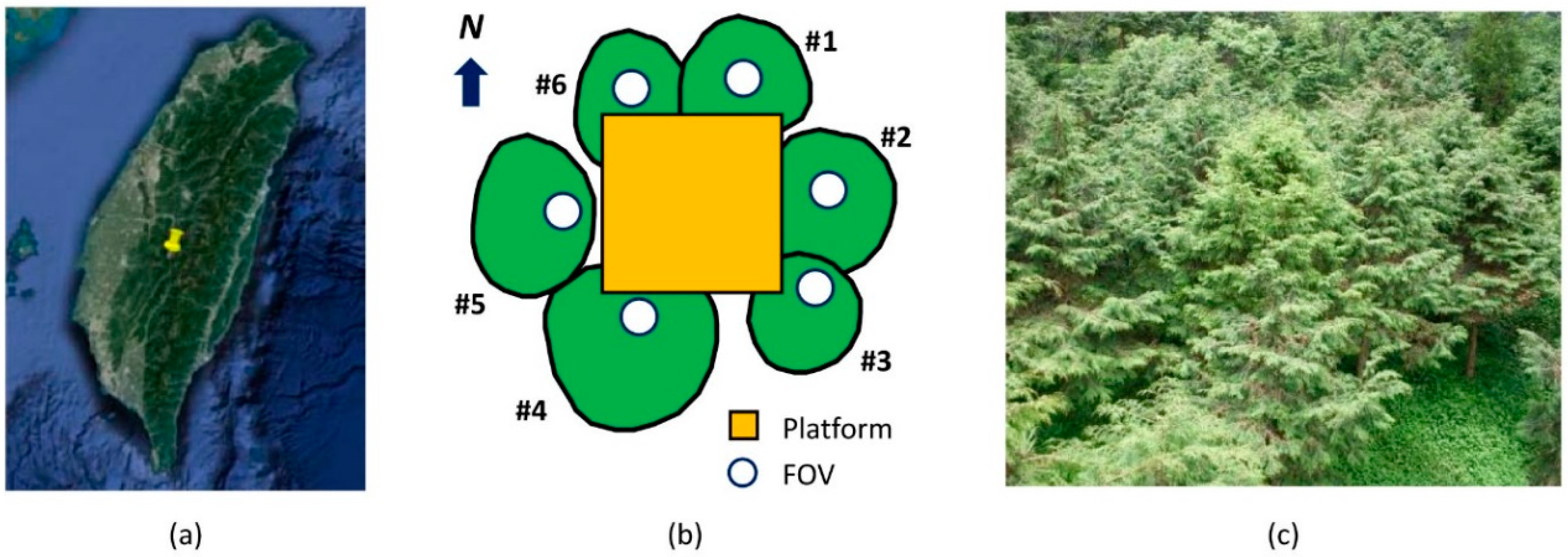
2.1. Study Site and Data Collection

A red cypress (Chamaecyparis formosensis Obtusa) plantation located on the Alishan Mountain in central Taiwan (Figure 1) was selected for this study. The tree species is endemic to the temperate forest of the island and distributed over a wide range of altitudes from 1000 to 2800 m. The elevation of the study site was around 2267 m. Meteorological records showed that the mean annual temperature and rainfall was 10.6 °C and 4000 mm respectively, and the relative humidity varied between 65% and 88%.

Figure 1b shows the experimental design of a 6.5-m-height watchtower located at the center of a group of trees for collecting in situ red cypress spectra. The six red cypresses were 12-years old and with heights around 4–5 m. Spectral measurements were carried out on the platform at the local time of 9:20–10:00 a.m. from October 2008 to September 2009. An ASD FR spectroradiometer was deployed using a 25° field-of-view fiber optic cable at approximately 2.25 m above the tree crown. The measurements were made in the order of the reference Spectralon and the target tree iteratively to collect 5-paired replications for a single tree. During the measurements, a dark current measurement was periodically taken to calibrate the signal of the VNIR detector every 20 min. A reflectance was determined by dividing the reflected target radiance by the irradiance of the reference Spectralon. In total 306 pairs of field spectral measurements were observed. The field data were randomly divided into two subsets for training and assessment which contained 70% and 30% of the observations respectively. Additionally, foliage samples of the red cypresses were collected for in-laboratory spectral measurements under artificially controlled light environments using an artificial illuminator (USHIO jc 14.5 V–50 WC, manufactured by Ushio America, INC., Cypress, CA, USA). As a result, 30 in-laboratory red cypress spectra were used to examine the appropriateness of the algorithm protocol for this study.

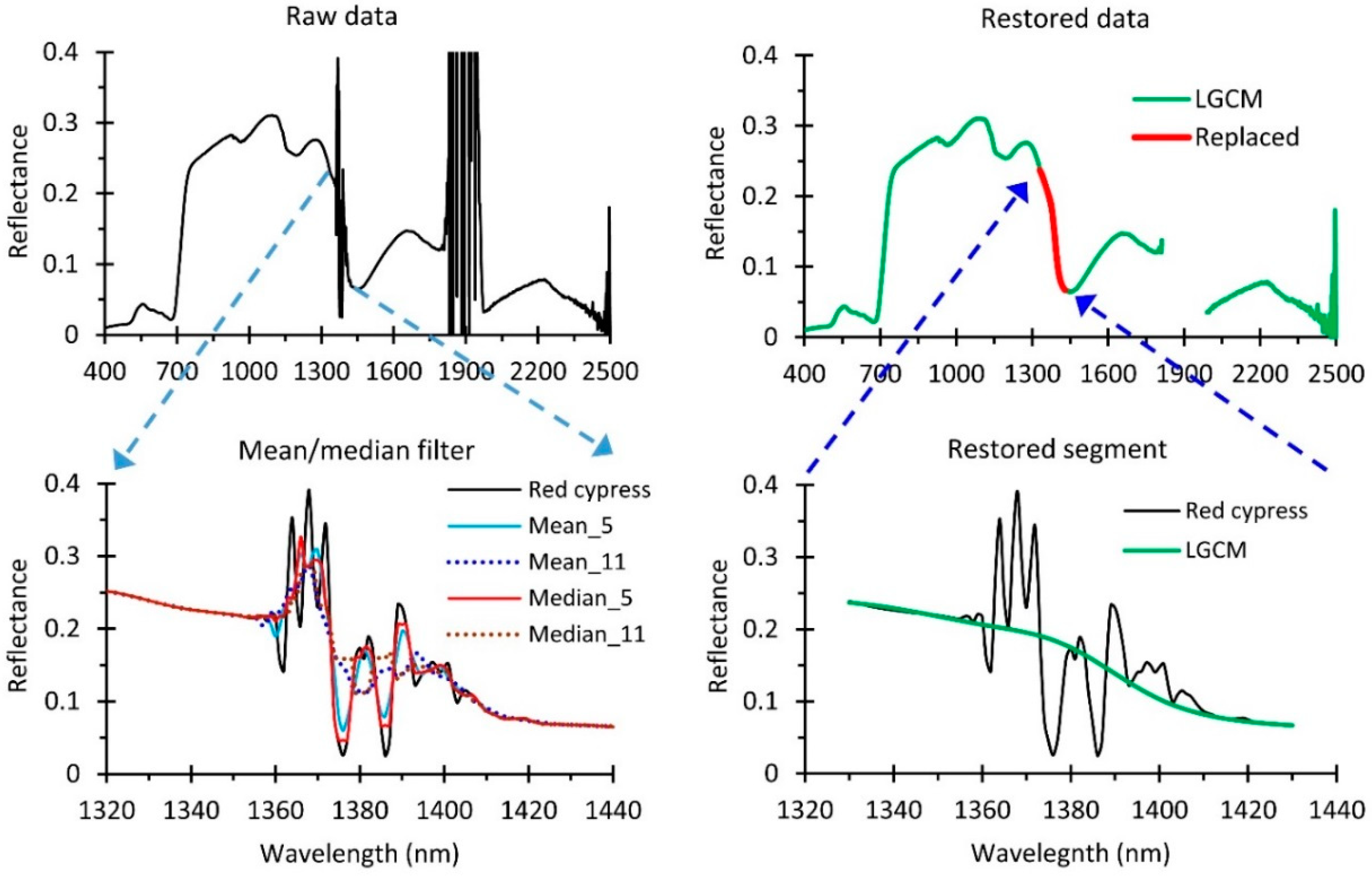
2.2. The Prototype of the Logistic-Gaussian Complex Signal Modelling (LGCM) Technique

In general, the noise in the SWIR regions at the specific wavelengths 1350–1410 nm and 1770–2000 nm was extremely sharp. As shown in Figure 2, the reflectance curve (the black curve in the upper left subfigure) measured in-situ from the tree crown of a red cypress was obviously contaminated due to the water vapor absorption, low signal-to-noise ratio in the SWIR regions [38] and the high humidity of the atmosphere [24]. A moving average or median filtering method was not able to fix this problem (the blue and red lines in the lower right subfigure). The complicated vegetation spectra in the region from 1770–2000 nm appeared as a pattern with changing curve behavior. Fortunately, the noise-free vegetation reflectance in the region from 1300 to 1440 nm was found to be a typical S-type curve that provided the possibility of restoring the signals at the 1350–1410 nm wavelengths [24]. This is of particular benefit in enabling the use of valuable SWIR spectra of the water absorption region to explore the water stress and even the chlorophyll content of tree crowns. The technique of the Logistic-Gaussian complex signal model (LGCM) was developed based on medical replacement surgery. A signal segment for the particular wavelengths was first restored using the LGCM model (lower right subfigure in Figure 2); the originally noisy segment was then removed and replaced with the restored signal segment (upper right subfigure in Figure 2).

Mathematically, the original LGCM technique retrieves a primary signal (pR_λ) and a secondary signal (rR_λ) using Equations (1) and (2) respectively for each wavelength λ in the region of 1350–1410 nm (hereafter “the SWIR”). The retrieved values at each λ (in nanometer) are then added up to determine the restored reflectance R_λ (Equation (3)). Typically, the reflectance curve of trees in the noisy SWIR region, declines from the shorter towards the longer wavelength. The parameters max and min of the four-parameter logistic sub-model (Equation (1)) stand for the reflectance of the point at the front-edge (on shorter wavelength side) and end-edge (on longer wavelength side) signal bases. EC50 identifies the inflection point or the midpoint of the curve between the two particular wavelengths of max and min. Hillslope describes the curve’s slope at its midpoint, the larger the Hillslope value the greater the slope. The rR_λ acts like a bell-shape curve which is generally concentrated at the center wavelength of the noisy SWIR region and decreases on either side. The parameters a and b in Equation (2) describe the level of Gaussian peak that locates at the center position (λ₀) of the SWIR region and the width of the bell respectively.

$$p{R}_{\lambda }=MIN+\left(MAX-MIN\right)\left[1+{\left(\lambda /E{C}_{50}\right)}^{Hillslope}\right]$$

(1)

$$r{R}_{\lambda }=a·EXP\left\{-0.5{\left[\left(\lambda -{\lambda }_0\right)/b\right]}^2\right\}$$

(2)

$$\mathit{restored}\text{\_}{R}_{\lambda }=p{R}_{\lambda }+r{R}_{\lambda }$$

(3)

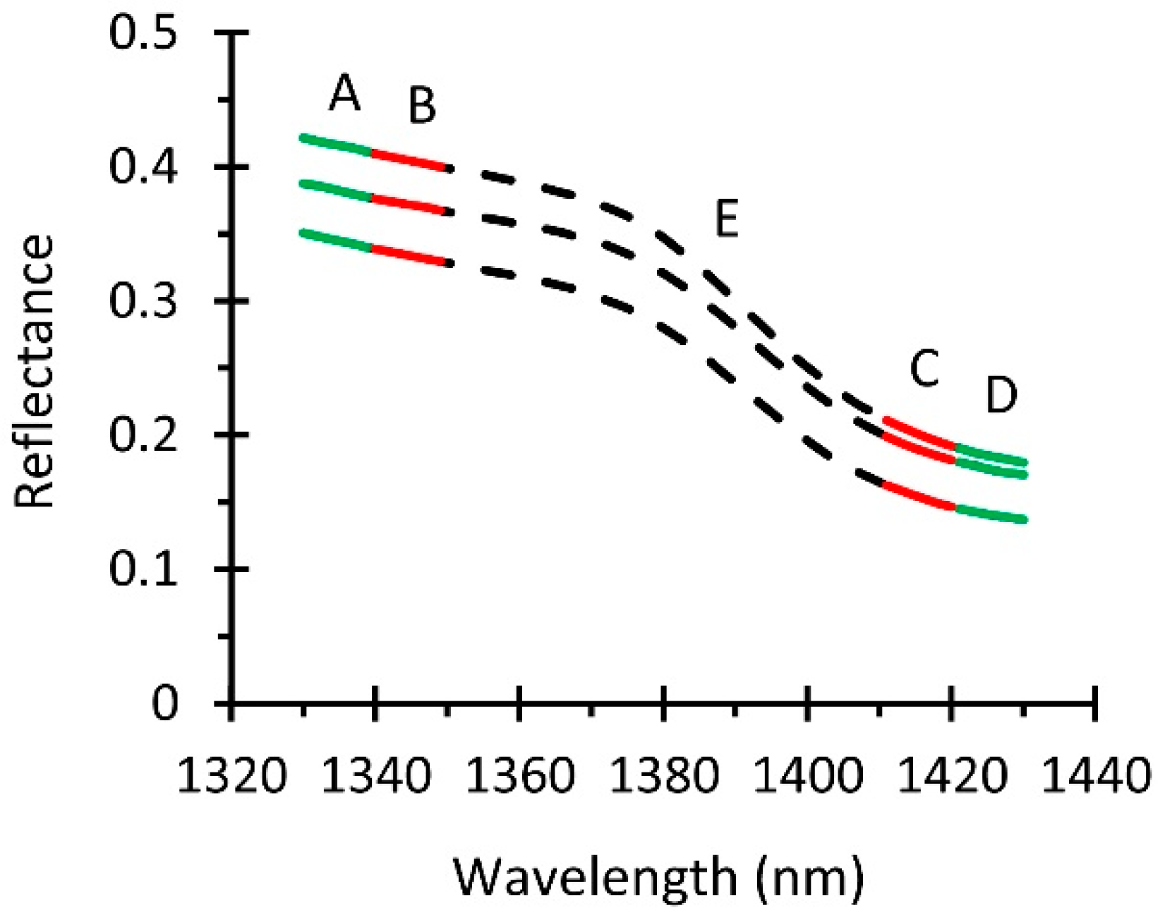
2.3. Deriving Parameters of a Generalized Logistic-Gaussian Complex Signal Model

In practice, the reflectance curve of tree crowns reveals a typical pattern over the whole region from visible to short-wave infrared. The curve will level up or level down due to the changes of light environment as well as the water and chlorophyll contents. In contrast to the typical pattern in the whole region, the segmented curve of the SWIR also behaves in a notably similar way. As shown in Figure 3, the SWIR reflectance curve of red cypress jumped up/down to a different degree among the examples. Such jumps at both sides appeared unbalanced. Therefore, the critical point of developing a generalized LGCM (GLGCM) technique is to enable the original LGCM model to be flexible and adjustable to fit variant signals of the two bases, i.e., the noise-free signals at the subparts of A–D in Figure 3. In other words, the proposed algorithm serves to harmonize the parameters of the original LGCM model with the signals at A–D bases. To meet this requirement, a multiple linear regression method was applied to derive the estimates of the MAX, MIN, EC50, and Hillslope that were used to construct the prototypical logistic and Gaussian sub-models (Equations (1) and (2)) to determine the primary signal and the estimates of the a, b, and λ₀ for retrieving the compensatory or secondary signal.

The bands of hyperspectral data are highly correlated. In order to avoid causing serious problems due to multicollinearity, the redundant signals in each subparts of the SWIR segment were simply generalized by an averaging method instead of using all signals for regression analysis. Thus, a representative signal of the noise-free signals at each subpart of the SWIR segment in Figure 3 was firstly determined as the reflectance average of that subpart spectra. Specifically, the ${\overline{\rho }}_A$, ${\overline{\rho }}_B$, ${\overline{\rho }}_C$, and ${\overline{\rho }}_D$ stand for the reflectance average of the 1330–1339, 1340–1349, 1411–1420, and 1421–1430 nm respectively.

Let the representative signals of the four subparts as the independent variables, and the particular parameters of the primary signal model or the secondary signal model be the dependent variables, then a multiple linear regression model in the form of Equation (4) or (5) is derived as the generalized parameter of the MIN/MAX and the EC50/Hillslope respectively which were labelled GMIN, GMAX, GEC50, and GHillslope to differentiate them from the original prototypical form. Additionally, Equation (6) is derived for the generalized parameters Ga, Gb, and Gλ₀ of the prototypical parameters a, b, and λ₀ of the secondary signal model. Finally, a signal of the SWIR restored by the GLGCM model is determined as the combination of the two estimates obtained by Equations (7) and (8).

The performance of the GLGCM method in deriving the SWIR spectra was evaluated using the accuracy measure RMSE, i.e., the root mean square error [39]. The measure was calculated based on the bias of the front-edge signal base (1030–1049 nm), end-edge signal base (1411–1430 nm), and the central segment or in-between the signal bases (1050–1410 nm) where the physical meaning of this measure is the average bias of reflectance per unit wavelength, nm.

$$Y={\beta }_0+{\beta }_1{\overline{\rho }}_A+{\beta }_2{\overline{\rho }}_D$$

(4)

$$Y={\beta }_0+{\beta }_1{\overline{\rho }}_A+{\beta }_2{\overline{\rho }}_B+{\beta }_3{\overline{\rho }}_C+{\beta }_4{\overline{\rho }}_D$$

(5)

$$Y={\beta }_0+{\beta }_1{\overline{\rho }}_B+{\beta }_2{\overline{\rho }}_C$$

(6)

$$p{R}_{\lambda }=GMIN+\left(GMAX-GMIN\right)\left[1+{\left(\lambda /GE{C}_{50}\right)}^{GHillslope}\right]$$

(7)

$$r{R}_{\lambda }=Ga·EXP\left\{-0.5{\left[\left(\lambda -G{\lambda }_0\right)/Gb\right]}^2\right\}$$

(8)

3. Results and Discussion

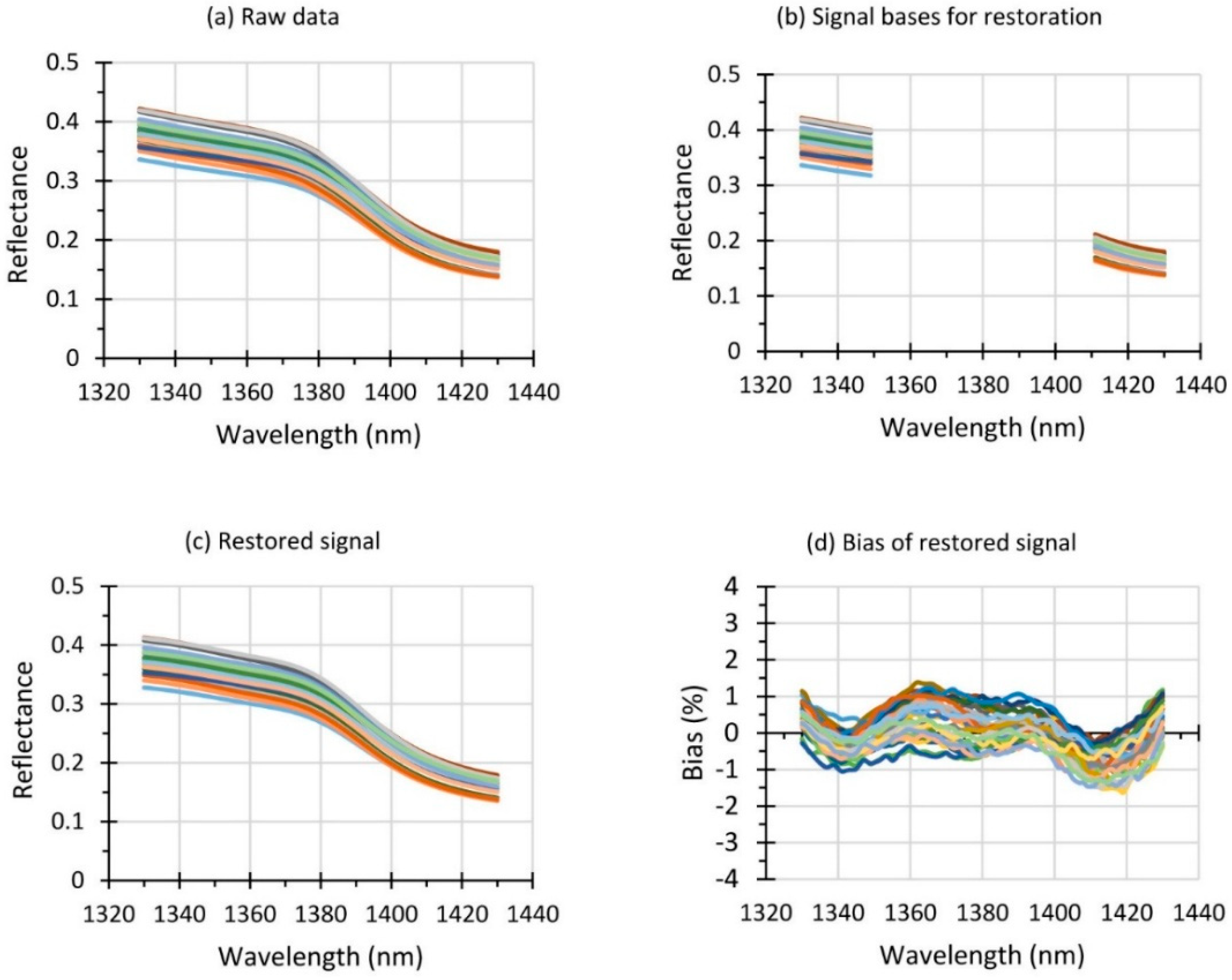
3.1. A Blank Test of the Performance of the GLGCM Technique in Restoring the SWIR Signals

Noise-free samples of red cypress reflectance were collected using laboratory based spectral experiments. As shown in Figure 4a, the segments of the SWIR spectra were used to carry out a blank test for examining the performance of the GLGCM technique in restoring the signal of the SWIR. The regression model for each of the generalized parameters of the logistic simplex signal model as well as the Gaussian simplex signal model are summarized and listed in

Table 1. Summary of the laboratory based data for generalized Logistic-Gaussian complex signal model (GLGCM) logistic and Gaussian sub-models.

Models	Parameters	Equations	R2
Logistic sub-model	GMax	$GMAX=0.00807+1.0741{\overline{\rho }}_A-0.1229{\overline{\rho }}_D$	0.99
	GMin	$GMIN=0.00757-0.0970{\overline{\rho }}_A+1.0070{\overline{\rho }}_D$	0.99
	GEC50	$GEC50=1385.18-803.6{\overline{\rho }}_A+765.0{\overline{\rho }}_B+980.3{\overline{\rho }}_C-939.8{\overline{\rho }}_D$	0.98
	GHillslope	$GHillslope=77.67-2935{\overline{\rho }}_A+3234{\overline{\rho }}_B-1869{\overline{\rho }}_C+1557{\overline{\rho }}_D$	0.96
Gaussian sub-model	Ga	$Ga=0.004636+0.1843{\overline{\rho }}_B-0.2263{\overline{\rho }}_C$	0.91
	Gb	$Gb=13.1198-1.2090{\overline{\rho }}_B+2.1230{\overline{\rho }}_C$	0.04
	$G{\lambda }_0$	$G{\lambda }_0=1378.91-7.71{\overline{\rho }}_B+19.79{\overline{\rho }}_C$	0.24

. The results showed that the value of a generalized MAX/MIN/EC50/Hillslope for all SWIR spectra can be precisely estimated. Specifically, 99% of MAX/MIN variations for all the sample spectra can be explained by the GMAX/GMIN parameter using the representative signals ${\overline{\rho }}_A$ and ${\overline{\rho }}_D$, and the derived GEC50/GHillslope was able to explain more than 96% of EC50/Hillslope variations using ${\overline{\rho }}_A$, ${\overline{\rho }}_B$, ${\overline{\rho }}_C$, and ${\overline{\rho }}_D$. In contrast to the high performance of the generalized logistic sub-models, the generalized Gaussian sub-models parameters Ga/Gb/Gλ₀ achieved an ability of 91%/4%/24% in explaining the variation of a/b/λ₀ using ${\overline{\rho }}_B$ and ${\overline{\rho }}_C$. The results indicated that the secondary signal is primarily related to the Gaussian peak parameter “a” while the Gaussian width parameter “b” and location parameter “λ₀” contribute insignificantly as the primary signal was determined a priori. In other words, applying the GLGCM technique to restore the SWIR signals can be first carried out using a crucial generalized logistic sub-model and followed with a generalized Gaussian sub-model, in which the Ga appears to be critical for making a better estimation of the secondary signals while both Gb and Gλ₀ seem not to be critical and may be replaced by “a” and “b” of any one of the samples. The central segment of the blank-test spectra was intentionally missed and only the signal bases of the spectra shown in Figure 4b were used to restore the missed spectra using the generalized logistic primary signal sub-model and the generalized Gaussian secondary signal sub-model. As shown in Figure 4c,d, the segment of the continuous spectral curve of such restored SWIR signals showed a high similarity to the in-laboratory SWIR spectra with a bias less than 2% of the original reflectance at each wavelength. Briefly summarized, the results showed an average RMSE per nanometer reflectance of 0.0015 ± 0.0005 for the front-edge base (the wavelength from A to B), 0.0011 ± 0.0005 for the end-edge base (the wavelength from C to D), and 0.0014 ± 0.0006 in between the two bases (the wavelength from B to C, the central segment E). This demonstrated that the GLGCM algorithm produces reasonable results and is also promising in restoring plant reflectance at the 1350–1410 nm wavelengths.

3.2. Sensitivity of the Generalized Parameters of Logistic Primary Signal and Gaussian Secondary Signal Sub-Models

With the laboratory based reflectance of the SWIR segment being known, a sensitivity analysis of the GLGCM technique can be made by changing the source of the generalized parameters in the logistic primary signal sub-model and the Gaussian secondary signal sub-model. As shown in Table 1, all the generalized parameters of the prototypical GLGCM were estimated using a multiple regression method and the representative signals of the bases A–D. A different GLGCM structure can instead be formulated if the GMAX/GMIN is derived using one or two bases of the SWIR signals or due to the GEC50/GHillslope and/or the Ga/Gb/Gλ₀ obtained via the published literature [24].

Based on the same scale of reflectance (0–1) in the raw data, the performance of GLGCM was compared from the points of front-edge, end-edge, and in-between subparts. The prototypical GLGCM method (structure 1) was able to achieve a reflectance bias of RMSE = 0.0014 in the segments between the front-edge and the end-edge bases, the best accuracy among the variant structures (

Table 2. The ways or sources of the generalized parameters of GLGCM sub-models.

Structure	GMAX	GMIN	EC50/GHillslope	Ga	Gb	Gλ0
1	A and D	A and D	A, B, C, and D	B and C	B and C	B and C
2	A and D	A and D	A, B, C, and D	B and C	x #	x
3	A and D	A and D	A, B, C, and D	x	x	x
4	A and D	A and D	x	B and C	B and C	B and C
5	A	D	A, B, C, and D	B and C	B and C	B and C
6	A	D	A, B, C, and D	x	x	x
7	A	D	x	B and C	B and C	B and C
8	A	D	x	x	x	x

^# The code “x” indicates the particular parameter published in [24].

). When the Gb and Gλ₀ parameters were replaced by the coefficients published in [24] (structure 2), the RMSE was almost equal to structure 1, indicating that such parameters have quite minor significance. This is almost identical to the model R² shown in Table 1. Figure 5a,b also showed that the bias percentage ($\mathrm{bias}\%=\left(\rho -\widehat{\rho }\right)/\rho \times 100$) of every single nanometer-scale signal was mostly between −1% and +1%. As the Ga was also replaced by a published coefficient (structure 3), the RMSE was almost doubled but still could be considered as low level. The increment of RMSE mainly occurred at the central wavelength of the segment (Figure 5c).

When the GMAX and GMIN was derived using only the representative signals of the base segment next to it such as A or D (structure 5), the bias of such restored signals for the segment between the two bases became three times larger than structure 1 (

Table 3. Comparisons of the performance (mean ± standard deviation of the root mean square error (RMSE)) of the GLGCM technique with a variety of parameter sources using the laboratory based data.

Segments	Structure 1	Structure 2	Structure 3	Structure 4	Structure 5	Structure 6	Structure 7	Structure 8
Front-edge (A–B)	0.0015 ± 0.0005	0.0015 ± 0.0005	0.0015 ± 0.0005	0.0050 ± 0.0009	0.0058 ± 0.0014	0.0058 ± 0.0015	0.0108 ± 0.0008	0.0108 ± 0.0009
End-edge (C–D)	0.0011 ± 0.0005	0.0010 ± 0.0005	0.0011 ± 0.0005	0.0187 ± 0.0016	0.0013 ± 0.0008	0.0013 ± 0.0008	0.0191 ± 0.0014	0.0192 ± 0.0014
Central (E)	0.0014 ± 0.0006	0.0015 ± 0.0007	0.0026 ± 0.0012	0.0309 ± 0.0031	0.0045 ± 0.0013	0.0034 ± 0.0013	0.0335 ± 0.0026	0.0315 ± 0.0033

). Although the increase of estimation bias was still quite small and could probably be acceptable, the pattern of such bias seemed to disperse more significantly in the SWIR segment. As can be seen in Figure 5e, the bias percentage was enlarged up to 5% (from +3% on the left to the −2% on the right base). This situation was similar to the cases of structure 6 (Figure 5f) vs. structure 3 (Figure 5c) and the results indicated that the ability of both A and D bases in regulating a reasonable estimation of GMAX and GMIN parameters will be inconsistent or unbalanced and consequently a larger/smaller bias% on the front-edge/end-edge base can be induced.

The appropriateness of utilizing GEC50 and GHillslope is confirmed by the provision of the additional critical point that enables the GLGCM technique to achieve excellent performance in restoring the SWIR signals. In contrast to Figure 5a, structure 4 applied the original parameter of EC50 and Hillslope published in [24] instead of the GCE50 and GHillslope for estimating the primary signal and with the Ga, Gb, and Gλ₀ for estimating the secondary signal. An extremely large bias% was found in the region from 1340 to 1430 nm (Figure 5d), and the average RMSE per nanometer was 0.0050/0.0187/0.0309 for the front-edge/end-edge/central segment of the SWIR (Table 3). Particularly, the RMSE in the end-edge/central segment was almost 17/22 times larger than the one of structure 1. Comparison with the RMSE (Table 3) and the bias% of structures 7 and 8 shown in Figure 5g,h indicates that the effects of changing the parameters GMAX and GMIN as well as the Ga/Gb/Gλ₀ were not significant. It was therefore concluded that the GEC50 and GHillslope as well as the GMAX and GMIN are the major factors controlling the overall performance of the GLGCM technique.

3.3. Field Based Experimental Trials of the GLGCM Ability in Restoring of the SWIR Signals

Following the published LGCM method, the reflectance per nanometer in the noisy SWIR segment of the training dataset (n = 214) was firstly restored and the fixed data were further applied to derive a linear model for estimating the generalized parameters of GMAX/GMIN/GEC50/GHillslope (

Table 4. Summary of the GLGCM model based on the in situ forest canopy spectra.

GLGCM Models	Parameters †	Equations	R2
Logistic sub-model	GMax	$GMAX=-0.002985+1.1021{\overline{\rho }}_{\lambda 1}+0.0770{\overline{\rho }}_{\lambda 4}$	0.99
	GMin	$GMIN=0.004798-0.03455{\overline{\rho }}_{\lambda 1}+0.8898{\overline{\rho }}_{\lambda 4}$	0.97
	GEC50	$GEC50=1375.90-848.4{\overline{\rho }}_{\lambda 1}+865.5{\overline{\rho }}_{\lambda 2}+861.2{\overline{\rho }}_{\lambda 3}-875.6{\overline{\rho }}_{\lambda 4}$	0.93
	GHillslope	$GHillslope=78.864-1950{\overline{\rho }}_{\lambda 1}+2253{\overline{\rho }}_{\lambda 2}-3315{\overline{\rho }}_{\lambda 3}+3034{\overline{\rho }}_{\lambda 4}$	0.93
Gaussian sub-model	(#1)	Ga, Gb, and Gλ0	-
Gaussian sub-model	(#2)	$r{R}_{\lambda }=0.0348·EXP\left\{-0.5{\left[\left(\lambda -1379.45\right)/12.881\right]}^2\right\}$	-

^† “#1” indicates the parameters that were derived via the blank test (shown in Table 1) and “#2” indicates the one published in Lin et al. [24].

). The field based data generalized logistic sub-model was finally formulated by assembling those parameters in the form of Equation (7). Integrating the estimate of the primary signal using the logistic sub-model and the estimate of secondary signal using the Gaussian sub-model (as shown in Table 1) derived via the experiment of blank test, reflectance of the SWIR data measured over the tree crowns of a forest could be restored.

It was noted that the training dataset of the in situ forest canopy spectral data (n = 214) had a problem of outliers which could lead to the assumption of normality of residuals not being satisfied. The plot of residuals vs. observation order for the independent variable (the top subfigures in Figure 6a) showed a few points with an extremely large absolute value of residual. This is particularly evident in the plot of MIN and MAX. Of the outliers, the two points (#135 and #136) whose MAX and MIN were shown to be extremely large as well as extremely small simultaneously. In the normal probability plot of residuals, the two points were found on the location most left/right of the normal probability plot of the MIN/MAX residuals. Due to linear regression being sensitive to outliers, the estimate of the regression coefficient is most likely to be affected and results in the normal probability plot (the bottom subfigures in Figure 6a) becoming a non-normal feature. A point that tends to be an outlier was removed for deriving the generalized parameters of a logistic sub-model. The evaluation of the model’s adequacy in outliers and residual normality was shown in Figure 6b. As a result, a number of 208 points was used for multiple linear regression for deriving all the parameters of the logistic sub-model listed in Table 4.

An additional set of tree crown spectral data (n = 92) was used to validate the performance of the GLGCM technique in the restoration of field based data. The contaminated signals of such validation spectra as shown in Figure 7a mostly ranged from 0.0 to 0.6 in which the amount of noise removed by the GLGCM method varied between −0.2 and 0.4. Based on an identical scale of reflectance values, the variation of the restored signals and the amount of noise in respect to the wavelength in the SWIR can be visually interpreted via Figure 7b,c. For such cases of field measured SWIR, reflectance was only available for the wavelengths from 1330–1349 and 1411–1430 segments. The RMSE of the GLGCM was evaluated based on the biases occurring at the specific point of the front-edge base and end-edge base. The RMSE of the two segments averaged 0.0031 ± 0.0003 and 0.0032 ± 0.0012 respectively. If the Gaussian sub-model (#1 in Table 4) was replaced with the one (#2 in Table 4) published in [24], the resulting RMSE for the front-edge and end-edge segments was almost identical. A minor difference was the average amount of noise in the noise segment (from 1350 to 1410 nm) which was 0.0662 ± 0.0232 for #1 and 0.0661 ± 0.0226 for #2. The difference of the restored signals caused by the two Gaussian sub-models was around +0.01 and −0.01 (Figure 7d).

3.4. Potential Benefits of the GLGCM Technique for Diagnosing Forest Situations and How Forest Responds to Climate Change

The development and application of hyperspectral libraries have been significantly increased over the years [13]. Since field spectroradiometry can be of great help in collecting pure spectra of materials, especially of trees in situ, the signal restoration of the noisy SWIR must be of increasing concern to those involved with remote sensing. As discussed earlier, the GLGCM technique can extend the ability of the LGCM method from single-point-based data processing to group-based data processing for field based spectroradiometer reflectance data. As a result, the technique is able to retrieve noise-free VNIR–SWIR (from 1300–1750 nm) reflectance to provide an ideal reference curve for atmospheric correction.

Biological, physical, and socio-economic factors are the critical components of a forest ecosystem and should be managed using a balanced approach to ensure forest sustainability. In order to achieve such successful sustainable forest ecosystem management (FEM), an appropriate scheme of measuring, reporting, and assessment of forest using remotely sensed data should be well defined [39]. Beyond mapping forest coverage and its change, to accomplish sustainable FEM using remote sensing technology, techniques should at least be able to satisfy two more requirements or indicators. One is to derive the vigor and/or health status of forest ecosystems. Another is to estimate the productivity in terms of the carbon sequestration rate. Some of the useful indicators can be species mapping [40,41], vegetation fraction estimation [42,43], water stress detection and chlorophyll concentration estimation [36], biomass-based carbon stocks and/or net primary estimation [39,44,45,46,47,48], and vegetation phenology detection [49,50]. Obviously, a series of multi-temporal remote sensing images with appropriate atmospheric correction can substantially provide normalized reflectance for deriving reliable quantitative parameters of forest dynamics [51] and so facilitate constant monitoring of terrestrial ecosystems [52]. The restored pure reflectance libraries, particular the SWIR region restored using the proposed GLGCM technique, can be a good reference for evaluating the normalization of multi-temporal images.

As noted, the spectral behavior of tree canopy at the wavelengths 1320–1440 nm is quite stable even under a variety of degrees of water stress and chlorophyll concentration [24]. From the point of view of tree physiology, water deficits can cause chlorophyll degradation which will further reduce biomass productivity and even lead to a problem of forest health. Although much research published discusses a variety of band-based indicators of water or chlorophyll contents, the indicators seemed unable to substantially provide an accurate estimation. In contrast, the use of spectral continuum features of the SWIR water absorption wavelengths can significantly improve diagnosing water stress in vegetation. Additional functional plant traits such as live/dead fraction of canopy materials [53], phenological events [50,54,55], and canopy structure and composition [52] that are remotely observable from space will cause different sorts of variations in spectral reflectance. This is particularly evident as a pixel is a mixture of tree and non-vegetation. In such a case, in the use of spectral behavior one should be aware of the changes of reflectance induced by pixel impurity which is most likely with a rough spatial resolution of the satellite image.

4. Conclusions

Hyperspectral data provides multitudes of spectral information and possibilities for interpreting/exploring a variety of materials on the earth. Typically, the reflectance curve of vegetation in the shortwave infrared region from 1320 to 1650 nm appears as a significant concave or V-type pattern due to a strong absorption of water in vegetation leaves. Although the reflectance of a particular wavelength is negatively and positively related to the water content and chlorophyll concentration of leaves respectively, this valuable information is generally neglected due to a low signal-noise-ratio caused by the absorption of atmospheric water vapor. Occasionally, a true signal in this water absorption region is sometimes observable under very dry conditions however the pronounced noise in the specific wavelengths from 1350 to 1410 nm occurs very frequently.

In contrast to the spatial/transform algorithms, the GLGCM is designed not to directly cope with the noise itself but the signal restoration of the SWIR region by utilizing the reflectance of the front-edge signal base (1330–1449 nm) and the end-edge signal base (1411–1430 nm) according to the spectral behavior of the tree canopy. This technique can achieve an accuracy of RMSE less than 0.003 in restoring the reflectance of the noisy SWIR wavelengths. The algorithm of deriving the generalized parameters of logistic primary signal sub-model and Gaussian secondary signal sub-model are feasible and can be practically utilized in situ for spectroradiometry applications using batch processing. Since tree crown’s reflectance behaves nonlinearly, the use of the GLGCM algorithm for signal restoration, on the other hand, can benefit use of the hyperspectral SWIR continuum for diagnosing tree physiological properties.

In cases of airborne spectrometer imageries, a preprocessing of restoring of the noisy SWIR wavelengths should be first implemented using the GLGCM technique. This is then accompanied by a post-processing of deriving continuum spectra of the SWIR absorption region, the hyperspectral image is most likely to provide critical information for exploring dynamics changes of health status and productivity of forests from the viewpoint of water and chlorophyll backgrounds.

References

1. Baldridge, A.M.; Hook, S.J.; Grove, C.I.; Rivera, D. The ASTER spectral library version 2.0. Remote Sens. Environ. 2009, 113, 711–715. [Google Scholar] [CrossRef]
2. Hueni, A.; Nieke, J.; Schopfer, J.; Kneubühler, M.; Itten, K.I. The spectral database SPECCHIO for improved long-term usability and data sharing. Comput. Geosci. 2009, 35, 557–565. [Google Scholar] [CrossRef] [Green Version]
3. Itzerott, S.; Jakimov, B.; Stichs, D.; Neumann, C.; Klinke, R. SPECTATION-Spectral Database for Vegetation. GFZ German Research Centre for Geosciences, Section 1.4, Remote Sensing. Available online: http://www.gfz-potsdam.de/sec14 (accessed on 21 March 2017).
4. Clark, R.N.; Swayze, G.A.; Gallagher, A.J.; King, T.V.V.; Calvin, W.M. The U.S. Geological Survey, Digital Spectral Library Version 1: 0.2 to 3.0 Microns. U.S. Geological Survey Open File Report 93-592. 1993, p. 1326. Available online: https://pubs.usgs.gov/of/1993/0592/report.pdf (accessed on 15 May 2017).
5. Fernández-Ibáñez, V.; Fearnb, T.; Soldadoa, A.; de la Roza-Delgadoa, B. Spectral library validation to identify ingredients of compound feedingstuffs by near infrared reflectance microscopy. Talanta 2009, 80, 54–60. [Google Scholar] [CrossRef] [PubMed]
6. Cambule, A.H.; Rossiter, D.G.; Stoorvogel, J.J.; Smaling, E.M.A. Building a near infrared spectral library for soil organic carbon estimation in the Limpopo National Park, Mozambique. Geoderma 2012, 183–184, 41–48. [Google Scholar] [CrossRef]
7. Terra, F.; Demattê, J.A.M.; Viscarra Rossel, R.A. Spectral libraries for quantitative analyses of tropical Brazilian soils: Comparing vis–NIR and mid-IR reflectance data. Geoderma 2015, 255–256, 81–93. [Google Scholar] [CrossRef]
8. Guerrero, C.; Wetterlind, J.; Stenberg, B.; Mouazen, A.M.; Gabarrón-Galeote, M.A.; Ruiz-Sinoga, J.D.; Zornoza, R.; Viscarra Rossel, R.A. Do we really need large spectral libraries for local scale SOC assessment with NIR spectroscopy? Soil Tillage Res. 2016, 155, 501–509. [Google Scholar] [CrossRef]
9. Ji, W.; Li, S.; Chen, S.; Shi, Z.; Viscarra Rossel, R.A.; Mouazen, A.M. Prediction of soil attributes using the Chinese soil spectral library and standardized spectra recorded at field conditions. Soil Tillage Res. 2016, 155, 492–500. [Google Scholar] [CrossRef]
10. Kotthaus, S.; Smith, T.E.L.; Wooster, M.J.; Grimmond, C.S.B. Derivation of an urban materials spectral library through emittance and reflectance spectroscopy. ISPRS J. Photogramm. 2014, 94, 194–212. [Google Scholar] [CrossRef]
11. Manzo, C.; Valentini, E.; Taramelli, A.; Filipponi, F.; Disperati, L. Spectral characterization of coastal sediments using FieldSpectral Libraries, Airborne Hyperspectral Images and Topographic LiDAR Data (FHyL). Int. J. Appl. Earth Obs. 2015, 36, 54–68. [Google Scholar] [CrossRef]
12. Ackleson, S.G.; Moses, W.J.; Freeman, L.A. Assessing Simulated HyspIRI Imagery for Detecting and Quantifying Coral Reef Coverage and Water Quality Using Spectral Inversion and Deconvolution Methods; The 2015 HyspIRI Data Workshop; California Institute of Technology: Pasadena, CA, USA, 13–15 October 2015. [Google Scholar]
13. Goswami, S.; Matharasi, K. Development of a Web-based Vegetation Spectral Library (VSL) for Remote Sensing Research and Applications. PeerJ PrePrints. 915v1. 2015. Available online: https://dx.doi.org/10.7287/peerj.preprints (accessed on 10 May 2017).
14. Kokaly, R.F.; Clark, R.N.; Swayze, G.A.; Livo, K.E.; Hoefen, T.M.; Pearson, N.C.; Wise, R.A.; Benzel, W.M.; Lowers, H.A.; Driscoll, R.L.; et al. USGS Spectral Library, Version 7. 2017, p. 61. Available online: https://doi.org/10.3133/ds1035 (accessed on 15 May 2017).
15. Danson, F.M.; Steven, M.D.; Malthus, T.J.; Clark, J.A. Highspectral resolution data for determining leaf water content. Int. J. Remote Sens. 1992, 13, 461–470. [Google Scholar] [CrossRef]
16. Asner, G.P. Biophysical and biochemical sources of variability in canopy reflectance. Remote Sens. Environ. 1998, 64, 234–253. [Google Scholar] [CrossRef]
17. Serrano, L.; Ustin, S.L.; Roberts, D.A.; Gamon, J.A. Deriving water content of chaparral vegetation from AVIRIS data. Remote Sens. Environ. 2000, 74, 570–581. [Google Scholar] [CrossRef]
18. Sims, D.A.; Gamon, J.A. Relationships between leaf pigment content and spectral reflectance across a wide range of species, leaf structures and developmental stages. Remote Sens. Environ. 2002, 81, 337–354. [Google Scholar] [CrossRef]
19. Clevers, J.G.P.W.; Kooistra, L.; Schaepman, M.E. Estimating canopy water content using hyperspectral remote sensing data. In Proceedings of the 9th International Conference on Precision Agriculture, Denver, CO, USA, 20–23 July 2008; ICPA: Denver, FL, USA, 2008; p. 14. [Google Scholar]
20. Goetz, A.F.H. Three decades of hyperspectral remote sensing of the Earth: A personal view. Remote Sens. Environ. 2009, 113, s5–s16. [Google Scholar] [CrossRef]
21. Hunt, E.R., Jr.; Rock, B.N. Detection of Changes in Leaf Water Content Using Near- and Middle-Infrared Reflectances. Remote Sens. Environ. 1989, 30, 43–54. [Google Scholar]
22. Dallon, D.; Bugbee, B. Measurement of Water Stress: Comparison of Reflectance at 970 and 1450 nm; Crop Physiology Laboratory, Utah State University: Logazn, UT, USA, 2003; Available online: http://www.usu.edu/cpl/research_spectral.htm#water_stress (accessed on 12 May 2017).
23. Wang, J.; Xu, R.; Yang, S. Estimation of plant water content by spectral absorption features centered at 1,450 nm and 1,940 nm regions. Environ. Monit. Assess. 2009, 157, 459–469. [Google Scholar] [CrossRef] [PubMed]
24. Lin, C.; Tsogt, K.; Chang, C.I. An empirical model-based method for signal restoration of SWIR in ASD field spectroradiometry. Photogramm. Eng. Remote Sens. 2012, 78, 119–127. [Google Scholar] [CrossRef]
25. Herrmann, A.K.; Bonfil, D.J.; Cohen, Y.; Alchanatis, V. SWIR-based spectral indices for assessing nitrogen content in potato fields. Int. J. Remote Sens. 2010, 37, 5127–5143. [Google Scholar] [CrossRef]
26. Mahajan, G.; Pandey, R.N.; Sahoo, R.N.; Gupta, V.K.; Datta, S.C.; Kumar, D. Monitoring nitrogen, phosphorus and sulphur in hybrid rice (Oryza sativa L.) using hyperspectral remote sensing. Precis. Agric. 2017, 18, 736–761. [Google Scholar] [CrossRef]
27. Camino, C.; González-Dugo, V.; Hernández, P.; Sillero, J.C.; Zarco-Tejada, P.J. Improved nitrogen retrievals with airborne-derived fluorescence and plant traits quantified from VNIR-SWIR hyperspectral imagery in the context of precision agriculture. Int. J. Appl. Earth Obs. Geoinf. 2018, 70, 105–117. [Google Scholar] [CrossRef]
28. Rasti, B.; Scheunders, P.; Ghamisi, P.; Licciardi, G.; Chanussot, J. Noise reduction in hyperspectral imagery: Overview and application. Remote Sens. 2018, 10, 482. [Google Scholar] [CrossRef]
29. Chatterjee, P.; Milanfar, P. Is denoising dead? IEEE Trans. Image Process. 2010, 19, 895–911. [Google Scholar] [CrossRef] [PubMed]
30. Aharon, M.; Elad, M.; Bruckstein, A. K-SVD: An algorithm for designing overcomplete dictionaries for sparse representation. IEEE Trans. Signal Process. 2016, 54, 4311–4322. [Google Scholar] [CrossRef]
31. Potnis, A.; Somkuwar, A.; Sapre, S.D. A review on natural image denoising using independent component analysis (ica) technique. Adv. Comput. Res. 2010, 2, 6–14. [Google Scholar]
32. Ruan, C.; Zhao, D.; Jia, W.; Chen, C.; Chen, Y.; Liu, X. A new image denoising method by combining WT with ICA. Math. Probl. Eng. 2015, 2015, 582640. [Google Scholar] [CrossRef]
33. Thomas, V. Hyperspectral remote sensing for forest management. In Hyperspectral Remote Sensing of Vegetation; Thenkabail, P.S., Lyon, J.G., Huete, A., Eds.; CRC Press: Boca Raton, FL, USA, 2012; pp. 469–484. [Google Scholar]
34. Riaño, D.; Vaughan, P.; Chuvieco, E.; Zarco-Tejada, P.; Ustin, S.L. Estimation of fuel moisture content by inversion of radiative transfer models to simulate equivalent water thickness and dry matter content: Analysis at leaf and canopy level. IEEE Trans. Geosci. Remote Sens. 2005, 43, 819–826. [Google Scholar] [CrossRef]
35. Yebra, M.; Dennison, P.E.; Chuvieco, E.; Riaño, D.; Zylstra, P.; Hunt, E.R., Jr.; Danson, F.M.; Qi, Y.; Jurdao, S. A global review of remote sensing of live fuel moisture content for fire danger assessment: Moving towards operational products. Remote Sens. Environ. 2013, 136, 455–468. [Google Scholar] [CrossRef]
36. Lin, C.; Popescu, S.C.; Huang, S.C.; Chang, P.T.; Wen, H.L. A novel reflectance-based model for evaluating chlorophyll concentration of fresh and water-stressed leaves. Biogeosciences 2015, 12, 49–66. [Google Scholar] [CrossRef]
37. ASD. FieldSpec Pro User’s Guide; Analytical Spectral Device Inc.: Boulder, CO, USA, 2002; pp. 27–29. [Google Scholar]
38. Knaeps, E.; Dogliotti, A.L.; Raymaekers, D.; Ruddick, K.; Sterckx, S. In situ evidence of non-zero reflectance in the OLCI 1020 nm band for a turbid estuary. Remote Sens. Environ. 2012, 120, 133–144. [Google Scholar] [CrossRef]
39. Lin, C.; Thomson, G.; Popescu, S.C. An IPCC-compliant technique for forest carbon stock assessment using airborne LiDAR-derived tree metrics and competition index. Remote Sens. 2016, 8, 528. [Google Scholar] [CrossRef]
40. Naidoo, L.; Cho, M.A.; Mathieu, R.; Asner, G. Classification of savanna tree species, in the Greater Kruger National Park region, by integrating hyperspectral and LiDAR data in a Random Forest data mining environment. ISPRS J. Photogramm. 2012, 69, 167–179. [Google Scholar] [CrossRef]
41. Lin, C.; Popescu, S.C.; Thomson, G.; Tsogt, K.; Chang, C.I. Classification of tree species in overstorey canopy of subtropical forest using QuickBird images. PLoS ONE 2015, 10, e0125554. [Google Scholar] [CrossRef] [PubMed]
42. Gitelson, A.A.; Kaufman, Y.J.; Stark, R.; Rundquist, D. Novel algorithms for remote estimation of vegetation fraction. Remote Sens. Environ. 2002, 80, 76–87. [Google Scholar] [CrossRef] [Green Version]
43. Lin, C.; Thomson, G.; Lo, C.S.; Yang, M.S. A multi-level morphological active contour algorithm for delineating tree crowns in mountainous forest. Photogramm. Eng. Remote Sens. 2011, 77, 241–249. [Google Scholar] [CrossRef]
44. Nichol, J.E.; Sarker, M.L.R. Improved biomass estimation using the texture parameters of two high-resolution optical sensors. IEEE Trans. Geosci. Remote Sens. 2011, 49, 930–948. [Google Scholar] [CrossRef]
45. Zhang, X.; Kondragunta, S.; Quayle, B. Estimation of biomass burned areas using multiple-satellite observed active fires. IEEE Trans. Geosci. Remote Sens. 2011, 49, 4469–4482. [Google Scholar] [CrossRef]
46. Lo, C.S.; Lin, C. Growth-competition-based stem diameter and volume modeling for tree-level forest inventory using airborne lidar data. IEEE Trans. Geosci. Remote Sens. 2013, 51, 2216–2226. [Google Scholar] [CrossRef]
47. Wagle, P.; Xiao, X.; Suyker, A.E. Estimation and analysis of gross primary production of soybean under various management practices and drought conditions. ISPRS J. Photogramm. Remote Sens. 2015, 99, 70–83. [Google Scholar] [CrossRef] [Green Version]
48. Lin, C.; Dugarsuren, N. Deriving the spatiotemporal NPP pattern in terrestrial ecosystems of Mongolia using MODIS imagery. Photogram. Eng. Remote Sens. 2015, 81, 587–598. [Google Scholar] [CrossRef]
49. Stöckli, R.; Rutishauser, T.; Baker, I.; Liniger, M.A.; Denning, A.S. A global reanalysis of vegetation phenology. J. Geophys. Res. Biogeosci. 2011, 116, G03020. [Google Scholar] [CrossRef]
50. Lin, C.; Chen, S.Y.; Chen, C.C.; Tai, C.H. Detecting Newly Grown Tree Leaves from Unmanned-Aerial-Vehicle Images using Hyperspectral Target Detection Techniques. ISPRS J. Photogramm. Remote Sens. 2018, 142, 174–189. [Google Scholar] [CrossRef]
51. Lin, C.; Wu, C.C.; Tsogt, K.; Ouyang, Y.C.; Chang, C.I. Effects of atmospheric correction and pansharpening on LULC classification accuracy using WorldView-2 imagery. Inf. Process. Agric. 2015, 2, 25–36. [Google Scholar] [CrossRef]
52. Lin, C.; Tsogt, K.; Zandraabal, T. A decompositional stand structure analysis for exploring stand dynamics of multiple attributes of a mixed-species forest. For. Ecol. Manag. 2016, 378, 111–121. [Google Scholar] [CrossRef]
53. Jetz, W.; Cavender-Bares, J.; Pavlick, R.; Schimel, D.; Davis, F.W.; Asner, G.P.; Guralnick, R.; Kattge, J.; Latimer, A.M.; Moorcroft, P.; et al. Monitoring plant functional diversity from space. Nat. Plants 2016, 2, 16024. [Google Scholar] [CrossRef] [PubMed] [Green Version]
54. Dugarsuren, N.; Lin, C. Temporal variations in phenological events of forests, grasslands and desert steppe ecosystems in Mongolia: A remote sensing approach. Ann. For. Res. 2016, 59, 175–190. [Google Scholar]
55. Chen, S.Y.; Lin, C.; Tai, C.H.; Chuang, S.J. Adaptive window-based constrained energy minimization for detection of newly grown tree leaves. Remote Sens. 2018, 10, 96. [Google Scholar] [CrossRef]
Figure 1. A google map showing the location of the study site (a); Trees surrounding the watchtower (b); A view of the red cypress stand (c).
Remotesensing 10 01062 g001
Figure 2. A conceptual diagram of the Logistic-Gaussian complex signal model (LGCM) method for restoring short-wave infrared (SWIR) signal. The subfigures on the upper and lower left show the raw data of the in-field spectra of a red cypress tree and the mean/median filter processed SWIR spectra. The noisy reflectance is replaced by the LGCM restored SWIR signals (Lower right) to redraw the red cypress reflectance curve (upper right).
Remotesensing 10 01062 g002
Figure 3. A diagram of SWIR spectral segmentation parameterizing a generalized Logistic-Gaussian complex signal model. The dashed line between the B and C bases depicts the central segment E to be restored. A and D are signal bases which will be used to estimate the MIN and MAX, additionally the EC50 and Hillslope are determined using all signal bases A–D. Gaussian parameters are derived using B and C.
Remotesensing 10 01062 g003
Figure 4. Example of the original laboratory based noise-free spectral reflectance in the SWIR segment (a); the bases for signal restoration (b); the generalized Logistic-Gaussian complex signal model (GLGCM) method restored spectra (c) and bias (d) at each of the wavelengths.
Remotesensing 10 01062 g004
Figure 5. A comparison of the error percentage of the SWIR reflectance restored by a variety of GLGCM structures as described in Table 2.
Remotesensing 10 01062 g005
Figure 6. A diagnosis of outliers and the appropriateness for derived parameters of the logistic primary signal model using residual vs. observation order (upper) and normal probability plot of residual (lower) in each subfigure of the modelling with (a)/without (b) outliers.
Remotesensing 10 01062 g006aRemotesensing 10 01062 g006b
Figure 7. A validation of the SWIR signal restoration for the in situ forest canopy noisy spectral data.
Remotesensing 10 01062 g007