An Improved Seeded Region Growing-Based Seamline Network Generation Method

Abstract

To generate an orthoimage product, mosaicking is a necessary process, and seam-based mosaicking of orthoimages is popular. However, many of these methods only focus on the generation of seamlines between two adjacent orthoimages, so the final generated mosaicking image depends on the order of compositing. To address this shortcoming, this paper presents an initial seamline network generation method based on improved seeded region growing. The basis of this method is the use of raster data rather than vector calculation, which is used with the area Voronoi diagrams with overlap (AVDO)-based method. First, the effective area of each image and overlap regions between adjacent images are determined. Then, the improved seeded region growing algorithm obtains the seamlines of each overlap region. The main improvement is that the boundary lines of overlap regions, rather than individual points, are chosen as seeds of the seeded region growing algorithm. These seeds grow simultaneously until growing regions overlap. The generated separatrix of growing regions is regarded as the seamline in the overlap region. At the same time, the cut result of the image’s effective area is obtained. After that, these generated cut images are intersected to generate the effective mosaic polygon (EMP) of the image. Finally, all generated EMPs are vectorized to form the initial seamline network. In this way, the proposed method can process any kind of overlap region, and the final generated seamline network has no relation to the order of the image compositing. The experimental results demonstrate that the presented method is feasible and can achieve higher accuracy than the previous AVDO-based method.

1. Introduction

Because of an orthoimage’s geometric mapping properties and its ability to correctly reflect topography, orthoimages have been applied to various fields, including urban planning and disaster monitoring. When the region of interest is so large that it cannot be covered by an individual image, mosaicking [1,2,3] is an essential step, and it can also be used for video mosaicking [4]. Traditionally, images can be mosaicked using invariant features [5]. Besides, seam-based mosaicking is popular. The method based on the seamline network is one of several existing seam-based mosaicking methods.

Many previous studies have been done on the generation of the seamline network. Xandri et al. [6] proposed an approach to connect individual seamlines to form a seamline network. They selected the seamline by minimizing the cost of crossing the image in an overlap region and classifying the seamlines into two categories: along-strip and cross-strip seamlines. However, the difficulty of obtaining the information on the strip reduces its practicalities. Yang et al. [7] proposed a bisector-based seamline placement method, which applied the bisectors of overlap regions as the initial seamlines and then connected the generated seamlines to form the seamline network. Wang et al. [8] developed a method to generate a seamline network using vector roads. Chen et al. [9] put forward a seamline network generation method based on the orthoimage elevation synchronous model (OESM) for urban orthoimage mosaicking using a digital surface model. Pang et al. [10] introduced a new semi-global matching (SGM)-based method to guide seamline determination for urban orthoimage mosaicking. In this method, a whole seamline network is constructed based on the strip information recorded in flight. At the same time, many methods based on Voronoi have been studied. Hsu et al. [11] presented a local-to-global method, adopting the ordinary Voronoi diagrams of frame centers based on the Manhattan distance to generate seamlines and form a seamline network. However, this method cannot solve the problem of seamlines existing in non-overlapping regions, which results in holes in the mosaicking result. Ma et al. [12] developed a seamline placement method using LiDAR point clouds. First, the Voronoi diagram is adopted to generate the initial seamlines of the whole area; then, LiDAR point clouds are applied to automatically prevent seamlines from crossing the identified obstacles, such as tall buildings. Pan et al. [13] put forward a seamline network generation method using the area Voronoi diagrams with overlap (AVDO). In this method, the generated seamline network is global-based, the process is parallel, and the final generated mosaic image has no relation to the sequence of the image composite. However, this method is based on vector calculation, and it can only process the case in which the overlap regions between images are simple convex polygons. When the overlap regions are concave polygons, the AVDO-based method uses convex hulls of actual overlap regions as approximate overlap regions. This approximation results in low accuracy in the coverage of the final mosaic and even causes the final generated seamlines to cross the non-overlapping regions, which leads to holes in the final mosaicking image. Based on AVDO, some further studies have been carried out. Mills et al. [14] defined the initial seamline network using a method that is similar to AVDO, and then applied the bottleneck model to place the optimal vertex of the generated seamline network. Pan et al. [15] improved the AVDO by using a more general algorithm for the generation of bisectors, combining the bottleneck model with Dijkstra’s algorithm to refine the seamline network.

In this study, we improved the AVDO-based method by using an improved seeded region growing algorithm to fit the case in which the overlap regions are arbitrary polygons. The remainder of this paper is organized as follows. Section 2 presents the proposed approach. Section 3 describes experiments and analysis. Section 4 focuses on the relationships between processing time, accuracy, and down-sampling rate, with a discussion on the template matrix data type. Section 5 concludes the paper.

2. Materials and Methods

The seamline network generation algorithm of AVDO is vector-based and cannot address concave polygonal overlap regions when it is used for mosaicking. Thus, a raster-based method is presented in this paper to address the problem. To obtain the bisectors of overlap regions, the improved seeded region growing algorithm was applied. The main improvement is that the seeds used in this work are not individual points, but boundaries of overlap regions. These seeds grow simultaneously until a separatrix between growing regions is generated, which is called the seamline in the overlap region. The flowchart of the method proposed in this paper is shown in Figure 1, in which n represents the number of orthoimages, i is the index of processing image, k is the number of overlap regions between image i and other images, and the proposed improved seeded region growing algorithm is represented as ISRG. This flowchart consists of four steps, including the obtaining of effective areas and overlap regions between images, the generation of the seamline and the corresponding cut result, the determination of each image’s effective mosaic polygon (EMP), and the vectorization to generate the seamline network. Step 1 is to obtain the effective area of each image and the overlap regions between the effective area of image i ($1\le i\le n$) and other images. Step 2 is to use the improved seeded region growing algorithm to process these overlap regions one by one; each overlap region generates a seamline and the corresponding cut result for image i. In Step 3, all generated cut images of image i are intersected to obtain the EMP of image i. These above steps are repeated until all images are processed to generate the EMP of each image. The last step is to vectorize all generated EMPs to obtain the seamline network. In this way, the generated seamline network is global-based and is independent of the sequence of the image composite. Compared with the sequence-related method, the presented method has its advantages. In fact, the generation of each image’s EMP only has a relation to adjacent images that overlap with it. Therefore, each image’s EMP can be processed in parallel simultaneously. The efficiency of the presented method can be improved further and will be an aim of our future work. The obtained seamline network is an initial seamline network, which can be regarded as the framework. Many other seamline optimization methods [16,17,18,19,20] can be used in this framework, using image contents to optimize the seamline. Details of the presented method are described in the following sections. If the ground resolutions of the images are not identical, an image resampling is necessary.

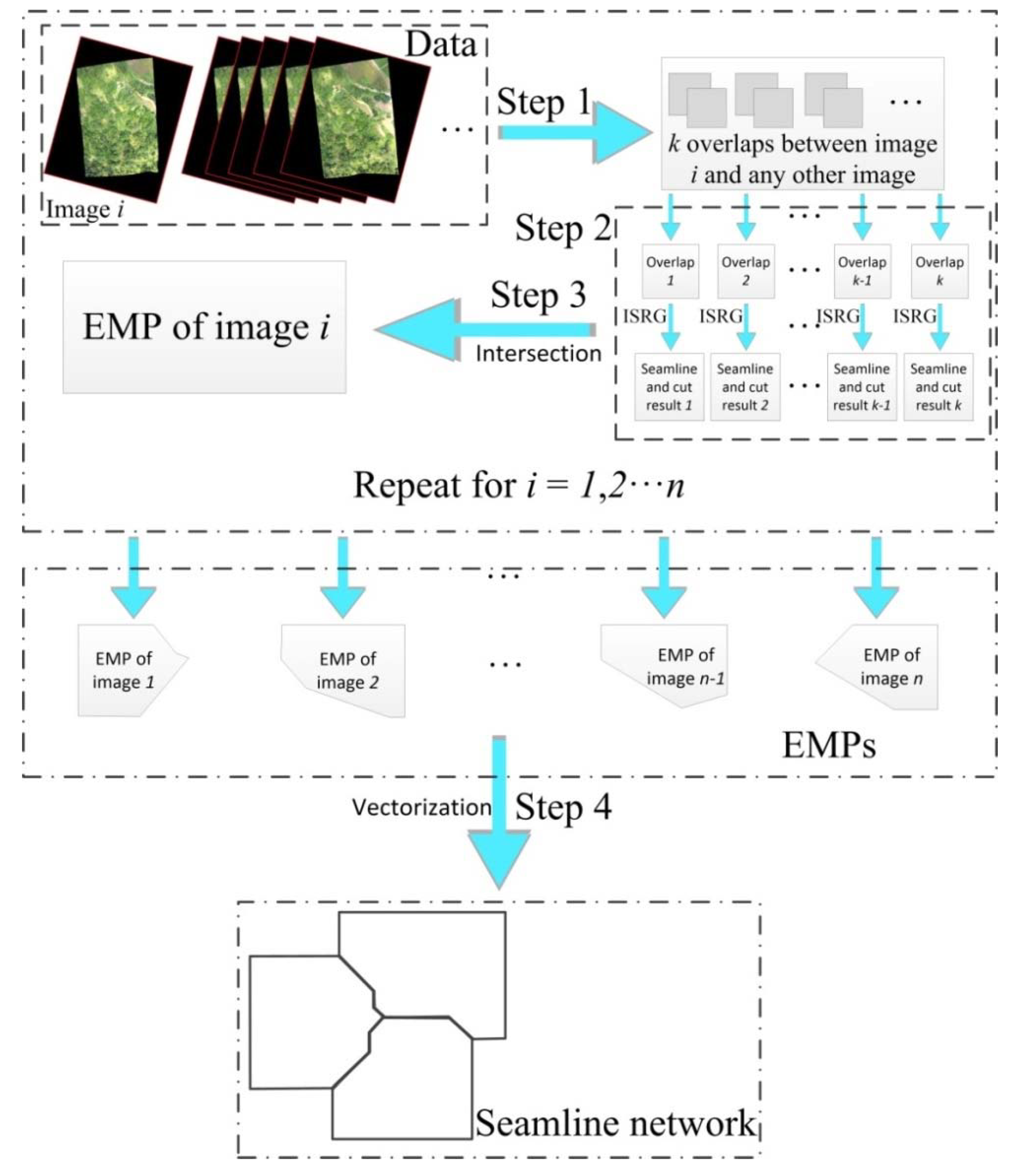
2.1. Obtaining Effective Areas and Overlap Regions between Images

After geometric rectification, each orthoimage is usually composed of the effective area and invalid area. To prevent seamlines from falling into invalid areas, which may result in unnecessary holes in the final mosaicking image, it is necessary to determine the effective area of each orthoimage, i.e., the polygon of pixels with valid pixel values. This procedure is carried out using the boundary tracking algorithm [21]. Then, supposing the effective area of image i ($1\le i\le n$) has overlaps with the effective areas of other k ($0\le k<n$) images, these k overlaps are obtained using polygon intersection. The n orthoimages are represented as I₁, I₂, …, I_n, and the indexes of images are dependent on the input order. Their effective areas are represented as P₁, P₂, …, P_n, and the k overlap regions between image i and other images are represented as O_i1, O_i2, …, O_ik.

2.2. Generation of the Seamline and the Corresponding Cut Result

For arbitrary overlap region O_is ($1\le s\le k$), i.e., the overlap region between image i and image s, the improved seeded region growing algorithm is used to determine the seamline. The boundaries of overlap region O_is are chosen as seeds. These seeds grow simultaneously until a separatrix between growing regions is generated, which is the seamline in the overlap region. Detailed steps are as follows.

Step 1: Create a template matrix for image i and s, i.e., ${\mathrm{M}}_{is}$, to record the spatial relationship of the two images. This template matrix is an image with the same size as the mosaic of image i and s. The coverage area of the template matrix can be calculated according to the obtained effective area polygons, P_i and P_s. The size of the template matrix is calculated by Equation (1) and Equation (2). Then, the template matrix can be generated, in which all initial values are set to zero.

$$Cols=\lceil \left(X_{max}-X_{min}\right)/Re{s}_x\rceil$$

(1)

$$Rows=\lceil \left(Y_{max}-Y_{min}\right)/Re{s}_y\rceil$$

(2)

where Cols and Rows represent the size of the template matrix, X_max, X_min, and Res_x represent the maximum coordinate, the minimum coordinate, and the ground resolution of the template matrix in the horizontal direction; Y_max, Y_min, and Res_y represent the maximum coordinate, the minimum coordinate, and the ground resolution of the template matrix in the vertical direction.

Step 2: Fill the template matrix ${\mathrm{M}}_{is}$ using the scan-line filling algorithm [22]. The effective area of each image is composed of the overlap region and non-overlapping region. For pixels in the effective area of image i, if a pixel falls in the non-overlapping region, the corresponding pixel in ${\mathrm{M}}_{is}$ is set to i. For pixels in the effective area of image s, if a pixel falls in the non-overlapping region, the corresponding pixel in ${\mathrm{M}}_{is}$ is set to s. Finally, for the pixels falling in the overlap region of image i and image s, the corresponding pixels in ${\mathrm{M}}_{is}$ are set to n + 1.

Step 3: Generate the seamline in the overlap region O_is using the improved seeded region growing algorithm. The seeds of the classic seeded region growing algorithm [23] are individual points. In the region growing procedure proposed in this paper, the boundary lines of the overlap region are considered the seeds to generate the bisector of the overlap region. The illustration of the improved seeded region growing algorithm is shown in Figure 2. Figure 2a shows the overlap region and the generated seamline. In Figure 2a, image i and image s are two images with overlap. Polygon ABCD is the overlap region of the two adjacent images. Point A and point C are intersected points of effective areas’ boundaries for the two adjacent images. Using the boundary tracking algorithm, the boundary of the overlap region can be obtained, which is represented as polyline ABCDA in Figure 2a. From point A to point C, there are two paths along the boundary of the overlap region: polyline ABC and polyline ADC. These two polylines are chosen as seeds. These seeds grow simultaneously until they generate a separatrix between growing regions, shown as the red line in Figure 2a. The region growing procedure is shown in Figure 2b. In Figure 2b, each small square represents a pixel in the overlap region. The dark-shadowed region is the growing region of image i, where values of corresponding pixels in ${\mathrm{M}}_{is}$ are changed to i. The light-shadowed region is the growing region of image s, where values of corresponding pixels in ${\mathrm{M}}_{is}$ are changed to s. After growing, there will be a separatrix in the overlap region, which is represented as the red region in Figure 2b. This generated separatrix is regarded as the seamline in the overlap region. Besides the seamline, the corresponding cut result for image i and image s are also generated, shown in Figure 2c. In Figure 2c, the left image is the result of cutting image i along the generated seamline, while the right one is the result of cutting image s along the generated seamline. A pseudocode is used to explain the seeded region growing procedure in the following. ABC and ADC are selected as the growing seeds, seed₁ and seed₂. S is the generated separatrix in the overlap region, and it is also regarded as the generated seamline.

1:

Seed₁ ← ABC

2:

Seed₂ ← ADC

3:

S ← Φ

4:

IfS does not generate

5:

Do seed growing using Seed₁ and Seed₂ simultaneously to generate S

6:

return S

Step 4: These steps are repeated for the k overlap regions. In this way, the cut results of all seamlines for image i are obtained.

2.3. Determination of Each Image’s EMP

When all k overlap regions of image i are processed, k seamlines and k corresponding cut results of image i are also generated. Then, the EMP of image i can be determined by intersecting the generated k cut results. The region in which each pixel has the same value, i.e., i, in all cut results is the EMP of image i. The illustration of EMP determination is shown in Figure 3. Suppose there are three images: image I₁, image I₂, and image I₃. Figure 3a shows the arrangement of the images according to geocoding. There are two overlap regions between image I₁ and the other two images: C₁ between image I₁ and image I₂ shown in Figure 3b, and C₂ between image I₁ and image I₃ shown in Figure 3c. Using the boundary tracking algorithm, the boundary of C₁ can be obtained. According to the two intersected points of the effective areas’ boundaries for image I₁ and image I₂, the boundary of C₁ can be divided into two parts, which are shown as the blue dotted line and yellow dotted line in Figure 3b. These two parts are chosen as seeds. Then, the improved seeded region growing algorithm is applied to determine the generated seamline in C₁, i.e., the red line in Figure 3b. The same processing is repeated to determine the seamline in C₂, i.e., the red line in Figure 3c. For each seamline, a cut result for image I₁ is also generated. Figure 3d shows the result of cutting image I₁ along the generated seamline in C₁, and Figure 3e shows the result of cutting image I₁ along the generated seamline in C₂. Figure 3f shows the arrangement of the two cut results of image I₁ according to geocoding. They are intersected to determine the EMP of image I₁, which is shown in Figure 3g. The above steps are repeated for image I₂ and I₃. Then, the EMPs of image I₁, image I₂, and image I₃ are determined, which are shown in Figure 3h.

2.4. Vectorization to Generate the Seamline Network

After obtaining the EMPs of all images, the vectorization processing is a necessary step to generate the seamline network. In this study, the vectorization method from [24] was adopted. The vectorization method contains four steps. First, all the possible nodes and coordinate points are extracted from the raster image. Because the extracted vector point corresponds to the position between four pixels, the size of the extraction window is 2 × 2 pixels. According to the extraction window, there are 11 cases shown in Figure 4. In Figure 4, Cases 1–5 belong to coordinate points and Cases 6–11 belong to nodes. Because these points extracted from the image are all isolated points, it is necessary to establish connection information between these points. Finally, these points are connected to generate arcs based on the connection information. By these means, the polygons and their topological relation are generated.

3. Results

The presented algorithm was implemented using the C++ language to verify its feasibility. In addition, the Geospatial Data Abstraction Library (GDAL) was used to read and write images. A desktop computer with a 64-bit Windows 7 operating system, an Intel Xeon E3 CPU at 3.0 GHz, a memory with a capacity of 16 GB, and a hard disk with a capacity of 1 TB was utilized for the experiments. Two data sets, called Data Set 1 and Data Set 2, were used in this work.

3.1. Experiment 1

In Experiment 1, a group of orthorectified images were selected as experimental data, called Data Set 1. Data Set 1 was composed of 11 orthoimages, whose ground resolutions were 0.6 m. The size of each image was approximately 2000 by 3000 pixels. There were jagged edges in the images, which led to concave polygonal overlap regions between images. The arrangement of Data Set 1 is shown in Figure 5. These orthoimages were placed according to their geocoding information, and their invalid area values are ignored. Each image contains effective areas and invalid areas. The red wireframes represent the effective area of each image. It can be seen that there are concave polygonal overlap regions, such as the blue rectangular area.

The generated seamline network overlapping the mosaic of Data Set 1 by the presented method is shown in Figure 6. The generated seamline network is represented by the cyan lines. According to the generated seamline network, it is obvious that the presented method can process concave polygonal overlap regions successfully. Two contrasting subregions of the same location, i.e., the marked blue rectangular area in Figure 5 and Figure 6, are further compared in detail in Figure 7. Figure 7a and Figure 7b show details of the blue rectangular area marked in Figure 5 and Figure 6, respectively. As shown in Figure 7a, there are several concave polygonal overlap regions. Figure 7b shows details of the generated seamline network in the same location as Figure 7a. It is obvious that the presented method can process concave polygonal overlap regions successfully.

3.2. Experiment 2

In Experiment 2, 21 orthoimages were selected as the experimental data, i.e., Data Set 2. Data Set 2 was a group of UAV images. The size of each image is approximately 1700 by 2100 pixels, and the ground resolution is 0.1 m. The arrangement of Data Set 2 is shown in Figure 8. These orthoimages were placed according to their geocoding information, and their invalid area values were ignored. Similarly, the red wireframes represent the effective area of each image. Figure 9 is the generated seamline network overlapping the mosaic of Data Set 2 by the presented method. The generated seamline network is represented by the cyan lines. It can be seen that the method proposed in this paper processed Data Set 2 precisely.

3.3. Comparative Experiments

To analyze and evaluate the advantages and disadvantages of the presented method, comparative experiments were designed. Pan et al.’s (2014) method [15], Wan et al.’s (2013) method [25], and the method in ERDAS IMAGE 2018 were chosen for the comparative experiments. Because ERDAS IMAGE 2018 cannot process the map projection of Data Set 1, the method in ERDAS IMAGE 2018 was only used to process Data Set 2.

The generated seamline network overlapping the mosaic of Data Set 1 by Pan et al.’s (2014) method is shown in Figure 10a, while Figure 10b shows the generated seamline network overlapping the mosaic of Data Set 1 by Wan et al.’s (2013) method. In Figure 10, the generated seamline network is represented by the cyan lines. Detailed comparisons of Pan et al.’s (2014) method, Wan et al.’s (2013) method, and the presented method are shown in Figure 11. Figure 11a is the yellow rectangular area marked in Figure 5, i.e., details of the original orthoimage. Figure 11b is the yellow rectangular area marked in Figure 10a, i.e., details of Pan et al.’s (2014) method. Figure 11c is the yellow rectangular area marked in Figure 10b, i.e., details of Wan et al.’s (2013) method. Figure 11d is the yellow rectangular area marked in Figure 6, i.e., details of the presented method. It can be seen from the comparison results that Wan et al.’s (2013) method and the presented method can obtain a more accurate seamline network than Pan et al.’s (2014) method.

Figure 12 and Figure 13 compare Pan et al.’s (2014) method, Wan et al.’s (2013) method, and the presented method applied to Data Set 2. Figure 12a shows the processing results of Pan et al.’s (2014) method, while Figure 12b shows the processing results of Wan et al.’s (2013) method. It is obvious that there are some errors in the processing result of Pan et al.’s (2014) method, for example, the red oval area and blue rectangular area. The red oval area is a boundary error, while the blue rectangular area is a hole in the mosaic. The reason is that Pan et al.’s (2014) method uses convex hulls of the actual effective areas of the images as their approximate effective areas to avoid processing concave polygonal overlaps. The presented method and Wan et al.’s (2013) method obtain satisfactory seamline networks. This can be seen more clearly in the detailed comparison in Figure 13. Figure 13a is the blue rectangular area marked in Figure 8, i.e., details of the original orthoimages. Figure 13b is the blue rectangular area marked in Figure 12a, i.e., details of Pan et al.’s (2014) method. Figure 13c is the blue rectangular area marked in Figure 12b, i.e., details of Wan et al.’s (2013) method. Figure 13d is the blue rectangular area marked in Figure 9, i.e., details of the presented method.

The processing results of the method in ERDAS IMAGE 2018 is shown in Figure 14a, in which the blue lines represent the generated seamline network. It is clear that there are many small chips in the generated seamline network, such as the black rectangular areas marked in Figure 14a. These small chips may introduce difficulties for seamline optimization because there are not enough areas to determine the best seamline. In order to show this clearly, the black rectangular areas marked in Figure 14a are enlarged in Figure 14b and Figure 14c. In addition, when the order of compositing is changed, a different seamline network is generated by the method in ERDAS IMAGE 2018. A different seamline network of Data Set 2 generated by the method in ERDAS IMAGE 2018 is shown in Figure 15, which indicates that the method in ERDAS IMAGE 2018 is dependent on the composite sequence of images.

To evaluate these results quantitatively, the overall accuracy (OA) and kappa coefficient (k) [26] were chosen to represent the accuracy of the generated seamline network. In addition, the error rate (E) and miss rate (M) of the effective areas were also used to evaluate the accuracy of the generated seamline network. In this paper, the analysis of the generated seamline network is similar to the analysis of binary classification in remote sensing. The original image is the ground truth, and the mosaic image formed based on the generated seamline network is the result of classification. There are two categories in the mosaic image: (1) the pixels in the effective areas of the original images, i.e., correct region, and (2) the pixels in the invalid areas of the original images, i.e., error region. Then, based on a confusion matrix [27], the overall accuracy, the kappa coefficient, the error rate, and the miss rate of the effective areas are calculated using Equation (3), Equation (4), Equation (5), and Equation (6).

$$OA=\frac{{\sum }_{i=1}^2{X}_{ii}}{N}$$

(3)

$$k=\frac{N\times {\sum }_{i=1}^2{X}_{ii}-{\sum }_{i=1}^2\left(T_i\times S_i\right)}{N^2-{\sum }_{i=1}^2\left(T_i\times S_i\right)}$$

(4)

$$E=\frac{X_{21}}{S_1}$$

(5)

$$M=\frac{X_{12}}{S_1}$$

(6)

where OA is the overall accuracy, k is the kappa coefficient, E and M are the error rate and the miss rate of the effective areas. The more accurate the generated seamline network, the larger the values of the overall accuracy and the kappa coefficient, and the smaller the error rate and miss rate of the effective areas. i represents the category index, which is set to 1 or 2. X_ii represents the number of pixels belonging to the same category. N is the number of all pixels, S_i represents the number of one category’s pixels for the original image, and T_i represents the number of one category’s pixels for the mosaic image.

As demonstrated in Figure 16, polygon ABCD is a mosaic image formed based on the generated seamline network, the white area is the effective area in the original image, and the gray area is the invalid area in the original image. If polygon abcd is the mosaic area formed by the generated seamline network, polygon dfe and polygon afg are the error regions. Polygon dfe is in invalid areas in the original image, but it is included in the mosaic area. Polygon afg is in the effective areas in the original image but excluded from the mosaic area. Therefore, a confusion matrix can be obtained, which is demonstrated in

Table 1. Demonstration of the confusion matrix.

	In the Mosaic Area	Outside of the Mosaic Area	Total
In effective areas in original images	X11	X12	S1
In invalid areas in original images	X21	X22	S2
Total	T1	T2	N

. In Table 1, pixels in the original images are divided into pixels in the effective areas and pixels in the invalid areas. For the final mosaic, pixels are divided into pixels in the mosaic area and pixels outside of the mosaic area. X₁₁ represents the number of pixels which are in the effective areas of the original images and are also in the mosaic area, i.e., the number of pixels in the polygon abcdef in Figure 14; X₁₂ represents the number of pixels which are in the effective areas of the original images and outside of the mosaic area, i.e., the number of pixels in the polygon afg in Figure 14; X₂₁ represents the number of pixels which are in invalid areas of the original images but in the mosaic area, i.e., the number of pixels in the polygon dfe in Figure 14; X₂₂ represents the number of pixels which are in invalid areas of the original images and outside of the mosaic area, i.e., the number of pixels in the grey area but exclude polygon dfe in Figure 14. S₁ represents the number of pixels in the effective areas in the original images; S₂ represents the number of pixels in invalid areas in the original images; T₁ represents the number of pixels in the mosaic area; T₂ represents the number of pixels outside of the mosaic area. N is the number of all pixels. Then, the overall accuracy, the kappa coefficient, the error rate, and the miss rate of the effective areas can be calculated by Equation (3), Equation (4), Equation (5), and Equation (6).

Table 2. Quantitative comparisons.

Data	Method	T/ms	k	OA	E	M
Data Set 1	This paper’s method	17,347	1.0	1.0	0.0	0.0
	Pan et al.’s (2014) method	343	0.9801	0.9901	0.0001	0.0204
	Wan et al.’s (2013) method	10,624 + Δ 1	1.0	1.0	0.0	0.0
Data Set 2	This paper’s method	49,187	1.0	1.0	0.0	0.0
	Pan et al.’s (2014) method	725	0.9838	0.9919	0.0130	0.0026
	Wan et al.’s (2013) method	13,885 + Δ 1	1.0	1.0	0.0	0.0
	The method in ERDAS	55,750	1.0	1.0	0.0	0.0

¹: the time consumed to input the strip information manually.

shows the quantitative comparison of these methods. Both the time consumed and accuracy of the generated seamline network are taken into account. With respect to the time consumed, it is clear that Pan et al.’s (2014) method can generate the seamline network much more efficiently than the other three methods, as shown in Table 2. For Data Set 1 and Data Set 2, Pan et al.’s (2014) method only took 343 ms and 725 ms, respectively, while the presented method took 17,347 ms and 49,187 ms, respectively. Wan et al.’s (2013) method took much more time because there was no strip information for Data Set 1 and Data Set 2. The manual input of strip information took a few minutes to more than 10 min. In Table 2, the time used for manual input of strip information is represented by Δ, and it depends on the number of images and the complexity of their arrangement. When the strip information is ambiguous, different people may define different strip information, and different seamline networks will be generated. If the strip information is not regular, the effect of the final mosaic may also be influenced. If not considering the time spent on manually inputting strip information, Wan et al.’s (2013) method took 10,624 ms and 13,885 ms for Data Set 1 and Data Set 2, respectively, when obtaining the image boundaries and generating the seamline network. The method in ERDAS IMAGE 2018 took 55,750 ms for Data Set 2. With respect to accuracy, Wan et al.’s (2013) method, the method in ERDAS IMAGE 2018, and the presented method obtained better performances than Pan et al.’s (2014) method. For Data Set 1 and Data Set 2, Wan et al.’s (2013) method and the presented method both obtained 1.0 for overall accuracy and kappa coefficient, and 0.0 for the error rate and the miss rate of the effective areas. For Data Set 2, the method in ERDAS IMAGE 2018 obtained the same accuracy as Wan et al.’s (2013) method and the presented method. Pan et al.’s (2014) method obtained less accurate results. For Data Set 1, its kappa coefficient is 0.9801, its overall accuracy is 0.9901, and its error rate and miss rate of effective areas are 0.0001 and 0.0204, respectively. For Data Set 2, its kappa coefficient is 0.9838, its overall accuracy is 0.9919, and its error rate and miss rate of effective areas are 0.0130 and 0.0026, respectively. Therefore, it is obvious that the presented method is better than the other three methods, and it has the advantages of high accuracy and automation without other input information. In addition, the seamline network generated by the proposed method is global-based and is independent of the sequence of the image compositing. Of course, compared with the AVDO-based method, it also has the disadvantage of greater time spent.

4. Discussion

4.1. The Relationship between Processing Time, Accuracy, and the Down-Sampling Rate

The method in this paper is based on raster data, which is time-consuming. In practice, efficiency has to be taken into consideration. To address the problem, in this study, down-sampling was applied to reduce images’ ground resolution and improve the timing of the process. Figure 17 is the statistical result of processing times when applying different down-sampling rates to Data Set 1. In Figure 17, the horizontal axis represents down-sampling rates, while the vertical axis represents processing time, and the unit of processing time is a millisecond.

From this line chart, it is obvious that improving the down-sampling rate can significantly improve the efficiency of the presented method. When there is no down-sampling, the processing time for this method is 17,347 ms, while, when the down-sampling rate is 5, the processing time is only 1778 ms. This is a significant improvement in efficiency. The larger the down-sampling rate, the shorter the processing time.

However, accuracy has to be considered when increasing the down-sampling rate. Figure 18 shows the changing trend in accuracy while increasing the down-sampling rates and also reveals the relationship between accuracy and down-sampling rate. In Figure 18, the horizontal axis represents the down-sampling rates, while the vertical axis represents accuracy. The accuracy is represented by the overall accuracy (OA) and kappa coefficient (k). It is obvious that when applying the larger down-sampling rate, a lower accurate seamline network is obtained. When there is no down-sampling, the overall accuracy and the kappa coefficient are all 1.0. When the down-sampling rate is 5, the overall accuracy and the kappa coefficient are 0.9855 and 0.9712, respectively.

In a word, the relationship between the processing time and accuracy needs to be taken into consideration, and there must be some compromise between the time cost and accuracy, in practice. Down-sampling rates need to be chosen carefully according to the actual requirement for accuracy or processing time.

4.2. The Data Type of Template Matrix

In this study, the template matrix was an essential intermediate to obtain the EMP of each image. The template matrix data type can be chosen properly according to the number of images. If there are n images, and the template matrix data type is m bits, then Equation (7) needs to be met.

$$n+1\le 2^m-1$$

(7)

If the template matrix storage size is much bigger than its actual demands, the processing efficiency is reduced. Conversely, if the template matrix storage size is smaller than its actual demands, there will be mistakes during processing. Thus, it is necessary to choose a proper template matrix data type for mosaicking and improving the efficiency.

5. Conclusions

In this paper, we present a seamline network generation method based on improved seeded region growing, which can be regarded as an improvement of the AVDO-based method [13,15]. In the presented method, two boundaries of an overlap region are set as seeds of the improved seeded region growing algorithm, which is designed to obtain the bisector of the overlap region. In this way, the method presented in this paper can process any kind of overlap region and obtain highly accurate seamline network and mosaicking results. Experimental results were satisfactory, and our method processed the concave polygonal overlap regions successfully. Compared with the AVDO-based method [13,15], the method proposed in this paper can process concave polygonal overlap regions successfully and obtain more accurate seamline networks, but the processing time is much longer. With respect to Wan et al.’s (2013) method [25], the presented method has an added advantage of not requiring any other input information. In addition, the presented method is independent of the sequence of the image composite.

Down-sampling was used to improve the efficiency of the proposed method. Experimental results indicate that the processing time can be reduced by down-sampling. However, as the down-sampling rate increased, the accuracy of the generated seamline network decreased. Therefore, studies to improve the efficiency of the presented method while ensuring the high accuracy of the generated seamline network are necessary. Considering that the seamline network generated by the proposed method is global-based and independent of the sequence of the image composite, parallel technology will also be implemented to improve efficiency in the future.

References

1. Chon, J.; Kim, H.; Lin, C.S. Seam-line determination for image mosaicking: A technique minimizing the maximum local mismatch and the global cost. ISPRS J. Photogramm. Remote Sens. 2010, 65, 86–92. [Google Scholar] [CrossRef]
2. Afek, Y.; Brand, A. Mosaicking of Orthorctified Aerial Image. Photogramm. Eng. Remote Sens. 1998, 64, 115–125. [Google Scholar]
3. Peleg, S.; Rousso, B.; Ravacha, A.; Zomet, A. Mosaicing on Adaptive Manifolds. IEEE Trans. Pattern Anal. Mach. Intell. 2000, 22, 1144–1154. [Google Scholar] [CrossRef]
4. Hu, F.; Li, T.; Geng, Z. Constraints-based graph embedding optimal surveillance-video mosaicking. In Proceedings of the First Asian Conference on Pattern Recognition, Beijing, China, 28 November 2011; pp. 311–315. [Google Scholar]
5. Brown, M.; Lowe, D.G. Automatic Panoramic Image Stitching using Invariant Features. Int. J. Comput. Vis. 2007, 74, 59–73. [Google Scholar] [CrossRef]
6. Xandri, R.; Pérez, F.; Palà, V.; Arbiol, R. Automatic generation of seamless mosaics over extensive areas from high resolution imagery. In Proceedings of the 9th World Multi-Conference on Systemics, Cybernetics and Informatics, Informatics, Orlando, FL, USA, 13 July 2005; pp. 1–6. [Google Scholar]
7. Yang, Y.; Gao, Y.; Li, H.; Han, Y. An Algorithm for Remote Sensing Image Mosaic Based on Valid Area. In Proceedings of the IEEE International Symposium on Image and Data Fusion, Tengchong, China, 9–11 August 2011; pp. 1–4. [Google Scholar]
8. Wang, D.; Wan, Y.; Xiao, J.; Lai, X.; Huang, W.; Xu, J. Aerial Image Mosaicking with the Aid of Vector Roads. Photogramm. Eng. Remote Sens. 2012, 78, 1141–1150. [Google Scholar] [CrossRef]
9. Chen, Q.; Sun, M.; Hu, X.; Zhang, Z. Automatic Seamline Network Generation for Urban Orthophoto Mosaicking with the Use of a Digital Surface Model. Remote Sens. 2014, 6, 12334–12359. [Google Scholar] [CrossRef] [Green Version]
10. Pang, S.; Sun, M.; Hu, X.; Zhang, Z. SGM-based seamline determination for urban orthophoto mosaicking. ISPRS J. Photogramm. Remote Sens. 2016, 112, 1–12. [Google Scholar] [CrossRef]
11. Hsu, S.; Kumar, R. Automated mosaics via topology inference. Comput. Graph. Appl. IEEE 2002, 22, 44–54. [Google Scholar] [CrossRef]
12. Ma, H.C.; Sun, J. Intelligent optimization of seam-line finding for orthophoto mosaicking with LiDAR point clouds. J. Zhejiang Univ. Sci. C 2011, 12, 417–429. [Google Scholar] [CrossRef]
13. Pan, J.; Wang, M.; Li, D.; Li, J. Automatic Generation of Seamline Network Using Area Voronoi Diagrams with Overlap. IEEE Trans. Geosci. Remote Sens. 2009, 47, 1737–1744. [Google Scholar] [CrossRef]
14. Mills, S.; Mcleod, P. Global seamline networks for orthomosaic generation via local search. ISPRS J. Photogramm. Remote Sens. 2013, 75, 101–111. [Google Scholar] [CrossRef]
15. Pan, J.; Wang, M.; Ma, D.; Zhou, Q.; Li, J. Seamline Network Refinement Based on Area Voronoi Diagrams with Overlap. IEEE Trans. Geosci. Remote Sens. 2014, 52, 1658–1666. [Google Scholar] [CrossRef]
16. Fernandez, E.; Garfinkel, R.; Arbiol, R. Mosaicking of Aerial Photographic Maps via Seams Defined by Bottleneck Shortest Paths. Oper. Res. 1998, 46, 293–304. [Google Scholar] [CrossRef]
17. Kerschner, M. Seamline detection in colour orthoimage mosaicking by use of twin snakes. ISPRS J. Photogramm. Remote Sens. 2001, 56, 53–64. [Google Scholar] [CrossRef]
18. Pan, J.; Wang, M.; Li, J.; Yuan, S.; Hu, F. Region change rate-driven seamline determination method. ISPRS J. Photogramm. Remote Sens. 2015, 105, 141–154. [Google Scholar] [CrossRef]
19. Li, L.; Yao, J.; Liu, Y.; Yuan, W.; Shi, S.Z.; Yuan, S.G. Optimal Seamline Detection for Orthoimage Mosaicking by Combining Deep Convolutional Neural Network and Graph Cuts. Remote Sens. 2017, 9, 701. [Google Scholar] [CrossRef]
20. Dong, Q.; Liu, J. Seamline Determination Based on PKGC Segmentation for Remote Sensing Image Mosaicking. Sensors 2017, 17, 1721. [Google Scholar] [CrossRef] [PubMed]
21. Moradi, J.Y.; Pappas, M. A Boundary Tracking Optimization Algorithm for Constrained Nonlinear Problems. J. Mech. Des. 1978, 100, 292–296. [Google Scholar] [CrossRef]
22. Pan, J.; Wang, M.; Li, Q. Fast mosaic algorithm based on scanning line filling. Sci. Surv. Mapp. 2006, 31, 8–9. [Google Scholar]
23. Adams, R.; Bischof, L. Seeded region growing. IEEE Trans. Pattern Anal. Mach. Intell. 1994, 16, 641–647. [Google Scholar] [CrossRef]
24. Chen, R.X.; Zhao, Z.M.; Pan, J. A Fast Method of Vectorization for RS Classified Raster Map. J. Remote Sens. 2006, 10, 326–331. [Google Scholar]
25. Wan, Y.; Wang, D.; Xiao, J.; Lai, X.; Xu, J. Automatic determination of seamlines for aerial image mosaicking based on vector roads alone. ISPRS J. Photogramm. Remote Sens. 2013, 76, 1–10. [Google Scholar] [CrossRef]
26. Du, P.; Tan, K.; Xing, X. A novel binary tree support vector machine for hyperspectral remote sensing image classification. Opt. Commun. 2012, 285, 3054–3060. [Google Scholar] [CrossRef]
27. Stehman, S.V. Selecting and interpreting measures of thematic classification accuracy. Remote Sens. Environ. 1997, 62, 77–89. [Google Scholar] [CrossRef]
Figure 1. The flowchart of the improved seeded region growing-based seamline network generation method. ISGR: improved seeded region growing algorithm; EMP: effective mosaic polygon.
Remotesensing 10 01065 g001
Figure 2. The illustration of the improved seeded region growing algorithm: (a) the illustration of the overlap region and the generated seamline; (b) the procedure of improved seeded region growing; (c) results of cutting image i and image s along the generated seamline.
Remotesensing 10 01065 g002
Figure 3. The illustration of EMP determination: (a) the arrangement of images according geocoding; (b) the generated seamline of C1; (c) the generated seamline of C2; (d) the result of cutting image I1 by C1; (e) the result of cutting image I1 by C2; (f) the arrangement of the two cut results for image I1; (g) the EMP of image I1; (h) EMPs of image I1, image I2, and image I3.
Remotesensing 10 01065 g003
Figure 4. Eleven cases of points [24].
Remotesensing 10 01065 g004
Figure 5. Data Set 1.
Remotesensing 10 01065 g005
Figure 6. The generated seamline network overlapping the mosaic of Data Set 1 by the presented method.
Remotesensing 10 01065 g006
Figure 7. Details of (a) the blue rectangular area marked in Figure 5; (b) the blue rectangular area marked in Figure 6.
Remotesensing 10 01065 g007
Figure 8. Data Set 2.
Remotesensing 10 01065 g008
Figure 9. The generated seamline network overlapping the mosaic of Data Set 2 by the presented method.
Remotesensing 10 01065 g009
Figure 10. Results: (a) the generated seamline network overlapping the mosaic of Data Set 1 by Pan et al.’s (2014) method; (b) the generated seamline network overlapping the mosaic of Data Set 1 by Wan et al.’s (2013) method.
Remotesensing 10 01065 g010
Figure 11. Details of (a) the yellow rectangular area marked in Figure 5; (b) the yellow rectangular area marked in Figure 10a; (c) the yellow rectangular area marked in Figure 10b; (d) the yellow rectangular area marked in Figure 6.
Remotesensing 10 01065 g011
Figure 12. Results: (a) the generated seamline network overlapping the mosaic of Data Set 2 by Pan et al.’s (2014) method; (b) the generated seamline network overlapping the mosaic of Data Set 2 by Wan et al.’s (2013) method.
Remotesensing 10 01065 g012aRemotesensing 10 01065 g012b
Figure 13. Details of (a) the blue rectangular area marked in Figure 8; (b) the blue rectangular area marked in Figure 12a; (c) the blue rectangular area marked in Figure 12b; (d) the blue rectangular area marked in Figure 9.
Remotesensing 10 01065 g013
Figure 14. (a) The generated seamline network by the method in ERDAS IMAGE 2018; (b) the black rectangular area a marked in Figure 14a; (c) the black rectangular area b marked in Figure 14a.
Remotesensing 10 01065 g014
Figure 15. A different seamline network generated by the method in ERDAS IMAGE 2018 for a different image composite sequence.
Remotesensing 10 01065 g015
Figure 16. Demonstration of two categories.
Remotesensing 10 01065 g016
Figure 17. Relationship between processing time and down-sampling rate.
Remotesensing 10 01065 g017
Figure 18. Relationship between the accuracy and the down-sampling rate.
Remotesensing 10 01065 g018